Modeling of Fire Contagion in Farms Insurance

1. Introduction

A single fire can sometimes generate large losses because it can spread to buildings near the origin. Naturally, such a risk is of interest to actuaries. In this paper, we propose a new ratemaking model in which fire contagion is a main concern. The model is applied to farm insurance, where a single farm may have several types of structures: dwellings, barns, granaries, silos, and so on. As these structures can be close to each other, all structures of a farm can be touched by a single fire. Indeed, as we will see in the numerical illustration shown in this paper, summary statistics show that a fire beginning in one structure can often spread to other structures of the same farm.

To estimate the risk of fire damages, the characteristics of each farm and structures of that farm should be used for modeling. However, given the limited literature and the limited data on the subject at the present time, we will instead focus on studying fire contagion mainly as a function of the distances between structures. Indeed, a fire is more likely to propagate when a farm’s structures are located near each other. Using satellite images of 39 different farms as well as policy and claim information from the years 2014–2019, we propose a model of fire contagion having the objective of pricing each structure of a given farm. We believe that the proposed approach is an interesting first step in developing a more general approach for the modeling of fire propagation in farm insurance, or even in commercial or home insurance.

1.1. Literature review

To our knowledge, there does not seem to be a body of literature relating to fire propagation with an application to farm insurance, home insurance, or commercial insurance. Carlsson (1999) studies prevention measures to counter the spread of fire between different buildings. The author mentions that the most important factors in fire contagion are fire temperature and fire distance. The author concludes that the dimensions of the buildings, the size of the windows, as well as the types of materials and contents have a great influence on the temperature reached by the fire and thus the possibility of the fire spreading. Pesic et al. (2017) relate simulations used to measure the impact of distance between residential buildings. The authors conclude that the risk of propagation between buildings is negligible for distance of 4.5 meters or greater, but larger buildings are not considered in the study.

Apart from contagion, however, it seems that the study of fire risk rate has been studied for many years. Indeed, as mentioned by Johansen (1979), who lists Italian mathematicians from the mid-20th century, it has been known for a long time that “the fire risk rate increases with the size of the insured object in a similar way as the death rate increases with the age.” But this analysis of fire seems to rather focus on the damages from direct fire and not from contagion. Researches on the modeling of wildfires and its impact on the insurance market have become more popular in recent years (Rodriguez-Baca, Raulier, and Leduc 2016), but the fire contagion phenomenon of wildfires has little to do with fires that can spread to multiple structures of the same farm. Also, obviously, basic physics research on fire phenomena has been done (see Drysdale 2011 for an introduction), but the information found in that kind of research is not useful for actuaries who are looking for methods to compute annual premiums or techniques for risk management.

Research in actuarial science with applications to farm insurance has not been popular either; it sometimes focuses on crop insurance (Just, Calvin, and Quiggin 1999; Pigeon, Frahan, and Denuit 2012) rather than farm structures and their contents. Statistical methods developed by actuaries are mainly based on automobile insurance (see Denuit et al. 2007 or Frees, Derrig, and Meyers 2014 for an overview). But those pricing and risk management techniques developed in the actuarial literature can obviously be generalized to other insurance products. Indeed, whether actuaries work in auto, home, or farm insurance, the theoretical basis for modeling claim frequency and claim severity appears to remain the same. The number of claims remains a discrete random variable, where risk characteristics can be included in the parameters of the model, and the claim severity distribution is likely skewed. However, as we will see in this paper, some characteristics of farm insurance require other modeling approaches to properly understand risk.

1.2. Modeling approach

The modeling of fire contagion leads to the consideration of many elements: probability of fire, probability of contagion, and severity of the damages. First, this general modeling approach of total incurred loss for a given farm, denoted $S$, will simply be based on individually modeling each structure $j=1, \ldots, J$ of that farm. In other words, the total incurred loss arising from a farm consists of the sum of the amount of losses of each of its structures:

$$\begin{aligned} S = \sum_{j=1}^J S^{(j)} \end{aligned}$$

where $S^{(j)}$ is the total claim cost of structure $j$, for $j= 1, \ldots, J$. We then have to use compound sum, that we can generalize depending on the origin of the fire:

$$\begin{aligned} S^{(j)} &= \sum_{i=1}^{N} X_i^{(j)} = \sum_{i=1}^{N_1} X_{i,1}^{(j)} + \sum_{i=1}^{N_2} X_{i,2}^{(j)} \\ &\quad + \ldots + \sum_{i=1}^{N_J} X_{i,J}^{(j)}\\ &= \sum_{k=1}^{J} \sum_{i=1}^{N_k} X_{i,k}^{(j)} \end{aligned}$$

where $N$ is the total number of fires on the farm, and $N_k, k=1, \ldots, J$ is the number of fires that originate in structure $j$, with $N = \sum_{k=1}^J N_k$. The severity of fire $i$, that originates from structure $k$, which touches structure $j$, is denoted by $X_{i,k}^{(j)}$. We suppose that all $X_{i,k}^{(j)}, i=1, \ldots, N_k$, for $k=1,\ldots, J$, are i.i.d. and independent from $N$ and all $N_k, k=1, \ldots, J$. For all such sums, we also suppose that their value is zero when $N$ or $N_k, k=1, \ldots, J$ is zero.

We can express the incurred loss for each structure $S^{(j)}$ as a function of the structure of origin. Moreover, instead of directly modeling total severity $X$, we can suppose that the total loss arising from a fire can be split into two components as $X = I \times Y$, where $I$ is a binary variable that takes the value 1 if the fire has touched the structure and 0 otherwise, and $Y$ is the severity of loss when the structure has caught fire. Appropriate indices will be affixed to $I$ and $Y$ as needed.

For example, for a specific structure $a$, we have:

$$\begin{aligned} S^{(a)} &= \sum_{i=1}^{N_a} X_{a,i}^{(a)} + \sum_{k=1, k\ne a}^J \sum_{i=1}^{N_k} X_{k, i}^{(a)} \\ &= \sum_{i=1}^{N_a} I_{a,i}^{(a)} Y_{a,i}^{(a)} + \sum_{k=1, k\ne a}^J \sum_{i=1}^{N_k} I_{k, i}^{(a)} Y_{k, i}^{(a)} \end{aligned}$$

where the first term of the above equation accounts for direct fires,^[1] and the second term accounts for damages due to fire propagation. We can compute the pure premium attributed to $a$ as the expected value of $S^{(a)}$. It can indeed be shown that:

$$\begin{aligned} E[S^{(a)}] &= E[N_a] E[X^{(a)}_{a}] \\ &\quad + \sum_{k=1, k\ne a}^J E[N_k] E[X^{(a)}_{k}] \nonumber \\ &= E[N_a] E[I^{(a)}_{a}] E[Y^{(a)}_{a}] \\ &\quad + \sum_{k=1, k\ne a}^J E[N_k] E[I^{(a)}_{k}] E[Y^{(a)}_{k}]. \end{aligned}\tag{1}$$

Note that only the second term is related to fire propagation.

1.3. Overview

As we just saw, a reasonable model of fire claims on a farm involves many random variables. In this paper, we will focus on the modeling of the contagion indicator $I$, which is covered in more detail in Section 2. The fire claim frequency, denoted by the random variable $N$, and the claim severity of each fire, denoted by $Y$, will be discussed mainly in the empirical example in Section 3. Also in Section 3, we will apply the proposed model to a portfolio of 39 farms. To estimate the parameters of the contagion component of the model, the portfolio of farm fires has been examined in detail with regard to the origin of fire and the structures affected. Distances between each insured structure have also been computed using satellite imagery. Section 4 offers a discussion on potential improvements of the model, while the last section of the paper concludes.

2. Contagion processes

2.1. General approach

A difficult task of the modeling is to find a way to evaluate (1), in other words the premium due to fire propagation. We first explain how to model $I$ before moving on to an example that will more formally define the notation in place.

Let us first define a contagion process. Suppose we wish to model the total amount of claims for structure $a$ while the origin of fire is structure $b$. Depending on the layout of the structures on the farm and the distances between those structures, there are many ways a fire starting in structure $b$ can spread to structure $a$:

1. Level 1 contagion, where the fire spread directly from structure $b$ to structure $a$

2. Level 2 contagion, where the fire spread first to another structure, and from that structure spread to structure $a$

3. Any other levels of contagions, where, more generally, for a farm with $J$ structures, there are potentially up to $J - 1$ levels of contagion, and each successive level of contagion has longer and longer paths from structure $b$ to structure $a$

We note by $P(x,y) = \frac{x!}{(x-y)!}$ the number of permutations, taking $x$ items among $y$. For a farm with $J$ structures, the number of paths $np_{\psi}$ depends on the level of contagion $\psi$ starting from structure $b$ and touching structure $a$ and will be equal to:

• Level 1: $np_1 = P(J-2,0) = 1$ path

• Level 2: $np_2 = P(J-2,1) = (J-2)$ paths

• Level 3: $np_3 = P(J-2,2) = (J-2)(J-3)$ paths

• $\ldots$

• Level $J-1$: $np_{J-1} = P(J-2,J-2) = (J-2)!$ paths.

We consider each potential path of a fire as a contagion process and assume that, of all contagion processes, at most one fire contagion is realized. Mathematically, we can see this situation as being a competition between all contagion processes to determine which one will be the cause of the fire reaching structure $a$.

We will model each contagion process by exponential random variables noted $\epsilon (\lambda)$, where the parameter $\lambda$ of the exponential distribution depends on the distance between structures $b$ and $a$ that is defined for the path of the given process. We will assume that the occurrence of fire contagion, denoted by the random variable $I$, will be a function of this $\epsilon$ process. More precisely, a structure will catch fire when $\epsilon$ is less than a certain threshold $\phi$ (arbitrarily set to 1). We thus have the probability of a specific type of contagion expressed as:

$$\begin{aligned} \Pr(I = 1) &= \Pr(\epsilon(\lambda) \le \phi = 1) \\ &= 1 - \exp(-\lambda) \end{aligned}\tag{2}$$

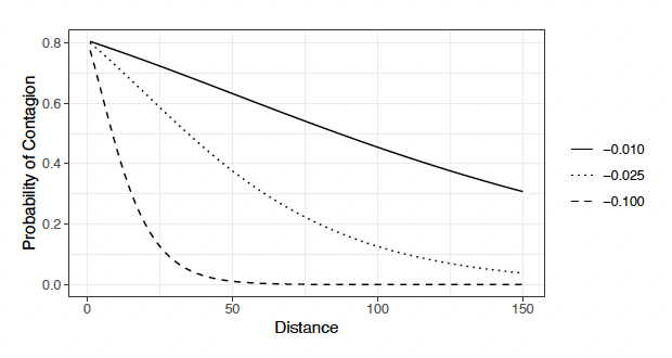
where the parameter $\lambda$ can be modeled in various ways. For example, for a level 1 contagion, we could use

$$\begin{aligned} \lambda = \exp(\beta_0 + \beta_1 d) \end{aligned}$$

where $d$ is the minimum distance between the two structures. Figure 1 illustrates the probability of contagion depending on the distance $d$, for various values of $\beta_1$. As expected, the probability of direct contagion decreases as the distance between structures increases.

Figure 1.Probability of contagion (level 1) as a function the distance between structures

More generally, for a contagion process of level $m$, we can generalize the level 1 case as:

$$\begin{aligned} \lambda &= \exp(\beta_0 + \beta_1 d_1 + \beta_2 d_2 + ... + \beta_m d_m ) \nonumber \\ &= \exp(\beta_0 + \sum_{i=1}^m \beta_i d_i) \end{aligned}\tag{3}$$

where $\beta_i, i=0, \ldots, m$ are parameters to be estimated, and $d_i, i=1, \ldots, m$ are the minimum distances between the structures present along the given path.

The overall process which summarizes all contagions is the result of competition between all contagion processes. Therefore, the prevailing contagion process can be seen as the minimum value of all $\epsilon$ processes involved. As all $\epsilon$ are exponential random variables, it can be shown that the minimum value of all $\epsilon$ will also be an exponential variable with parameter equal to the sum of all $\lambda$ parameters of contagion processes of different levels.

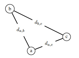
2.2. Example: Farm consisting of three structures

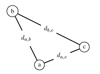
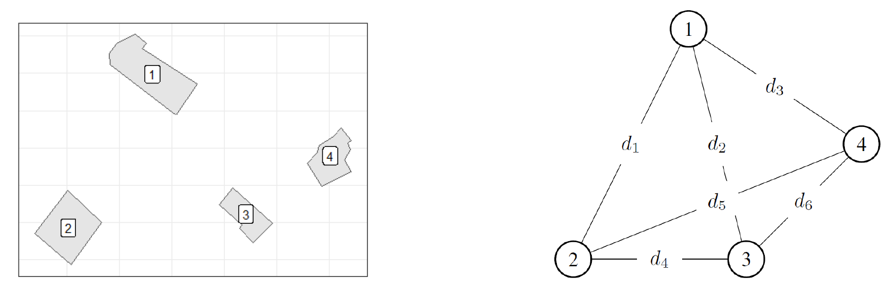
As an illustration, let us consider a farm with three structures, illustrated by Figure 2, where corresponding distances between the structures are written on each corresponding segment. Remember that, as the purpose of ratemaking is to compute the overall premium for that farm, it will be obtained by adding the premiums for each structure. For this example, we will suppose that we need to compute the premium for structure $a$.

Figure 2.Farm with 3 structures

2.2.1 Impact of fire contagion

As we want to focus on fire contagion, we first ignore the situation where a fire begins directly in structure $a$, because a fire in structure $a$ would not be due to contagion.^[2] Because we have two other structures to consider for the contagion modeling, we have to separate the approach into two components according to the origin of the fire, namely from structure $b$ or from structure $c$.

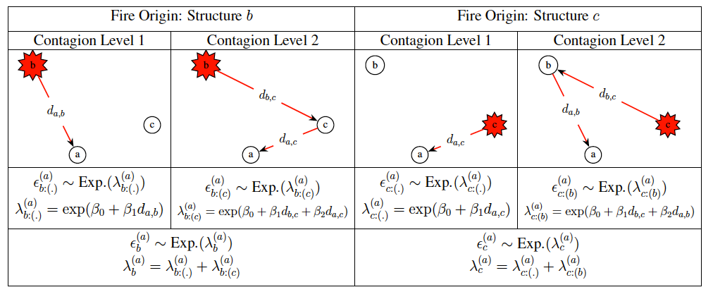
Figure 3 illustrates all contagion processes that ultimately touch structure $a$. For example, we can see that, when the fire originates in structure $b$, as we have only $J = 3$ structures in the farm, $J - 1 = 2$ contagion levels are possible:

1. a level 1 contagion, where the fire passes directly from $b$ to $a$

2. a level 2 contagion, where the fire takes an indirect path, passing from $b$ to $c$ and then going from $c$ to $a$

Figure 3.All contagion processes for a farm with 3 structures

We refine our notation of the contagion associated with these two levels as we introduce $I^{(a)}_{b:(.)}$ and $I^{(a)}_{b:(c)}$ respectively, where the subscript of each random variable $I$ represents the origin of the fire, followed in parenthesis by the path used by the fire before finally touching structure $a$ (in superscript). In summary, according to this figure, we obtain the following two probabilities of contagion:

$$\begin{aligned} \Pr(I^{(a)}_{b} = 1) = F_{\epsilon^{(a)}_{b}}(1; \lambda^{(a)}_{b}) = 1 -\exp(- \lambda^{(a)}_{b}) \\ \Pr(I^{(a)}_{c} = 1) = F_{\epsilon^{(a)}_{c}}(1; \lambda^{(a)}_{c}) = 1 -\exp(- \lambda^{(a)}_{c}). \end{aligned}$$

By setting values to all parameters needed, it then becomes possible to compute the premium for this example. In Table 1, the values of all $\beta$ parameters, all distances, all expected fire frequencies (meaning a fire that starts in the structure), and all expected severities (from direct fire) are shown.^[3]

The resulting values are shown in Table 2, from which we see that several interesting measures can be defined. First, the variable $E[N^{(s)}]$ is defined as the expected total number of fires, and corresponds to the expected number of times a structure $s$ will be touched by fire (direct or contagion). This value is computed as:

$$\begin{aligned} E[N^{(s)}] = E[I_{a}^{(s)}] E[N_a] + E[I_{b}^{(s)}] E[N_b] + E[I_{c}^{(s)}] E[N_c]. \end{aligned}$$

We can also compute the frequency contagion impact for structure $s$, denoted by $FCI(s)$, defined as the ratio between the expected total number of fires for structure $s$ divided by the expected total number of fires beginning in structure $s$. Formally, it corresponds to

$$\begin{aligned} FCI(s) &= \frac{E[N^{(s)}]}{E[N_{s}]}. \end{aligned}$$

For a given structure $s$, $FCI(s)$ can be interpreted as a measure of relative risk for fire contagion. From Table 2 we see, for example, that structure $a$, which has only a 1% chance of being the origin of a fire, nevertheless has more than a 5% probability of being damaged by a fire. This increase of 542.9% corresponds to the value of $FCI(a)$ and comes mainly from the proximity of structure $a$ to structure $c$. Indeed, the expected number of fires originating in the $c$ structure is 5%, and the $a$ structure has a 63.79% chance of being hit by such a fire. Moreover, the relative risk of fire contagion of structure $b$ is only 169.2%, because structure $b$ is far from both structure $a$ and (mostly) structure $c$.

Finally, we can compute the expected total incurred loss by structure, also called the pure premium by structure. As seen in equation (1), this value is calculated using values of $E[Y^{(s)}_{i}]$, for $i \in \{a, b, c\}$. In other words, it corresponds to the expected severity when the fire is direct or when the fire is from a contagion. Empirical analyses show, as described next in Section 3, that the average severity is lower when fire affects a structure due to contagion. This is not surprising because the cause of the fire is located outside the structure, and, as the fire contagion takes some time to happen, damages resulting from a contagion process can be mitigated (i.e., by firefighter services). We then suppose that:

$$\begin{aligned} E[Y^{(s)}_{x}] = \alpha(x,s) E[Y_{s}] \end{aligned}\tag{4}$$

with $0 \le \alpha(x,s) \le 1$ and $\alpha(s,s) =1$. That means the expected severity from contagion is a proportion of the expected severity from a direct fire. For the purpose of illustration, we will suppose that $\alpha(x,s) = 25\%$ for $s \ne x$. We can then adapt equation (1) as:

$$\begin{aligned} E[S^{(s)}] &= E[I_{a}^{(s)}] E[N_a] E[Y^{(a)}_{a}] \\ &\quad+ E[I_{b}^{(s)}] E[N_b] E[Y^{(s)}_{b}] \\ &\quad+ E[I_{c}^{(s)}] E[N_c] E[Y^{(s)}_{c}] \\ &= E[I_{a}^{(s)}] E[N_a] \left( \alpha(a,s) E[Y_{s}] \right) \\ &\quad+ E[I_{b}^{(s)}] E[N_b] \left( \alpha(b,s) E[Y_{s}] \right) \\ &\quad+ E[I_{c}^{(s)}] E[N_c] \left( \alpha(c,s) E[Y_{s}] \right). \end{aligned}$$

For each structure $s$, and similar to $FCI(s)$, we also introduce the pure premium contagion impact, $PCI(s)$, defined as

$$\begin{aligned} PCI(s) &= \frac{E[S^{(s)}]}{E[S_{s}]} = \frac{E[S^{(s)}]}{E[N_{s}] E[Y_{s}]}. \end{aligned}$$

We can see that the inclusion of the severity in the computation of the risk contagion decreases the overall impact of the contagion. Indeed, analyses of the variable $FCI(s)$ show that contagion risk only increases the pure premium by 8% for structure $c$, while the contagion impact for structure $a$ goes from 542.9% to 210.7% when the severity is considered.

We have thus far considered each structure individually, which allows us to compute the total frequency for a given farm as well as its total pure premium. The expected number of structures touched by a fire for this farm is 17.23%, for a corresponding FCI equal to 191.3%. We must be careful in interpreting the frequency as it is based on three structures, meaning that a single fire can impact up to three structures at the same time. For the pure premium, we obtain a value of $3,653.13$, for a corresponding $PCI$ of 117.8%, meaning that the contagion risk only increases the pure premium by 17.8% for the farm, despite the high probability of fire contagion. Obviously, higher values of $\alpha(x,s)$ could significantly increase the impact of fire propagation.

2.2.2. Distances and levels of contagion

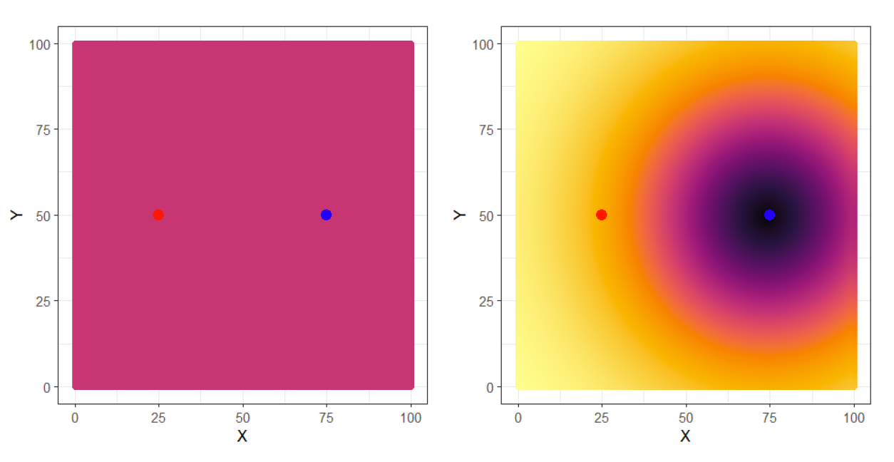
We can generalize the last example to better understand how the layout of structures on a farm impacts each level of contagion. We then suppose a $100 \times 100$ coordinate plane where structure $a$ is located at $(75, 50)$ (i.e., the blue dots in Figures 4–6) and structure $b$ (the red dots) at $(25, 50)$. Next, we place a third structure $c$ at all possible locations in the plane to see how it impacts$E[N^{(a)}]$. The values of $\beta$ from the previous example are kept.

Figure 4 illustrates the probability of level 1 contagion according to the location of the structure $c$ and the structure of origin for the fire. We see that the location of the $c$ structure has no influence on the level 1 contagion when the source of the fire is structure $b$, which is logical. In addition, as one might expect, when the origin of the fire is the structure $c$, the level 1 contagion is higher when $c$ is located near structure $a$.

Figure 4.Level 1 contagion for structure a (blue dot), depending on the location of structure c (left: origin of the fire is structure b (red dot), right: origin of the fire is structure c)

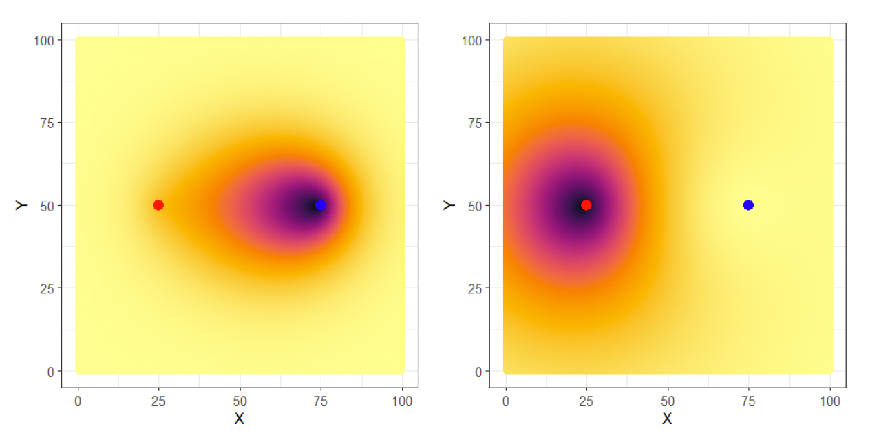
Figure 5 illustrates the probability of level 2 contagion, again according to the location of structure $c$. Unlike level 1 contagion, we notice that the location of structure $c$ strongly influences level 2 contagion when the origin of the fire is structure $b$. The risk is more important when $c$ is between structure $a$ and structure $b$, which indeed facilitates the propagation of a fire starting in $b$, traveling to structure $c$, and ultimately impacting structure $a$. Similarly, when the origin of the fire is structure $c$, the level 2 contagion risk will be greater when $c$ is located so that $b$ is between $c$ and $a$, which also facilitates contagion.

Figure 5.Level 2 contagion for structure a (blue dot), depending on the location of structure c (left: origin of the fire is structure b (red dot), right: origin of the fire is structure c)

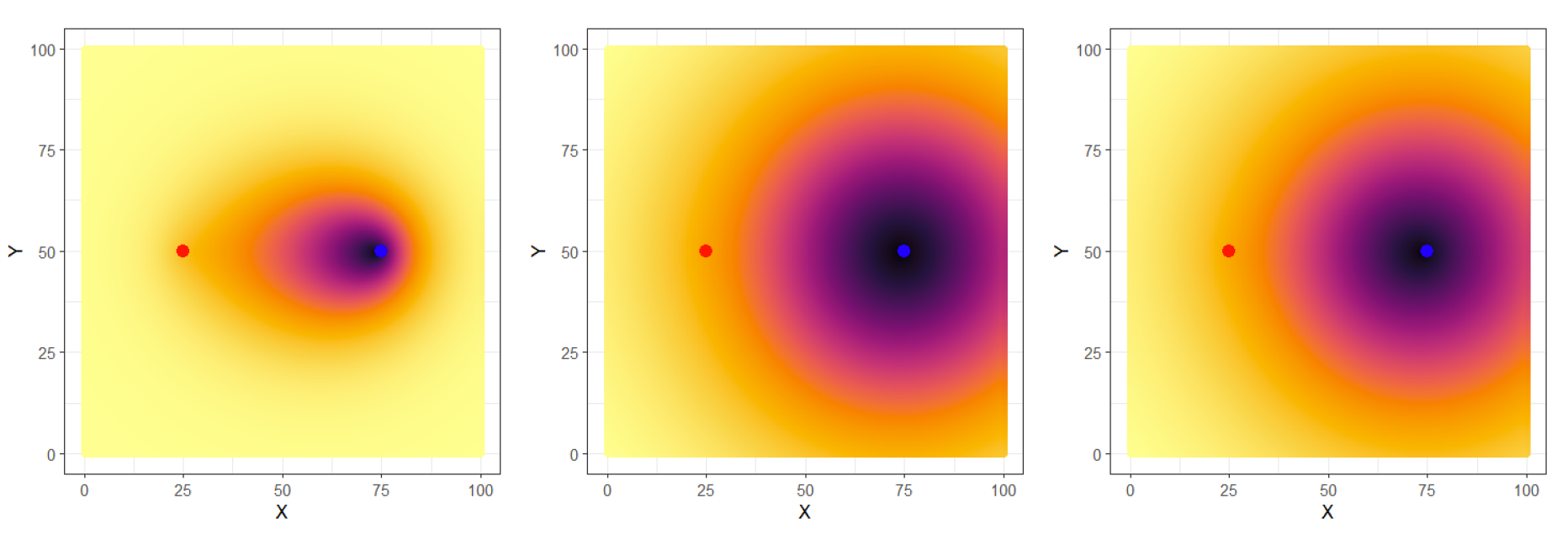
The combination of level 1 and level 2 contagions is illustrated in Figure 6. Depending on the $\beta$ parameters chosen, the importance of level 1 and level 2 contagions on the total contagion risk will be different. In our example, we can see that the level 1 contagion is much more important than the level 2 contagion. Finally, assuming the same probability that a fire starts in structure $b$ or $c$ ($E[N_{b}] = E[N_{c}]$), the right plane in Figure 6 illustrates the total contagion risk of structure $a$ depending on the location of structure $c$.

Figure 6.Total contagion risk for structure a (blue dot), depending on the location of structure c (left: origin of the fire is structure b (red dot), middle: origin of the fire is structure c, right: both origins combined)

3. Empirical example and data inference

We use a subset of data from a Canadian insurance company to apply the contagion model to farm insurance data (December 2013 to December 2019). For each insurance policy, the number of structures on each farm as well as a detailed description of each structure were available. This included, for example, its type, usage, year of construction, size, and so on. For each fire claim, we were able to identify in which structure the fire originated and the damages to all structures. Usually, the characteristics of each contract allowed us to estimate the parameters associated with the frequency and the severity of a claim. We observed 5,251 claims during this six-year span, including 466 fire claims.

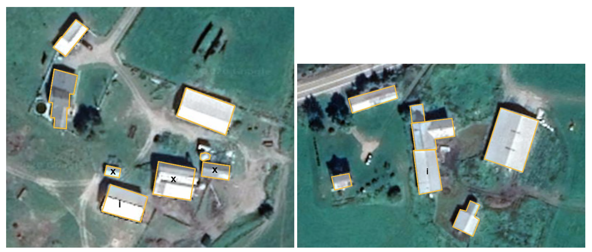
However, this kind of dataset cannot be used directly to model the contagion processes. Indeed, we do not have the coordinates of all structures for each farm, nor a $J \times J$ distance matrix showing the distances between all $J$ structures of a farm. Instead, we took a sample of 39 farms with fire damages from which detailed analysis was done. On an individual basis, we identified the physical disposition of all structures for each farm using the address of the farm and images from Google Earth. For each claim, we also identified the structure from which the fire originated, as well as the structures damaged by the fire. To give two examples, Figure 7 illustrates structures from two Canadian farms^[4] selected randomly from Google Earth. To illustrate how we constructed our database of 39 farms, we show how the fire information was added to our images. Thus, the letter $I$ is used to identify the structure of origin, and $X$ indicates which structures have been damaged by the fire. The picture on the left of Figure 7 shows fire propagation, while the picture on the right shows a fire without contagion.

Figure 7.Example of farms with fictive fire damages. Left: with fire contagion, Right: without fire contagion ($i$ corresponds to fire origin, $X$ corresponds to damaged structures)

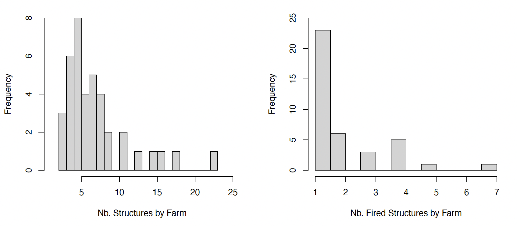
The 39 farms studied had a total of 288 structures, for an average of 7.38 structures per farm, with a standard deviation of 4.42. The smallest number of structures observed on the same farm was 2, while the largest number of structures on a farm was 23. Figure 8 (left) shows a histogram of the number of structures per farm. On average, for each farm fire, 1.95 structures were touched (for a standard deviation of 1.45). The minimum number of structures affected for a single fire was 1, corresponding to a fire exhibiting no propagation. For 23 of the 39 fires selected, representing 59% of the fires, we did not observe fire propagation. Conversely, the maximum number of structures affected for a single fire was 7. Figure 8 (right) shows the histogram of the number of structures affected by fire. In relation to the number of structures on a farm, on average 33% of structures were damaged when a fire occurred, with a minimum of 4% (1 structure out of 23), and a maximum of 80% (4 out of 5 in total).

Figure 8.Histogram of the number of structure by farm (left), and number of damaged structure by fire claim (right)

Figure 9 illustrates how we interpret the layout of a farm. It shows how easy it is to determine the minimum distance between the structures. In contrast to the theoretical contagion approach developed earlier, each structure does not correspond to a point, but rather to a polygon in plane. However, it becomes simple, as illustrated on the right side of the same figure, to transform the farm into one summarized by points, where the (minimum) distances between structures ($d_i, i = 1, \ldots, 6$) are kept. Although it is important to remember the difference in the diagram of a farm made up of points vs. polygons, we believe that the theoretical approach correctly approximates the situation.

Figure 9.Farm Example

3.1. Inference

Even with data that included distances between structures, the estimation of the parameters of the contagion model remains a procedure which requires a good understanding of the competing contagion processes. The contagion processes, which follow an exponential distribution, have a parameter which depends on the level of contagion and the distances between the structures, as indicated by equation (3).

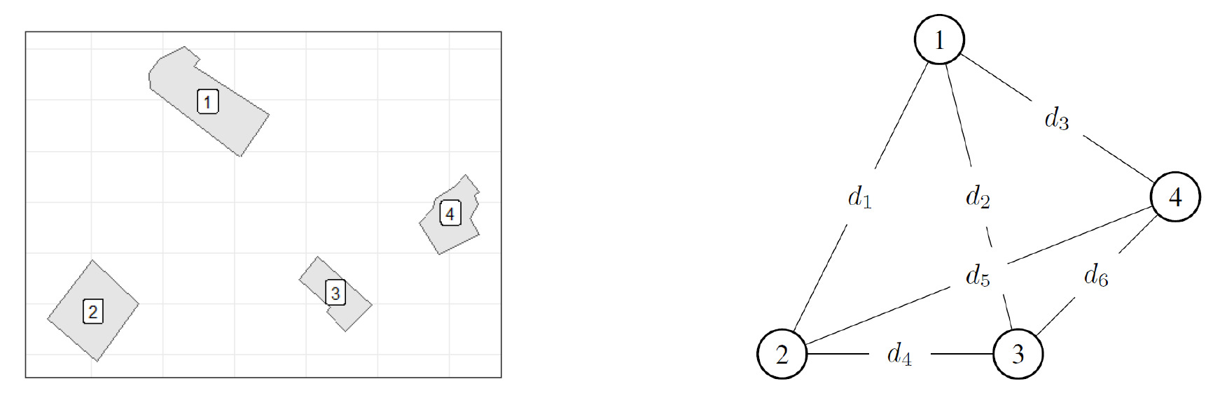
When we observe a fire on a farm, whether there is contagion or not, several contagion processes are observed and are often in competition. Other processes are simply not activated at all and are therefore not observed. To better understand the difference between the contagion processes observed and those that are not observed, a simple example is made from a farm with four structures. We will assume:

• the origin of the fire is structure 2;

• structures 1 and 3 are affected by the fire (we don’t know in what order); and

• structure 4 is spared and is not affected by the fire.

With this information, it becomes easier to identify processes that are not activated (in other words, unobserved). Indeed, with structure 2 being the origin of the fire, all the contagion processes beginning with structures 1, 3, or 4 are not activated. On the other hand, all the contagion processes starting with structure 2 will be observed, and some will even be competing with each other.

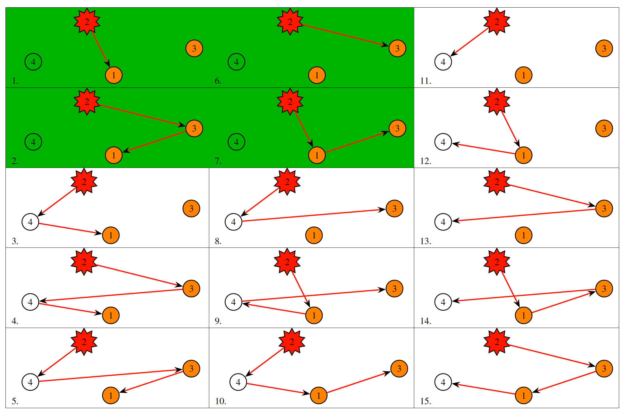
Among the observed processes, we will be able to determine which processes are possible and which are impossible. With four structures, we observe 15 potential processes, shown in Figure 10. Each column of the table in this figure represents which structure is analyzed: column 1 considers what happens to structure 1, column 2 considers what happens to structure 3, and column 3 considers what happens to structure 4. Only the processes in green, numbered 1 and 2 (for the analysis of structure 1), or 6 and 7 (for the analysis of structure 3) are possible. The other processes cannot have taken place since they involve contagion to structure 4, which we know was spared.

Figure 10.Illustration of the 15 contagion processes observed for a farm having 4 structures

Such an enumeration of all the processes observed, by identifying the impossible processes and those in competition, must be made for all the fires recorded, assuming a maximum number of levels of contagion. Indeed, knowing that we have observed a farm with 23 structures, the number of possible contagion processes in such a situation is of the order of 23! which greatly exceeds computing resources. Thus, in our case, we have limited the number of possible contagions to four (i.e., level 3 contagion). This implies that a fire can only affect a maximum of two other structures before spreading to the structure under study. We consider this hypothesis to be in no way restrictive because level 1 and level 2 contagions are still possible. With the 39 fires studied, we obtain a database listing 25,907 possible contagion processes.

In connection with the modeling proposed earlier and equation (2), an impossible contagion process necessarily implies that its associated $\epsilon$ r.v. is greater than 1. On the other hand, it is important to remember that a possible process does not necessarily imply that its associated $\epsilon$ r.v. is less than 1. Indeed, as described earlier, contagion processes are in competition. When we examine structure 1, processes 1 and 2 are in competition, and processes 6 and 7 are in competition when we examine structure 3. Tables 3 and 4 summarize how the impossible processes and competing processes can be represented by the previous example. The associated probability, in relation to the log-likelihood (yet to computed), is also indicated in the tables.

3.1.1. Log-likelihood

Regarding the database with 39 farm fires, among the $25,907$ contagion processes listed, $25,618$ processes are considered impossible. Using the distances and equation (3), it is therefore possible to calculate the value of the $\lambda$ of each impossible process, and to calculate the contribution to the log-likelihood:

$$\begin{aligned} \ell_1 = \sum_{i=1}^{25,618} \log(\Pr(\epsilon_i > 1)) = \sum_{i=1}^{25,618} 1- \lambda_i. \end{aligned}$$

This leaves only 289 possible processes, which often compete with each other. By also using distances between structures and equation (3), we need to calculate the value of $\lambda$ for each process. Because processes are in competition, the distribution of the minimum must be found, corresponding to an exponential distribution with a parameter equal to the sum of $\lambda$. When we account for the 289 possible processes, we obtain 37 competitions between processes. The contribution to the log-likelihood of the model for these observations can now be calculated and is expressed as:

$$\begin{aligned} \ell_2 = \sum_{i=1}^{37} \log(\Pr(\epsilon_i < 1)) = \sum_{i=1}^{37} \log(1 - \exp(1- \lambda_i)) \end{aligned}$$

where $\lambda_i$ corresponds to the sum of $\lambda$ from possible processes. For the model, we then obtain the following log-likelihood:

$$\ell = \ell_1 + \ell_2.$$

Maximizing the log-likelihood will thus allow to obtain estimates of all model parameters.

3.1.2. Estimation results

We have thus estimated the parameters of the proposed model. We have tested some model formulas for $\lambda$, more specifically the following possibilities:

$$\begin{aligned} \lambda^{lin} &= \exp(\beta^{lin}_0 + \beta^{lin}_1 d_1 + \beta^{lin}_2 d_2 + \beta^{lin}_3 d_3) \\ \lambda^{log} &= \exp(\beta^{log}_0 + \beta^{log}_1 \log(d_1) + \beta^{log}_2 \log(d_2) + \beta^{log}_3 \log(d_3)) \\ \lambda^{sqr} &= \exp(\beta^{sqr}_0 + \beta^{sqr}_1 \sqrt{d_1} + \beta^{sqr}_2 \sqrt{d_2} + \beta^{sqr}_3 \sqrt{d_3}) \end{aligned}$$

where $d_3$ is missing for a level 2 contagion, and $d_2$, $d_3$ are missing for a level 1 contagion. The result of the parameter estimation is shown in Table 5. We see that the model based on the logarithm of distances and the one based on the square root of distances seem to be more adequate than the linear model. The difference in the quality of the fit, related to the log-likelihood, is small between the log model and the square-root model. The standard deviation of the parameters shows that only level 1 contagions are statistically significant. With 39 fires, most of them without contagion, it is not surprising to obtain such a result. It would be interesting to amend the current dataset to obtain further results.

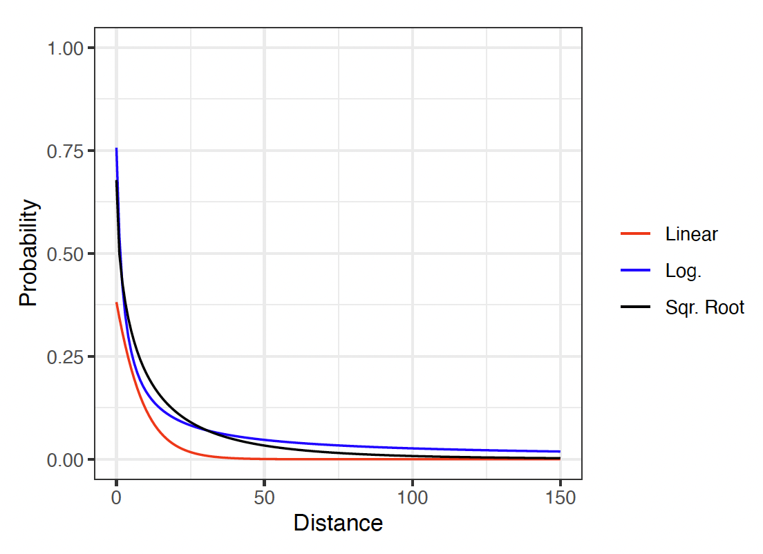
The relationship between the probability of contagion and the distance, for a level 1 contagion, is illustrated in Figure 11. We see a similarity between the logarithmic and square-root models, whereas the linear approach is different. As opposed to Pesic et al. (2017), previously cited, the model seems to show that fire contagion is possible between structures which are more than 10, 25, or even 50 meters apart. This conclusion, even if it is in opposition to the results of Pesic and colleagues, is not surprising, because we already saw in our portfolio that fire contagion between structures located relatively far from each other is possible.

Figure 11.Link between distance and contagion probability (level 1)

3.2. Examples

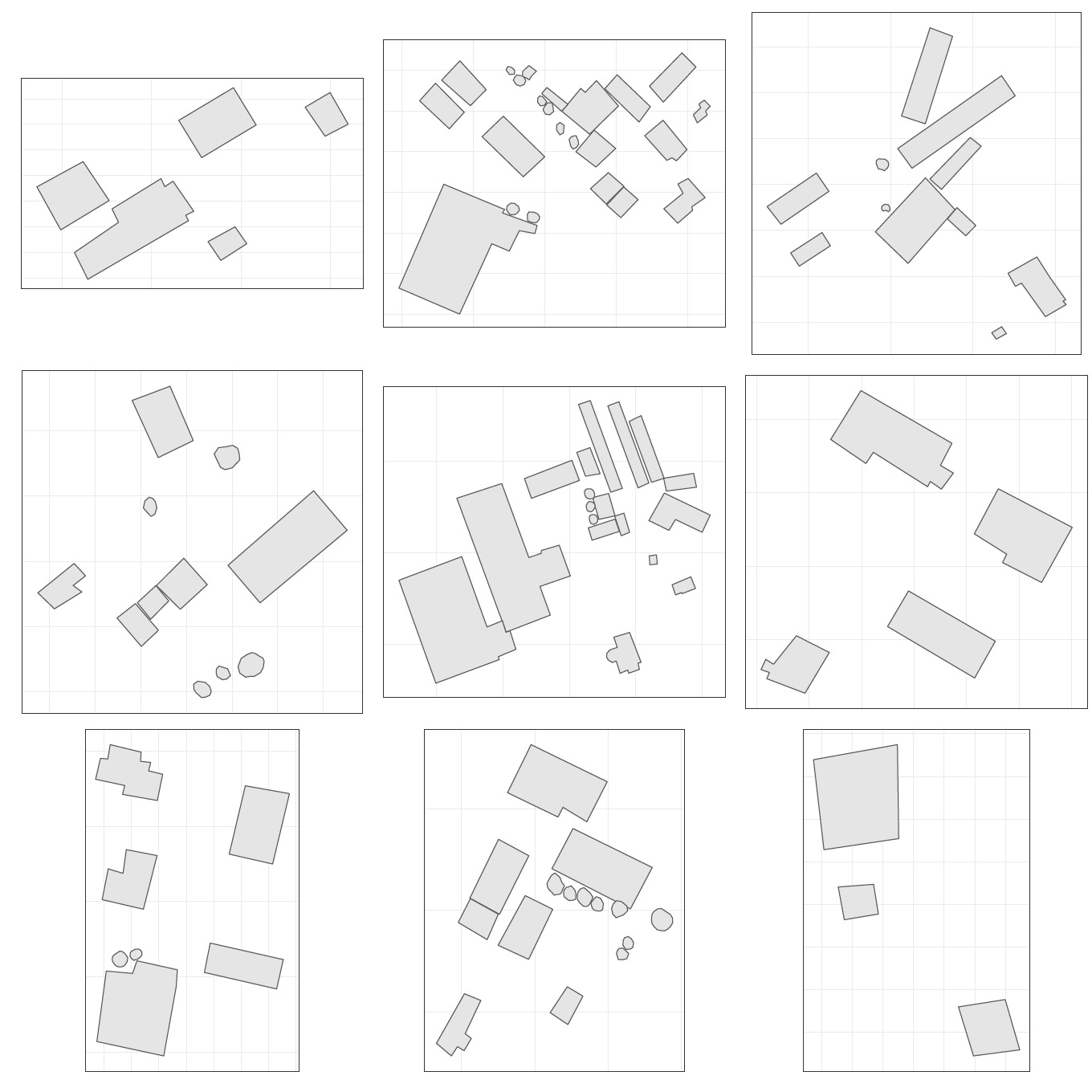
The proposed model makes it easy to estimate the risk of contagion for each structure on a farm, by considering the different possible levels of contagion and the distances from other structures. By setting values for $E[N_j], j = 1, \ldots, J$, the expected number of fires which begin in structure $j$, as well as $E[Y^{(s)}_{j}]$, the expected severity to structure $s$ when the fire originates from structure $j$, we will be able to compute a premium for each structure of the farm, and for the farm as a whole. In order to illustrate the model presented in this paper, we will take nine farms as examples, all illustrated in Figure 12. We must, however, be careful in analyzing this figure since the diagrams are not all at the same scale. Using those diagrams, we will show how the proposed model determines the contagion probabilities for each structure.

Figure 12.Diagram of farms #1 to #9

3.2.1. Contagion probabilities

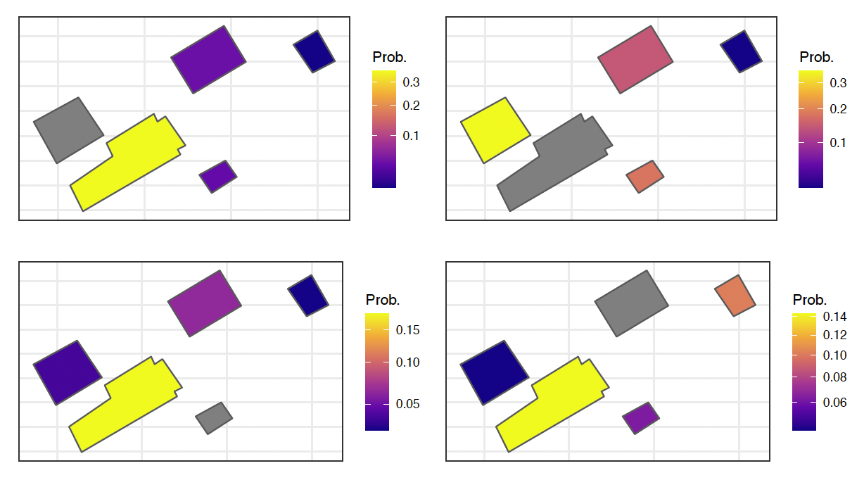
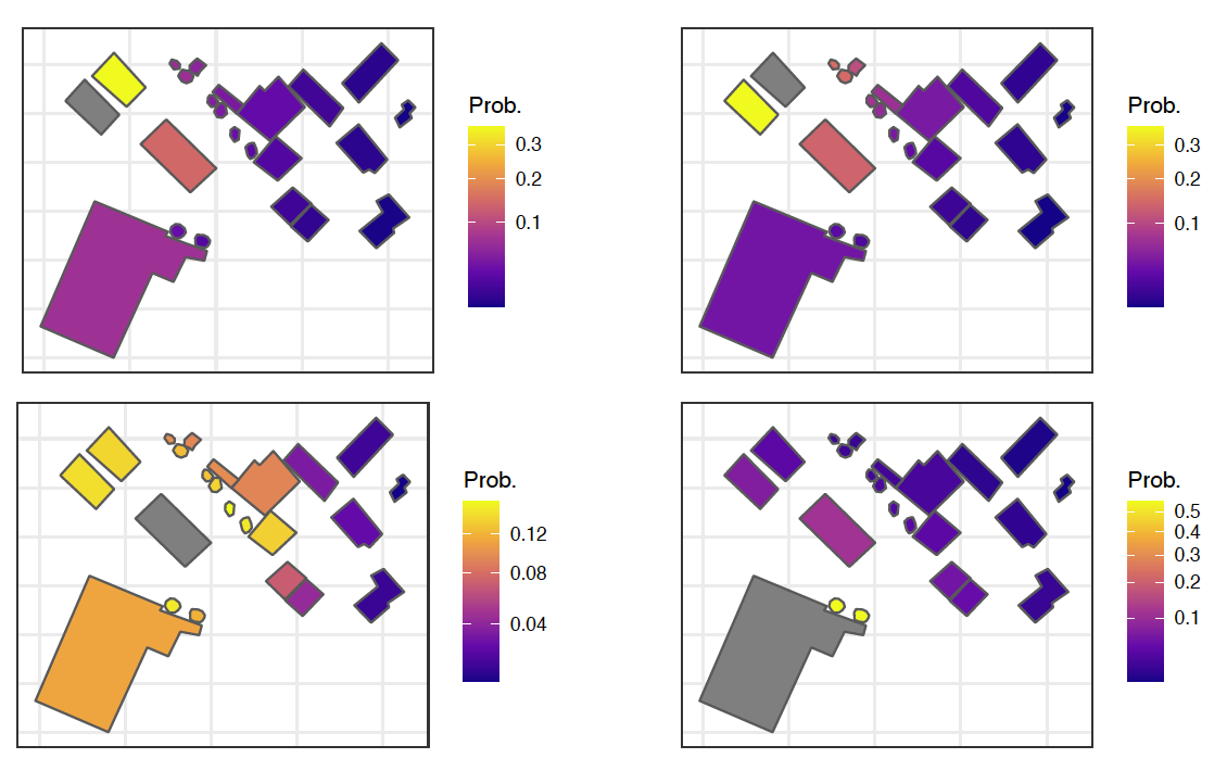
Farm #1 is the simplest farm to use to illustrate the model, as it has only five structures. For this farm, Figure 13 illustrates how the model computes contagion probabilities, with the square root of distances between structures as predictors, where the estimated parameters used are from Table 5. For each of these farms, each of the structures were evaluated, where the chosen structure appears in gray. The colors of the other structures correspond to the probability of the contagion. If we take the upper left diagram of Figure 13 for example, we can see that if a fire originates from the structure in yellow, there is more than a 30% chance of it spreading to the gray structure. On the opposite, if the structure of origin is the structure in blue, there is almost no chance that the structure in gray will be damaged (for any contagion level). A similar illustration of probabilities has been done for farm #2, in Figure 14.

Figure 13.Diagram of a farm: Probability of contagion according to the structure being evaluated (in grey) - Farm #1

Figure 14.Diagram of a farm: probability of contagion according to the evaluated structure (in grey) - Farm #2

For each structure on the farm, we must then evaluate the risk of fire based on the possibilities that a fire can start in any structure. For any farm, we define the total risk as a function that has as its arguments all of the structures on a farm (not only the first four structures, as in the example).

3.2.2. Impact of contagion and premiums

It should be noted that the proposed model, as we indicated at the beginning of this paper, mainly focuses on contagion. Thus we can see for farm #2, in the lower right square of Figure 14, that the largest structure on the farm is highly at risk ($> 50\%$) of being damaged by a fire that impacts one of the two adjacent silos. If we only consider contagion, this structure could be considered risky, compared to a similar structure that is isolated from those silos. However, to fully understand its level of risk, we should also consider the probability that a fire starts in a silo. Indeed, knowing that a fire starting in a silo is a rare event compared to a fire starting in an animal barn, the risk thus becomes much lower.

To illustrate in a somewhat more realistic way how we can use the contagion model, we have made the following additional assumptions:

1. $N_j$, the number of fires that start in structure $j$ (by year), is proportional to the size of the structure. Formally, we have $E[N_j] \propto$ area of the structure in $m^2/1000$.

2. As defined in equation (4}), we will suppose that $E[Y_{s}] = 1$ and $\alpha = 0.25$. That means the severity of a direct fire is equal to 1, while the severity of a fire from contagion is equal to 0.25.

We do not have enough data to formally verify those assumptions. However, based on our discussions with claims adjusters and experts, they seem plausible. In any case, they are only used here to explain how the contagion model could potentially be used.

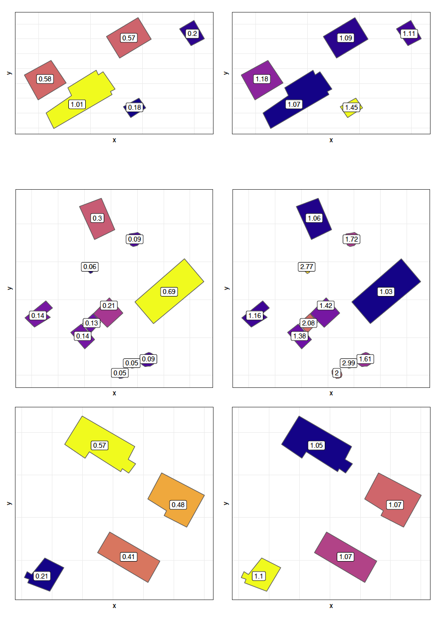
We are now able to compute the impact of fire contagion on frequency by structure through $FCI(s)$. Based on equation (1), we are now able to compute the premium

$$\begin{aligned} E[S^{(a)}] &= E[N_a]E[Y_a^{(a)}] + \alpha \sum_{k=1, k\ne a}^J E[N_k] E[Y_k^{(a)}], \end{aligned}$$

from which the premium contagion impact of each structure ($PCI(s)$) can also be computed. We use farms #1, #4, and #6 to illustrate the situation. The left part of Figure 15 shows the premium of each structure without considering the fire contagion, while the right part shows the premium contagion impact for each structure. For farm #1, in the left part of that figure, we see that the largest structure has a higher premium when we do not consider contagion. This was expected because the structure is large, and we create the model by supposing that $E[N_j]$ is proportional to its size. To the right we see, however, that considering the fire contagion for that structure increases the level of risk by only 7%. On the other hand, the smallest structure of that farm is at risk for fire contagion. Because it is located near the largest structure, its probability of being damaged by a fire increases by 45%.

Figure 15.Left: Premium for each structure without contagion, Right: Premium contagion impact of each structure (First line: farm # 1, second line: farm #4 , third line: farm #6)

Farm #4 is interesting to analyze because it has a lot of small structures. We see from the second line of diagrams in Figure 15 that the presence of those small structures near the larger one only generates a $PCI$ of 103% for this large structure. On the opposite, small structures are always greatly impacted when they are close to a large structure. Based on our assumptions, premiums for those structures of that farm should be doubled. Finally, farm #6 can be analyzed similarly. This farm has four structures, all far from each other. The risk of fire propagation is then low. This can be observed from the resulting $PCI$ for each structure, where the largest value is 110% for the smallest structure of the farm. Note that, even if not illustrated here, more extreme situations can arise. For example, premiums for silos near the largest structure of farm #2 are 10 times larger when we consider fire contagion.

As done previously in Section 2.2.1, by summing the premiums of all structures for a farm, we can also compute the total premium associated with the fire peril, as well as the premium contagion impact of the farm. Table 6 shows the details for all nine farms. We can see the total number of structures for each farm, the sum of losses from direct fire ($\sum_{j=1}^J E[S_s]$), and the sum of losses when fire contagion is considered. The last column, $PCI$ (pure premium contagion index), represents the ratio of the two last values and is a measure of the risk of fire contagion. We can see that farm #2 is the riskiest, because the consideration of fire contagion increases its premium by 54.6%. Figure 12 can explain this result, because it shows us that this farm has a lot of adjacent structures, and large structures are sometimes close to each other. For the same reason, farms #5 and #8 are also very risky. Farms #6 and #9, on the other hand, only need an increase of 6.7% and 5.4% if the insurer wants to consider fire contagion. This is not surprising because those farms have a small number of structures, and they are far from each other. Overall, by comparing the results of this table with all the farm diagrams of Figure 12, results obtained are logic and coherent.

4. Discussions: Future improvements

4.1. Dependence and common contagion processes

The theoretical model developed, although giving very satisfactory results and being very flexible, is obviously not perfect. The approach allows a fire frequency and a premium to be calculated, but it is not easy to determine the overall dependence between the fire damages of structures. Indeed, the modeling is done independently for each structure. That means all contagion processes associated with one structure are independent of the contagion processes of another structure.

For example, let us take all 15 processes of Figure 10. Processes 1 and 2 are competing processes when evaluating structure 1, and processes 6 and 7 are competing structures when evaluating structure 3. However, these two competitive pairs of processes should not be described independently of each other. Indeed, there is a clear dependence between them: only combinations of processes 1 and 7 (when we suppose that the path of the contagion between structures is $2 \rightarrow 1 \rightarrow 3$) or 2 and 6 (when we suppose the path is $2 \rightarrow 3 \rightarrow 1$) are possible. For the computation of the premium, based on the expected value here, the approach proposed in the paper is still correct. However, if we want to assess the overall risk distribution of a farm by considering the risk distribution of all structures simultaneously, improvements must be made. Further research is underway to see how it might be possible to generalize the approach developed here.

4.2. Blocked contagions

There are some farms where the approximation of a polygon by a point is not entirely realistic. For example, structure D in Figure 16, which can represent a silo, is isolated from a level 1 contagion for fires starting in structures A or B. In fact, only a level 2 or level 3 contagion, affecting at least structure C, is a risk for structure D. To be more precise in the analysis of contagion, it would probably be necessary to eliminate the direct contagions between A and D and between B and D, in the statistical inference of the parameters and in the pricing. In this case, these limitations would generate the following consequences:

1. No level 1 contagion between the couples $(A, D)$, $(B, D)$

2. No level 2 contagion for the paths $(A, B, D)$, $(B, A, D)$, $(C, B, D)$, $(C, A, D)$

3. No level 3 contagion for the paths $(C, A, B, D)$, $(C, B, A, D)$

Figure 16.Diagram of a farm where some structures block potential contagion between other structures

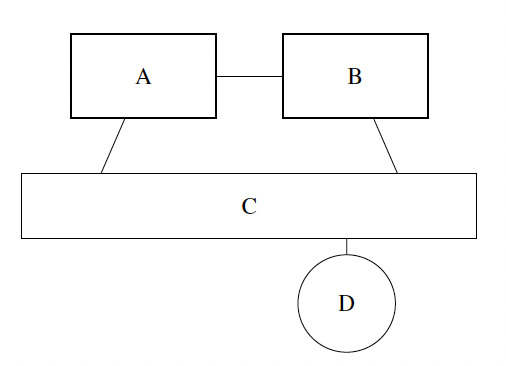
It would probably be possible to manually identify all the levels of contagions that are impossible. However, this task is very labor intensive. Instead, it would probably be better to see if computer tools are already available that can carry out such a task automatically. Considering the 39 farms chosen, however, we see that the cases of contagion that should be canceled are rare, and probably not very important. Indeed, many of the contagion paths that needed to be blocked are due to structures that are already great distances apart, meaning that the probability of contagion was already close to zero. Moreover, as we are observing farm layouts in two dimensions, the height of each structure is not considered. For example, silo D of Figure 16 may seem to be blocked from level 1 contagion from structure A and B, but the contagion may still be possible when height is considered. Overall, even if some improvements can be done for blocked contagion, we believe that the suggested approach remains realistic.

5. Conclusion

The proposed approach has to be seen as a first step in modeling fire contagion between structures. We use an example in farm insurance. We show how images from Google Earth can be useful in modeling fire contagion. The introduction of exponential contagion processes, inducing competition between processes, is an idea that allowed us to easily model all contagion levels. This also allowed us to correctly estimate the parameters of the model, making an appropriate selection of unobserved processes. Ultimately, we can also determine the processes that indicate a fire propagation and those that do not. With any matrix of distances between structures, it is possible to easily calculate a premium for each structure on the farm, as well as an overall premium for the farm. The model also allows us to compute contagion factors that permit the insurer to identify which structures are (relatively) riskier. Its computation speed and its ease of interpretation ensure the simple application of this approach (provided distance matrices are available). In the last section of the article, future improvements have been proposed to generalize the proposed model. Application with larger datasets could be interesting but would probably involve other kinds of problems, as only 39 farms with fires involve almost 26,000 contagion processes. Simulation studies to analyze the loss distribution of the whole portfolio might also be interesting.

Acknowledgments

The authors gratefully acknowledge The Co-operators through the Co-operators Chair in Actuarial Risk Analysis. The authors would like to thank the reviewers for their thoughtful comments and efforts toward improving our manuscript.