Bayesian Predictive Modeling for Exponential-Pareto Composite Distribution

1. Introduction

Two important operations in actuarial science—using data to construct a model and estimating parameters of interest based on the model—are used in the insurance industry. In this paper, both processes are presented in the context of a composite distribution.

Because insurance data is skewed via a fat tail, it is very difficult to find a classical parametric distribution to model data. The central limit theorem is not very useful for the insurance industry because insurance data usually has high frequencies for small losses, and large losses occur with small probabilities. Therefore, many researchers have developed composite models for insurance data or data with similar characteristics. Klugman, Panjer, and Willmot (2012) discussed how to use data to build a model in the actuarial science field and the insurance industry, including many important concepts, such as value at risk (VaR). VaR, one of the most important risk measures in the business world, is the percentile of the distribution of losses. It lets actuaries and risk managers look at “the chance of an adverse outcome” and helps them to make a decision. This paper uses Bayesian inference to estimate VaR based on a predictive model.

Teodorescu and Vernic (2006) introduced the composite exponential-Pareto distribution, which is a one-parameter distribution. They derived a maximum likelihood estimator for the unknown parameter θ, which represents the boundary between small and large losses in a data set. In a subsequent paper, the same authors worked on different types of exponential-Pareto composite models (Teodorescu and Vernic 2009). Both models have one unknown parameter. Researchers have proposed many other composite distributions. Preda and Ciumara (2006), for example, introduced the Weibull-Pareto and lognormal-Pareto composite models, pointing out that they could be used to model actuarial data collected from the insurance industry. The authors compared the models using different parameters, developed algorithms to find the maximum likelihood estimates for two unknown parameters, and compared the two models’ accuracy.

Pareto distribution has a fatter tail than normal distribution. Therefore, Pareto is a good model to capture large losses in insurance data, but it is not good for small losses with high frequencies. That is why many other distributions, such as exponential, lognormal, and Weibull, have been combined with the Pareto distribution to model losses with small values in a data set. Cooray and Ananda (2005) discuss modeling actuarial data based on a composite lognormal-Pareto composite model. Cooray and Cheng (2015) provide Bayes estimates for parameters of a lognormal-Pareto composite model. Scollnik and Sun (2012) discuss several Weibull-Pareto composite models.

The aim of this paper is to develop a Bayesian predictive density based on the composite exponential-Pareto distribution. In the Bayesian framework, a predictive density is developed via the composite density and then, based on a random sample, a Bayes estimate and the VaR are estimated. The following section develops a posterior probability density function (pdf) via an inverse gamma prior for θ. It also explains how to use a search method to compute the Bayes estimate for θ based on a sample. Section 3 derives the predictive density for Y, where its realization, y, is considered as a future observation from the composite distribution. The first moment, E[Y|x], of the predictive pdf is undefined because E[X] is also undefined for the composite pdf. Section 4 investigates the accuracy of VaR and shows, through a summary of simulation studies, that Bayes estimation of θ under a squared error loss function is consistently more accurate than maximum likelihood estimation (MLE). The section also gives a method for choosing the “best” values for hyperparameters of the prior distribution to get an accurate Bayes estimate. Section 5 contains a numerical example for computational purposes. Three Mathematica codes are given in the Appendix, one for computing the MLE of θ, the second for computing a Bayes estimate and VaR using a single sample, and the third for a simulation that can be used to search for the “best” values of hyperparameters to find an accurate Bayes estimate.

Teodorescu and Vernic (2006) developed the composite exponential-Pareto model as follows:

Let X be a random variable with the pdf

$$f_{x}(x)=\left\{\begin{array}{ll} c f_{1}(x) & 0<x \leq \theta \\ c f_{2}(x) & \theta \leq x \leq \infty \end{array}\right.,$$

where

$$f_{1}(x)=\lambda e^{-\lambda x}, x>0, \lambda>0$$

and

$$f_{2}(x)=\frac{\alpha \theta^{\alpha}}{x^{\alpha+1}}, x \geq \theta$$

f₁(x) is the pdf of an exponential distribution with parameter λ, and f₂(x) is the pdf of a Pareto distribution with parameters θ and α.

In order to make the composite density function smooth, it is assumed that the pdf is continuous and differential at θ. That is,

$$f_{1}(\theta)=f_{2}(\theta), f_{1}^{\prime}(\theta)=f_{2}^{\prime}(\theta).$$

Solving the above equations simultaneously gives

$$\lambda \theta=1.35, \alpha=0.35, c=0.574.$$

As a result, the initial three parameters are reduced to only one parameter, θ, for the composite exponential-Pareto distribution whose pdf is given by

$$f_{x}(x \mid \theta)=\left\{\begin{array}{ll} \frac{.775}{\theta} e^{\frac{-1.35 x}{\theta}} & 0<x \leq \theta \\ \frac{.2 \theta^{.35}}{x^{1.35}} & \theta \leq x<\infty \end{array}\right. \text {. } \tag{1.1}$$

Figure 1.1 provides graphs of the composite pdf for different values of θ, revealing that as θ increases, the tail of the pdf becomes heavier. This implies that the percentile at a specific level, say 0.99, is increasing in θ. Teodorescu and Vernic (2006) compared the exponential distribution with the composite exponential-Pareto distribution and derived an MLE for θ via an ad hoc procedure using a search method. They concluded that when θ = 10, the composite distribution fades to 0 more slowly than the exponential distribution. The implication of this result is that the composite distribution could be a better choice to model insurance data containing large losses. In this situation, we could be able to avoid charging insufficient premiums to cover potential future losses.

Figure 1.1.Composite pdf for different values of

2. Derivation of posterior density and Bayes estimator

Let x₁, . . . , x_n be a random sample for the composite pdf in (1.1) and, without loss of generality, assume that x₁ x₂ . . . x_n is an ordered random sample from the pdf in (1.1). The likelihood function, also given in Teodorescu and Vernic (2006), is written as

$$L(x \mid \theta)=k \theta^{0.35 n-1.35 m} e^{-1.35 \sum_{i=1}^{n} x_{1} / \theta}, \tag{2.1}$$

where $k=\frac{0.2^{n-m}(0.775)^{m}}{\prod_{i=m+1}^{n} x_{i}^{1.35}}$. To formulate the likelihood function, it is assumed that there is an m(m = 1, 2, . . . , n − 1) such that in the ordered sample x_m ≤ θ ≤ x_m+1.

To derive a posterior distribution for θ, we use a conjugate prior inverse gamma distribution for θ with the pdf

$$\rho(\theta)=\frac{b^{a} \theta^{-a-1} e^{-b / \theta}}{\Gamma(a)}, b>0, a>0. \tag{2.2}$$

From (2.1) and (2.2), the posterior pdf can be written as

$$\begin{aligned} f(\theta \mid x)= & L(\theta \mid x) * \rho(\theta) \propto \\ & e^{-\frac{b+1.35 \sum_{i=1}^{m} x_{i}}{\theta}} \theta^{-(a-0.35 n+1.35 m)-1} . \end{aligned} \tag{2.3}$$

It can be seen from (2.3) that the expression on the right-hand side is the kernel of inverse gamma (A, B), where $A=(a-0.35 n+1.35 m)$ and $B=\left(b+1.35 \sum_{i=1}^m x_i\right)$. Therefore, under a squared error loss function, the Bayes estimator for $\theta$ is

$$\hat{\theta}_{\text {Bayes }}=E[\theta \mid x]=\frac{B}{A-1}=\frac{b+1.35 \sum_{i=1}^{m} x_{i}}{a-0.35 n+1.35 m-1} .$$

Given an ordered sample x₁ x₂ . . . x_n, we need to identify the correct value of m in order to compute $\hat{\theta}_{\text {Bayes }}$. We use the following algorithm:

1. Start with j = 1, and check to see if $x_{1} \leq \frac{B}{A-1} \leq x_{2}$; if yes, then m = 1. Otherwise, go to step 2.

2. For j = 2, check to see if $x_{2} \leq \frac{B}{A-1} \leq x_{3}$; if yes, then m = 2. Otherwise, let j = 3 and continue until the correct value for m has been found.

The idea is to find the correct value for j so that $x_{j} \leq \frac{B}{A-1} \leq x_{j+1}$. The Mathematica code used for simulation studies in this article is based on the above algorithm to compute $\hat{\theta}_{\text {Bayes }}$.

3. Derivation of predictive density

Let y be a realization of the random variable Y from the composite density. Based on the observed sample data x, we are interested in deriving the predictive density f(y|x). In the Bayesian framework, predictive density is used to estimate measures such as E[Y|x] or Var[Y|x], or other measures, such as VaR, which is considered in this paper.

$$f(y \mid x)=\int_{0}^{\infty} f(\theta \mid x) f_{Y}(y \mid \theta) d \theta,$$

where

$$f_{Y}(y \mid \theta)=\left\{\begin{array}{ll} \frac{0.775}{\theta} e^{\frac{-1.35 y}{\theta}} & 0<y \leq \theta \\ \frac{0.2 \theta^{.35}}{y^{1.35}} & \theta \leq y<\infty \end{array} .\right.$$

As a result, we get

$$\begin{array}{l} f(\theta \mid x) f(y \mid \theta) \\ \quad=\left\{\begin{array}{ll} \frac{0.775}{\Gamma(A) \theta} e^{\frac{-1.35 y}{\theta}} \theta^{-(A+1)} B^{A} e^{-B / \theta} & y<\theta<\infty \\ \frac{0.2 \theta^{.35}}{\Gamma(A) y^{1.35}} \theta^{-(A+1)} B^{A} e^{-B / \theta} & 0<\theta<y \end{array},\right. \end{array}$$

which reduces to

$$\begin{array}{l} f(\theta \mid x) f(y \mid \theta) \\ \quad=\left\{\begin{array}{ll} \frac{0.775 B^{A} \Gamma(A+1)}{\Gamma(A)(B+1.35 y)^{A+1}} h_{1}(\theta \mid A+1, B+1.35 y) \\ & y<\theta<\infty \\ \frac{0.2 B^{A} \Gamma(A-.35)}{\Gamma(A) y^{1.35} B^{A-0.35}} h_{2}(\theta \mid A-0.35, B) & \\ & 0<\theta<y \end{array},\right. \end{array}$$

where h₁(θ|A + 1, B + 1.35y) is the pdf of the inverse gamma with parameters A + 1 and B + 1.35y. Also, h₂(θ|A − 0.35,B) is the pdf of the inverse gamma distribution with parameters A − .35 and B. Using the above results, the predictive density, f(y|x), is given by

$$\begin{aligned} f(y \mid x)= & \int_{0}^{y} f(\theta \mid x) f_{Y}(y \mid \theta) d \theta+\int_{y}^{\infty} f(\theta \mid x) f_{Y}(y \mid \theta) d \theta \\ = & K_{2}(y) H_{2}(y \mid A-0.35, B) \\ & +K_{1}(y)\left(1-H_{1}(y \mid A+1, B+1.35 y)\right) \end{aligned}$$

$$\begin{array}{l} K_{1}(y)=\frac{0.775 A * B^{A}}{(B+1.35 y)^{A+1}}, \\ K_{2}(y)=\frac{0.2 B^{.35} \Gamma(A-0.35)}{\Gamma(A) y^{1.35}} . \end{array} \tag{3.1}$$

H₂ is the cumulative density function (cdf) of the inverse gamma distribution with parameters (A − 0.35, B), and H₁ is the cdf of the inverse gamma distribution with parameters (A + 1, B + 1.35y). Similar to the composite density, for which E[X] is undefined, E[Y|x] is also undefined for the predictive pdf.

4. Simulation

This section describes simulation studies conducted to assess the accuracy of $\hat{\theta}_{\text {Bayes }}$ as well as VaR. For selected values of n, θ and the “best” values of hyperparameters (a, b), N = 300 samples from the composite density (1.1) are generated.

For each generated sample, observations are ranked and the correct value for m is identified through a

search method so that $x_{m} \leq \frac{B}{A-1} \leq x_{m+1}$. Simulation results indicate that the accuracy of the Bayes estimate depends on the selected values for hyperparameters a and b. The following method is proposed to produce an accurate Bayes estimate.

For the inverse gamma prior distribution, we have

$$E[\theta]=\frac{b}{a-1}, \operatorname{Var}(\theta)=\frac{b^{2}}{(a-1)^{2}(a-2)}. \tag{4.1}$$

Also, note that A = (a − 0.35n + 1.35m) because one of the parameters of the posterior distribution must be positive, and that m takes values 1, 2, . . . , (n − 1). Therefore, a > 0.35n − 1.35m, and as a result, the value for a should be at least 0.35n – 1.35 to avoid computational errors. For example, for n = 50, a should be at least 17. Simulation studies indicate that for a given sample size n, generally larger values of a provide more accurate Bayes estimates. However, as a increases, for a desired level of variance in (4.1), b would need to increase. And this causes the expected value in (4.1) to increase. Simulation results, as shown in Table 4.1 for θ = 5,10, indicate that the accuracy of the Bayes estimate depends on the choice of a (b is found via a), which depends on n as well as θ. To identify a “good” value for a, we propose the following method.

Simulations indicate that a large θ produces larger sample points; as a result both the Bayes estimate of θ and its mean squared error (MSE) increase. To overcome this, we propose an upper bound on Var(θ) and let the upper bound be a decreasing function of n. Let

$$\operatorname{Var}(\theta)=\frac{b^{2}}{(a-1)^{2}(a-2)} \leq \frac{1}{n^{1 / 3}}. \tag{4.2}$$

The idea is to have a decreasing function of n on the right-hand side of (4.2). Other functions for an upper bound that are decreasing in n may also work, but simulations show that the above choice works very well. For a selected value of a, (4.2) is used to find b by solving

$$\frac{b^{2}}{(a-1)^{2}(a-2)} \leq \frac{1}{n^{1 / 3}} \text {. }$$

As shown in Table 4.1, for selected values of n and θ, the MSE of the Bayes estimate has a minimum when a takes its “best” value. For selected values of n and θ, Table 4.1 lists the turning points of the MSE. The Mathematica code for the simulation given in the Appendix can be used to make a list of “best” values of a as a function of n and θ. In this paper, n = 20, 50, 100, and θ = 5, 10 are considered.

Note that since, in practice, the true value of θ is unknown, it can be guessed by using its MLE. In particular, the MLE would be a good guess if n is large. Note that in simulation studies, in each iteration, the MLE was not used to find a and b because the variability in the MLE would create more variability in the Bayes estimate. For example, in simulation studies for each generated sample and a selected value of a, we tried to find $b$ via $b=(a-1) \hat{\theta}_{M L E}$, due to the E[θ] formula in (4.1), but under this method, the variability of $\hat{\theta}_{\text {Bayes }}$ becomes extremely large and the results are not desirable.

As mentioned earlier, VaR at the 0.90 level is a useful measure for big losses in the insurance industry. We used 0.70 to compute the Bayes estimate of VaR. Even with 0.70 and N = 300 interations, it takes several hours for the program to run. Computation of VaR via (3.1) cannot be done analytically, and therefore a numerical method is required. The idea is to find the value of y in (3.1) so that $\int_0^y f(y \mid x) d y=0.70$. Mathematica is used to find an estimated value of y based on selected input parameters and a generated sample from the composite density (1.1). As mentioned above, computation of VaR at the 0.90 level is possible, but an extended computer memory is required (in particular when a is large) to solve equations in the code numerically.

Teodorescu and Vernic (2006) derived the MLE of θ. The MLE should satisfy $x_{m} \leq \frac{1.35 \sum_{i=1}^{m} x_{i}}{1.35 m-0.35 n} \leq x_{m+1}$,

and it can be found via a search method for m = 1, 2, . . . , (n − 1). Simulation studies indicate that among many generated samples (k = 300), only a few (1 or 2 out of 300) lead to extremely large MLE values, and as result, the MSE of the MLE is inflated. Even when such outliers do not occur, the Bayes estimator still outperforms MLE.

Tables 4.2 and 4.3 summarize simulation studies carried out to assess the accuracy of the Bayes estimator, MLE, and VaR. Both tables use “best” values of $a$ from Table 4.1 to compare the Bayes estimate with the MLE. Tables 4.2 and 4.3 reveal that both $\hat{\theta}_{M L E}$ and $\hat{\theta}_{\text {Bayes }}$ are more accurate for larger values of $n$ than for smaller ones. The tables also reveal that $\overline{\hat{\theta}}_{\text {Bayes }}$, the average Bayes estimate, is closer to the actual value of $\theta$ than is $\overline{\hat{\theta}}_{M L E}$, the average of MLEs. For all values of $n$ in Tables 4.2 and 4.3, we note that $\operatorname{MSE}($ Bayes $)=\xi\left(\hat{\theta}_{\text {Bayes }}\right)$ is considerably smaller than $\operatorname{MSE}(\operatorname{MLE})=\xi\left(\hat{\theta}_{M L E}\right)$

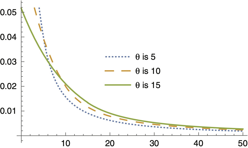
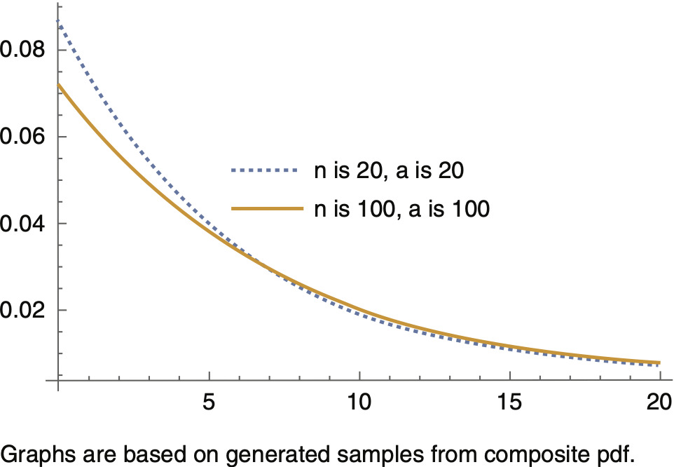
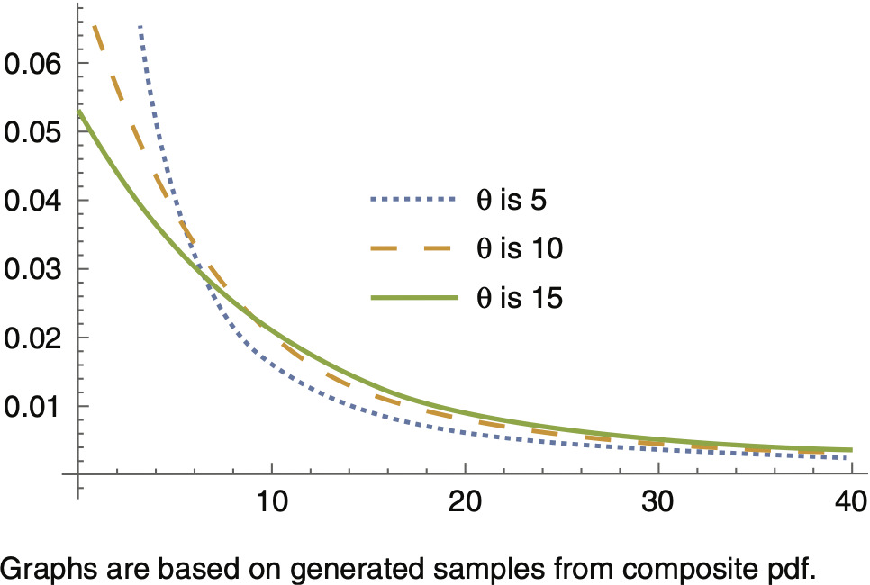
Figures 4.1 through 4.3 provide graphs of the predictive density for different values of θ and a, revealing that as n increases, the tail of the predictive density becomes heavier, and as a result, at a specific level, say 0.99, VaR increases. Simulation studies confirm this conclusion. Figure 4.3 is a graph of the predictive density for fixed values n = 50, a = 50, and for three different values of θ based on which samples from the composite pdf are generated. Similar to what is shown in Figure 1.1, as θ increases, the tail of the predictive density becomes heavier, causing VaR at a specific level, say 0.99, to increase.

Figure 4.1.Predictive density for selected values of n and a, 5

Figure 4.2.Predictive density for selected values of n and a, 10

Figure 4.3.Predictive density with various values, n 50 and a 50

5. Numerical example

The data set in Table 5.1 is a random sample of size 200 generated from the exponential-Pareto composite pdf (1.1) with parameter θ = 5. For this data set, the value of m is 86. The Bayes estimate is 4.9878, and the MLE is 4.935488. Simulation studies indicate that the Bayes estimator is more accurate than the MLE. Due to the long-tailed composite distribution, based on a sample of size n = 200, nine intervals of unequal widths are used to assess the goodness of fit of the data via a chi-square test. The observed and expected frequencies for the proportion of observations within each class-interval are given in Table 5.1.

In Table 5.2, $p_k$ denotes the observed percentage of observations in the class-interval $k, k=1,2, \ldots, 9$. $e_k$ denotes the expected proportion of observations in the class-interval $k$. Note that to get $e_k$, a Bayes estimate of 4.98786 for $\theta$ is used in the cdf of the composite distribution. At the 0.05 level of significance with 7 degrees of freedom, the critical value for the chi-square test is 14.067 . As a result, there is not enough evidence to reject the null hypothesis that $\hat{\theta}_{\text {Bayes }}=5$.

6. Conclusion

A Bayes estimator via inverse gamma prior for the boundary parameter θ, which separates large losses from small losses in insurance data, is derived based on the exponential-Pareto composite model. A Bayesian predictive density is derived via the posterior pdf for θ. The “best” value for a is selected through an upper limit (a decreasing function of n) on the variance of the inverse gamma prior distribution. Simulation studies indicate that even for a large sample size, the Bayes estimate outperforms MLE if the “best” values of hyperparameters a and b are used in computations. Having values for the hyperparameters, the predictive density is used along with a numerical method in Mathematica to compute VaR at the 70% level.