Strategies for Modeling Loss Development: Curve Fitting, Credibility, and Layer Adjustments

undefined

1. Introduction

Because of the delay from the date an event occurs until it is reported and ultimately paid, insurance companies, unlike other businesses, do not know whether their products are being adequately charged for or whether they were sold at a profit or at a loss. Actuaries rely on loss development patterns to help estimate all of this.

The problem with loss development data is that it contains summarized information consisting of the payments of different types of claims as well as reserve setups, increases and takedowns for reported data. This makes it difficult to fit a loss development pattern to a simple model that can be used to reduce the number of parameters, perform credibility weighting, apply adjustments for different layers, or other tasks.

This paper discusses some strategies to better handle the modeling of loss development patterns. Specifically, the following is discussed:

1. Some improved curve- and distribution-fitting methods.

2. Credibility-weighting techniques for fitted curves and distributions.

3. Methods for modeling across continuous variables.

4. Determination of the optimal look-back period for pattern selection.

5. Calculation of the error distribution for both the process and parameter variance.

6. Formulas for converting and modeling across different loss caps, retentions, and policy limits.

All of the models in this paper can be implemented as full Bayesian models solved using Markov chain Monte Carlo, or more simply in spreadsheets. This allows for easier adoption. It also facilitates implementation in account rating engines where credibility weighting can be performed on an account’s individual loss development pattern. Both versions will be discussed. Throughout this paper, unless otherwise mentioned, all modeling is performed on the age-to-age factors and all references to LDFs refer to these.

1.1. Outline

The next section discusses two strategies for smoothing development patterns. The first involves fitting a curve and the second involves fitting a distribution. Section three then discusses a method to perform credibility weighting on these models. The related topic of modeling on continuous variables is handled as well. Section four discusses the topic of choosing the optimal look-back period and section five elaborates on the estimation of the error distribution. The final section, section six, discusses applying layer adjustments to loss development factors.

2. Fitting curves and distributions to loss development patterns

Selecting individual loss development factors without paying attention to the shape of the curve discards a large amount of useful information about the relationship between the LDFs that can be used to improve the accuracy of selections. As mentioned in England and Verrall (2002) and others, selecting parameters for every single age is over-parameterized, meaning that more parameters are being chosen than necessary, which will increase the prediction variance. Some curve-fitting strategies for LDFs are discussed in this section that improve upon the inverse power curve (Sherman 1984) and fitting a distribution to the development pattern (Clark 2003).

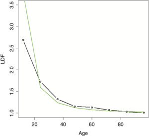
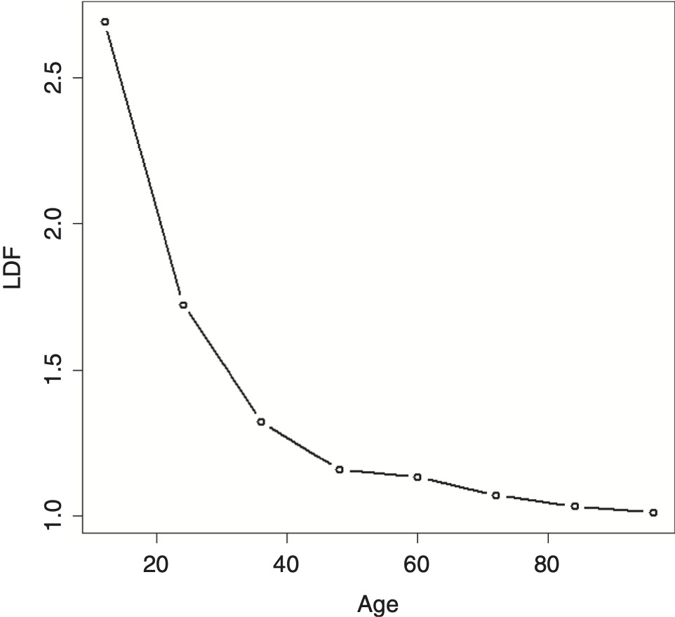
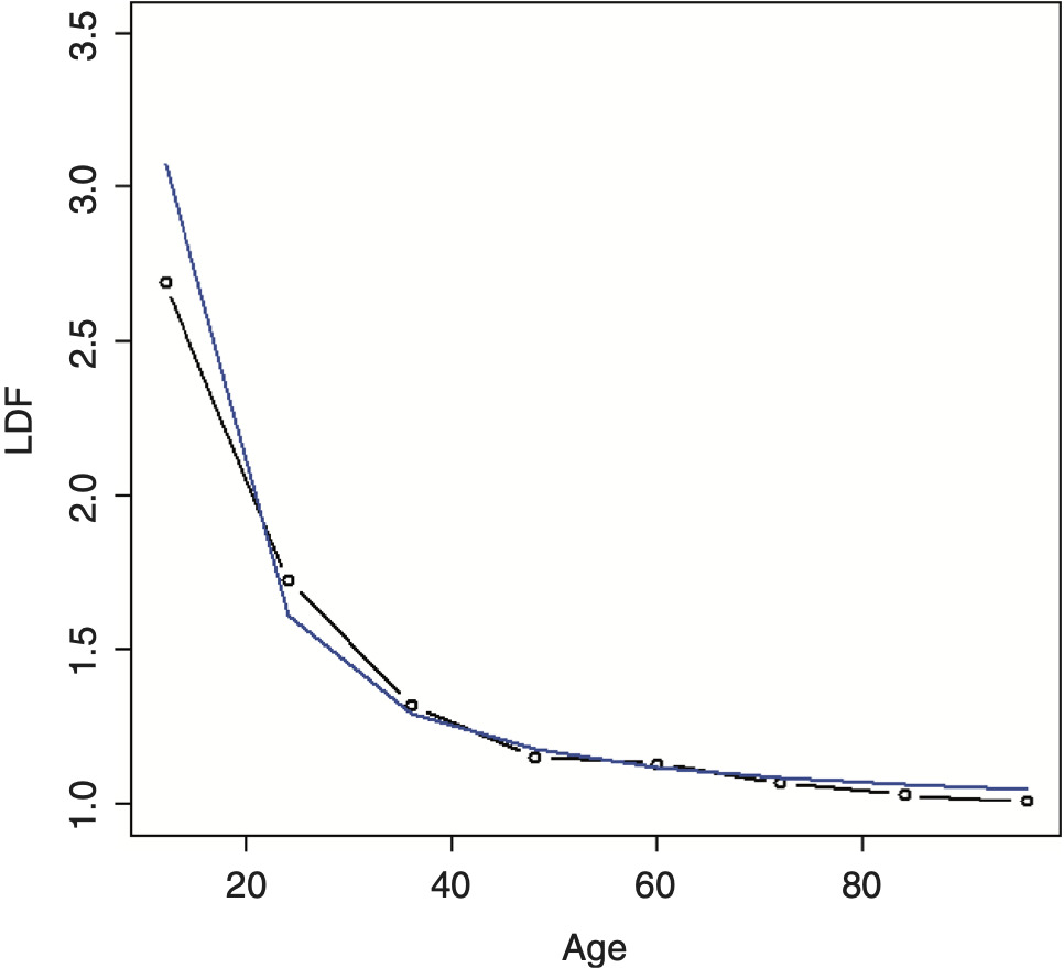
The example data shown in Table 1 will be used to illustrate many of the methods in this paper. The resulting average LDFs are shown in Figure 1.

2.1. The inverse power curve

The inverse power curve (IPOC) is a well-known method used to help smooth LDFs (Sherman 1984). This curve can be fit by using the regression equation, as mentioned in the paper^[1] (ignoring the c parameter and setting it equal to zero):

$$\log (L D F-1)=A+B \times \log (t), \tag{2.1}$$

where A and B are regression coefficients and t is the age. In the author’s experience, it can be a useful tool to help smooth out some LDFs, especially in the latter portion of the curve, although it often has trouble fitting the entire curve. This depends on the book of business, however. Also, solving this regression equation using ordinary regression gives too much weight to the tail portion of the curve, as mentioned in Lowe and Mohrman (1985). This is not an issue if using an extrapolation from earlier, more stable points to predict later ages in the curve, as is commonly done, but can be an issue when attempting to fit to the entire curve. Several improvements to this curve will be discussed in the following sections.

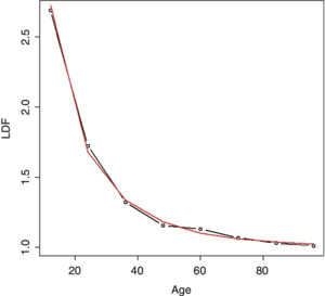
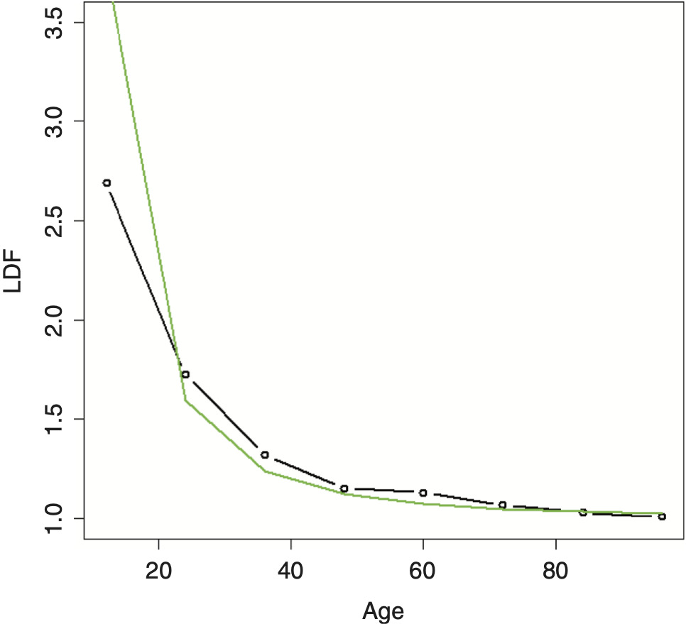
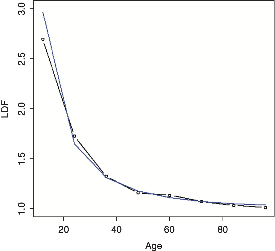
Fitting the IPOC on the example data produces the result shown in Figure 2. As can be seen, it does a relatively poor job of fitting to the data.

2.2. An improvement: The DIPOC

One way to improve the fit of the IPOC is by addressing the issue raised in Lowe and Mohrman (1985) regarding the weights. Instead of using ordinary regression to solve for the parameters, another type of regression can be used. The method described here can be implemented either on the individual LDFs of a triangle or on the average LDFs by age.

An assumption that will be used is that the variance of an LDF is inversely proportional to the sum of losses in the previous period, and so the variance of a weighted average LDF is proportional to the total sum of losses in the previous period. (So, for example, the variance of the first LDF is related to the losses from the first age.) This should be the case since the variance of the losses for a subsequent age for two equally sized and uncorrelated accounts is equal to twice the variance of one of these accounts. To convert these losses into LDFs, they are divided by the sum of the losses in the previous age; and so the variance is divided by the square of this sum (since it is not a random variable). Thus, the denominator of the LDF variance for both equally sized accounts combined will be two squared greater than that of a single account. And so the variance of the combined LDF will be 2/2² or half of that of each of the accounts separately; assuming any other relationship between variance and losses in this simple example will not agree with this result and will lead to inconsistencies.

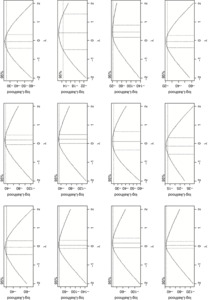
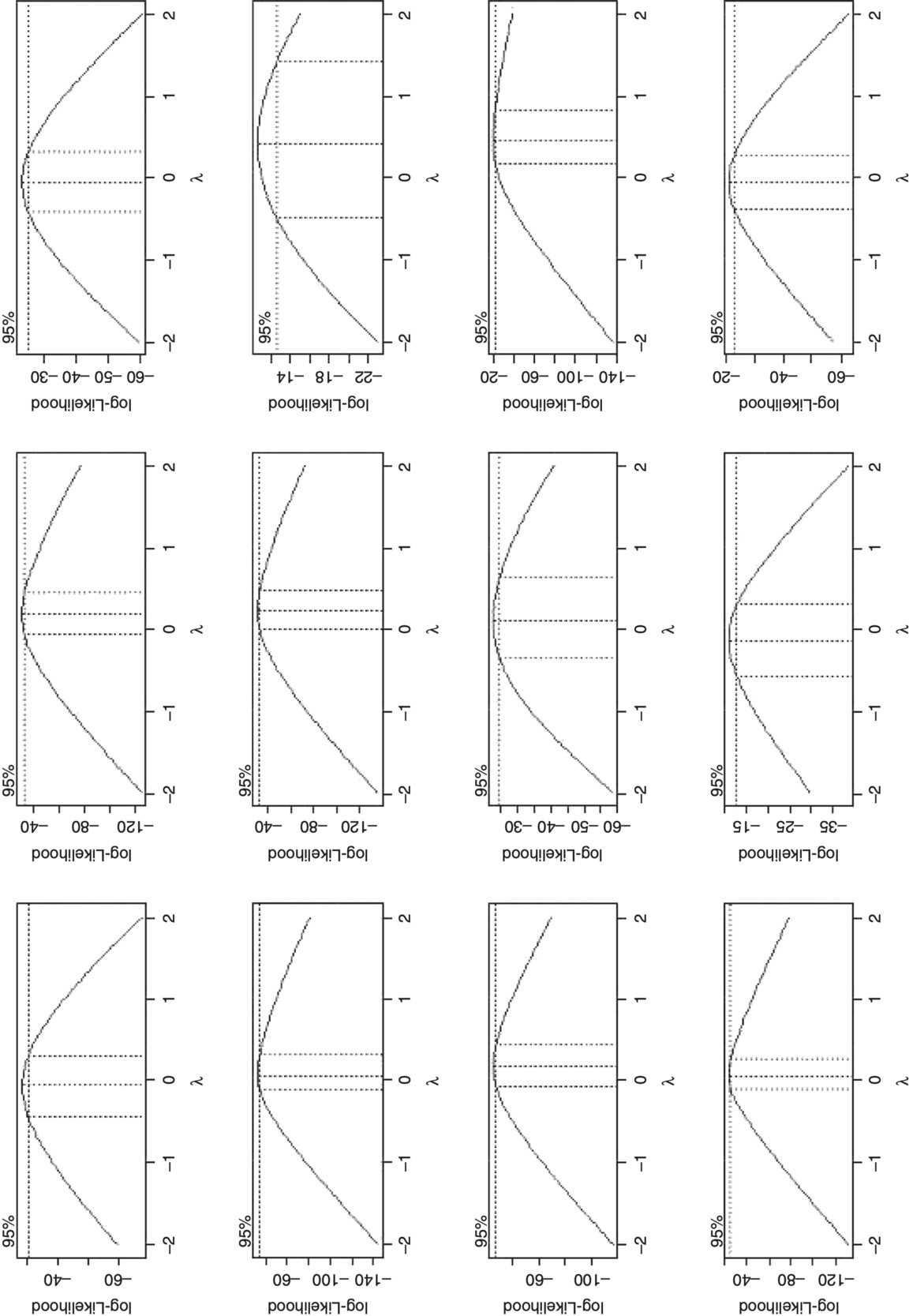
Turning back to the regression, an important question to ask is what is the most appropriate distribution family for loss development factors. If the errors are assumed to be additive, a normal distribution family should be used. If instead errors are assumed to be multiplicative, a gamma distribution family should be used, since this will make the standard deviation proportional to the mean. If the error distribution is between additive and multiplicative, a Tweedie distribution family should be used. To help answer this question, a Box-Cox test was run on actual data from various commercial lines of business using the MASS package in R (Venables and Ripley 2002). This tests for the amount of skewness by determining the correction required in order to make data approximately normally distributed. The transformation has the following forms: (x^λ − 1)/λ for λ not equal to zero; and log(x) for λ equal to zero, where x represents the values in the data and λ is the transformation parameter, which can be solved for using maximum likelihood. A resulting value of one provides no meaningful transformation and indicates that the data is already approximately normally distributed; a value of zero or close to zero indicates that the data is closer to being lognormally distributed and that the gamma distribution family would be ideal in the regression context; and a value in between zero and one indicates that a Tweedie would be best. The test results in Figure 3 show the 95 percent confidence interval and was conducted using internal company data on the LDFs minus one for various ages (going across) for various commercial lines of business (going down) for both primary and excess as well as both occurrence and claims made business. As can be seen, it produced results mostly around zero, thus showing that the gamma distribution family, though not 100 percent perfect, is suitable for modeling LDFs.

Using a gamma distribution family assumes that the standard deviations of the LDFs minus one are proportional to the mean, or in other words, that the coefficients of variation (CoV, the mean divided by the standard deviation), are constant. In practice, the CoV should also vary with the age of the triangle, as LDFs tend to be more volatile at the very early ages where the loss volume is low, as well as at the later ages where the volatility can be very high relative to the low expected amounts of development. To model this relationship, a curve will be used to determine a CoV factor by age. The CoV for each age is equal to this CoV factor divided by the square root of the loss volume, which agrees with the relationship mentioned that the variance of an LDF is inversely proportional to the loss volume. This CoV factor curve should be increasing (faster than the losses, that is), which allows for the later LDFs to be more volatile. Having the CoV be related to the losses also allows for the earlier ages to have more volatility since the loss volume is lower thus making the CoV higher.

To summarize, where A, B, I, and J are all parameters solved via maximum likelihood, the steps are as follows (note that what we refer to as beta, Excel refers to as the inverse of beta.):

$$\text {Fitted} \mathrm{LDF}_{\mathrm{i}}=\exp \left(\mathrm{A}+\mathrm{B} \times \log \left(\text {age}_{\mathrm{i}}\right)\right)+1$$

$$\text {CoV Factor}_{\mathrm{i}}=\exp \left(\mathrm{I}+\mathrm{J} \times \text {age}_{\mathrm{i}}\right)$$

$$\operatorname{CoV}_{\mathrm{i}}=\operatorname{CoV}_{\mathrm{i}} \text {Factor}_{\mathrm{i}} / \sqrt{} \operatorname{Loss}_{\mathrm{i}}$$

$$\alpha_{i}=1 / \operatorname{CoV}_{\mathrm{i}}^{2}$$

$$\beta_{\mathrm{i}}=\alpha_{\mathrm{i}} /\left(\text {Fitted} \mathrm{LDF}_{i}-1\right)$$

$$\operatorname{loglik}=\sum \log \left(\operatorname{Gamma} \operatorname{PDF}\left(\begin{array}{c} \text {Actual} \mathrm{LDF}_{\mathrm{i}} \\ -1, \alpha_{\mathrm{i}}, \beta_{\mathrm{i}} \end{array}\right)\right).$$

What was done here is similar to a double GLM that can be implemented in a spreadsheet environment. (Note that the equation for the CoV is slightly different from the inverse power curve equation.)

As mentioned, the actual LDFs used can either be the average LDFs across all selected years, in which case the losses used should be the sum of the losses across these years used for calculating the LDFs, or they can be the individual LDFs of the triangle. If the CoV parameters are the same, the two approaches will yield identical results, as can be confirmed. This method usually works well on either, although modeling on the individual LDFs should produce more robust estimates of the variance parameters, which may make the fit more accurate. If the variance parameters are also being used to estimate the variability in the LDFs, then using the individual LDFs is definitely preferred.

If this method is run on the individual LDFs, it will fail if any of the loss volumes are zero, which can occur at early ages of a triangle, since these LDFs are infinite. One solution is to set all zeros in the triangle to a very small positive value. Another solution is to use the overall average for these early ages.

LDFs equal to one should be set to a very small value above one, since the gamma distribution is not defined at zero. This method will similarly fail with LDFs less than one, which can be frequent in reported loss triangles. A simple solution is to exclude all LDFs less than one when running the initial model. Then, a bias correction can be calculated by calculating the difference between the average empirical LDFs with and without these negative development LDFs, and then fitting a curve through these differences to smooth them out. (A spline curve can be used, which is described in the next section.)

Another alternative is to subtract a number slightly less than one from the LDFs instead of subtracting one when calculating the gamma likelihood, such as 0.9 or 0.8. This will allow the likelihood of more of these negative development LDFs to be included. A revised CoV factor needs to be calculated so that the variance of each LDF is as expected. This can be done using the following formula, where Base is the number subtracted from the LDFs:

$$\text{Adjusted CoV Factor} =\frac{\text {CoV Factor} \times(\text{Fitted LDF}-1)}{\text{Fitted LDF}-\text {Base}} . \tag{2.2}$$

The lower the base used, the more LDFs that can be included, but the more distortion to the model, since the LDFs minus one were assumed to be gamma distributed. Different bases should be tested to make sure that the method is not too sensitive to the choice of a base. Testing this approach on actual data had mixed results, however. With this method, the expected LDFs are still required to be greater than one.

As a final note, this curve, as well as the method described in the next section, generally works better with quarterly evaluations, although this is not essential and depends on the length of the development period for the line. Quarterly evaluations increase the number of data points, which makes it easier to both fit and evaluate the curve.

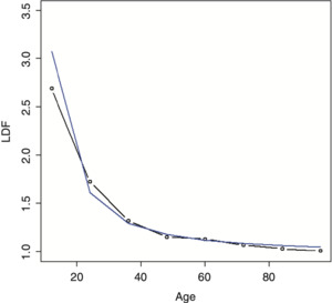
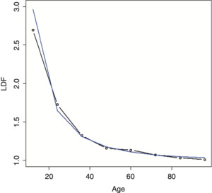
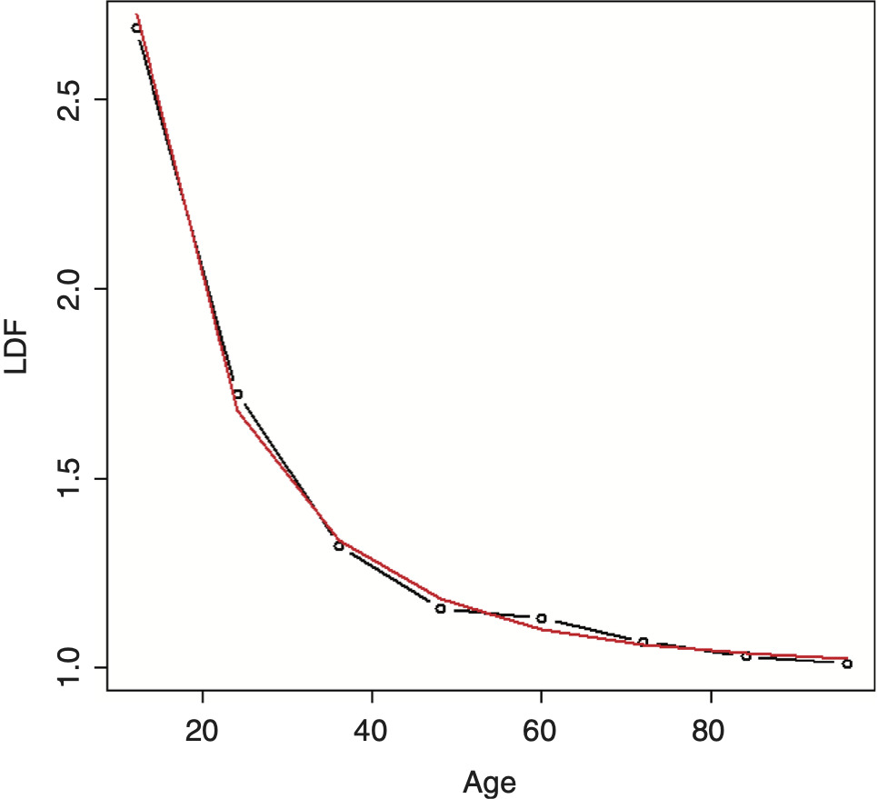
Running this double inverse power curve (DIPOC) on the example data yields the result shown in Figure 4. The fit is improved, but is still not great.

In the author’s experience of using this method on actual data, the DIPOC can perform well on some lines, but less well on others. For these cases, the method from the next section should be used.

2.3. Adding smoothing: The SMIPOC

The following model can be described as a combination of the inverse power curve and the generalized additive model suggested by England and Verrall (2001) that they use to model the incremental paid or reported loss amounts. Here, however, we will be modeling on the actual LDFs instead, as we have been doing, because it is easier to implement, produces results that are more consistent with traditional actuarial practice, and works better with credibility weighting (as is shown later). It also involves solving for fewer parameters so that it can be implemented in spreadsheets.

Before we begin explaining how this model works, we will briefly explain splines and additive models. An ordinary regression model has a dependent variable that is a linear function of one or more predictive variables and has the form

$$Y_{i}=\sum_{j} B_{j} X_{i j}.$$

An additive model, instead of just linear functions, allows for any function, and has the form

$$Y_{i}=\sum_{j} f\left(X_{i j}\right).$$

Usually, some type of smoothing function is used that helps adapt the curve to the actual data, even if the relationship is not perfectly linear. Cubic splines are a very common choice since they do a good job of adapting the curve to the data and results in nice, smooth curves.

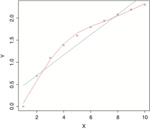
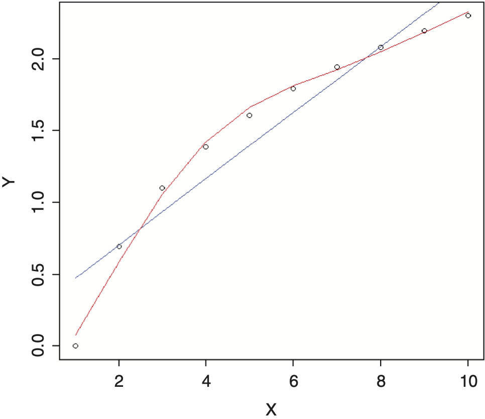
For example, if we were trying to fit a regression model to the data below and were not able to find a simple transformation of the independent variable that nicely fit the data, such as a logarithm, we might consider using an additive model. The results, using a linear regression model (blue line) versus an additive model (red line), are shown in Figure 5. Note how the additive model nicely adapts the shape of the curve to the data.

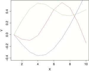
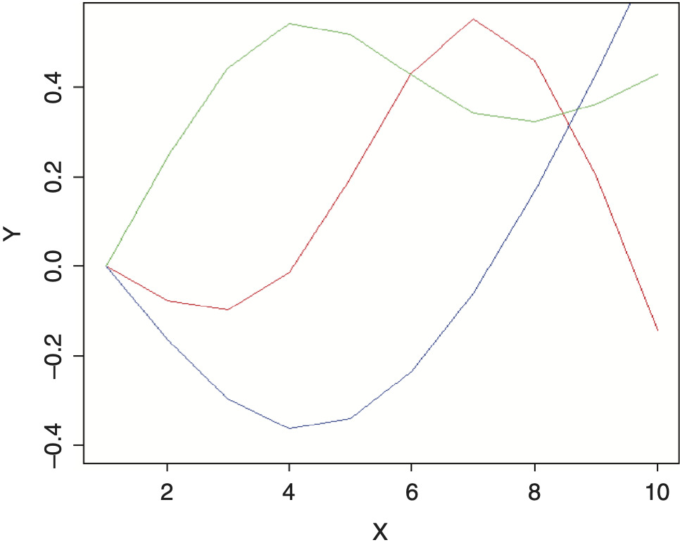
An additive model can also be implemented with an ordinary regression model using splines.^[2] These are functions that generate multiple new numeric sequences based off of the original sequence that can be used for smoothing. These new variables can then be plugged into a standard regression model with the same result as an additive model. The example shown above used three natural cubic spline transformations off of the numeric sequence from one to ten and are graphed in Figure 6. Each of these resulting curves represents one of the degrees of freedom of the spline. By multiplying each curve by a coefficient and adding the results together, smooth curves can be fit to data of multiple forms and shapes. The benefits of this approach are that splines work better for the credibility procedure that will be presented and allow additive models to be implemented from within spreadsheets.^[3] A full discussion of additive models is outside of the scope of this paper.

Having described the benefits of additive models and how they work, it becomes clear why we would want to use them in a loss development model; it is often difficult to find a simple parametric shape that fits nicely to the entire curve. Additive models solve this problem by adapting the curve to the data. A downside, however, is that they can sometimes over-fit.

This method works best when the spline is generated on the logarithm of age, and so is very similar to the inverse power curve, but with additional smoothing to help fit the data better. This model will be referred to as the smoothed (double) inverse power curve, or SMIPOC.

Compared to the DIPOC, the spline/additive model often provides a much better fit to the data. The regression equation used here is

$$\log (L D F-1)=A+B \times s(\log (t)).$$

Where A and B are the regression coefficients, t is the age, and s is a smoothing cubic spline function. Using splines, this can be extended to the following (assuming that a spline with two degrees of freedom was used):

$$\log (L D F-1)=A+B t^{(1)}+C t^{(2)}, \tag{2.3}$$

where A is the intercept of the curve, and B and C are the slope parameters for each of the generated spline variables, t⁽¹⁾ and t⁽²⁾, on the logarithm of the age. (Superscripts were used to denote the different spline variables.) The parameters should be solved for the same way as described for the DIPOC.

The number of degrees of freedom to use for the spline depends on the data. Often using a spline with two degrees of freedom produces a good fit, but another degree of freedom can be added if necessary. A likelihood ratio test can be performed to see if additional parameters are warranted as well as to compare this model to the DIPOC. The significance level for this test is equal to one minus the chi-square cumulative distribution function at twice the difference in the likelihood, with the degrees of freedom equal to the difference in the number of parameters between the models being tested. So, for example, to test if this model is superior to the DIPOC, assuming that a spline with two degrees of freedom was used, the degrees of freedom parameter should be set to one, since this SMIPOC has one additional parameter.

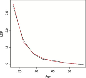
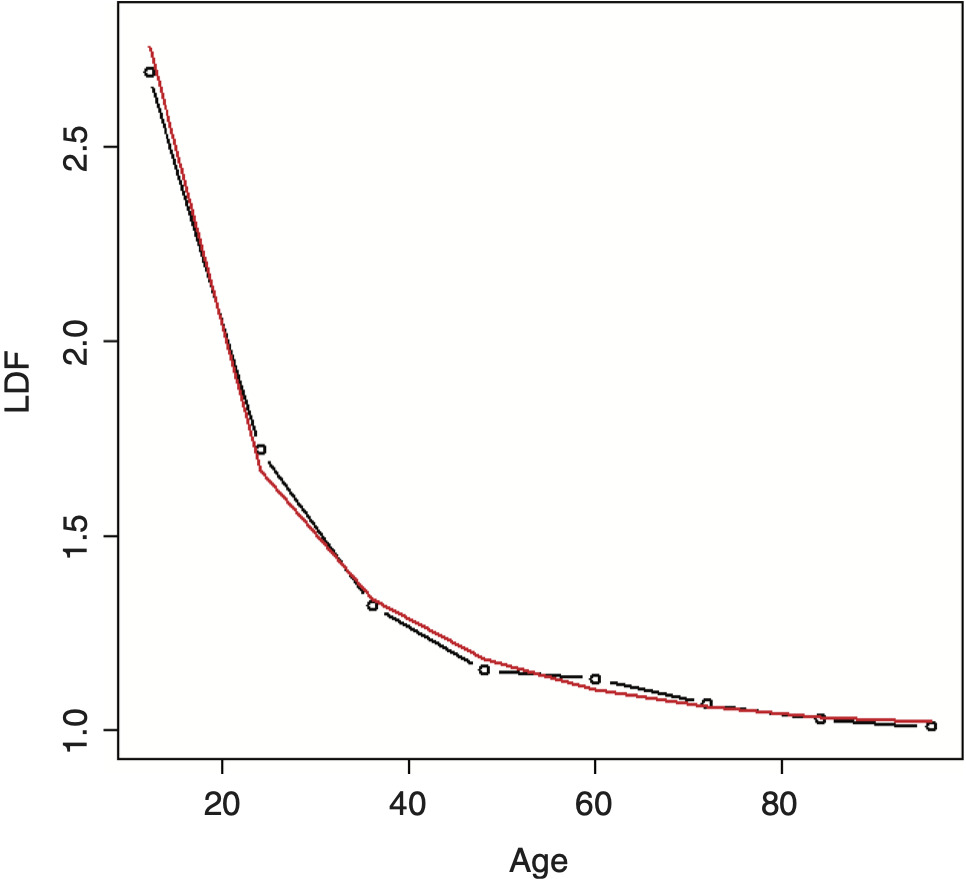
Running this model on the example data produces a much better fit, as can be seen in Figure 7. A chi-square test to see if this model is preferred over the DIPOC produces a value of 0.4 percent, which is very significant.

2.4. Fitting a right truncated distribution: The RIPOD and SMIPOD

Clark (2003) fits a distribution to the completed percentages as an alternative strategy for modeling a loss development pattern. Taking this approach of fitting a distribution, a different method for performing this task will be suggested here that is based off of the procedure described in Korn (2016) and used to model claim reporting and payment lag times.

When fitting distributions, for example, left truncation is present if a policy has a retention, since both the amounts and the number of claims below the retention are unknown. When looking at reporting lags, for example, right truncation is present, since nothing is known about the number and times of the claims that will arrive after the evaluation date. To control for left truncation with MLE, the likelihood is divided by the survival value at the retention; similarly, to control for right truncation, the likelihood should be divided by the cumulative distribution function (CDF) at the truncation point. (If both left and right truncation are present, as can be the case, as shown shortly, the likelihood should be divided by the difference of the CDF values at the two truncation points.)

This will be used to model the timing of each dollar (or euro, etc.) in a development triangle. Right truncation is present since nothing is known about the number of dollars that will be paid (or reported) or the timing of these payments after the evaluation date. Note that modeling the times of the individual payment dollars directly assumes that the payment of each dollar is independent, which is clearly not the case, but with enough payments, this is immaterial. To apply this method to a paid triangle with yearly evaluations for year 2015 at 24 months and an evaluation date of 12/31/2017, for example, the log-likelihood of each dollar is equal to $\log \left(\frac{C D F(24)-C D F(12)}{C D F(36)}\right)$. The difference of the CDFs was used in the numerator since all of these dollars were paid between 12 and 24 months from the beginning of the year. The total log-likelihood for this year/evaluation period is equal to the product of this log-likelihood and the (incremental) number of dollars paid at this period. If any year is used starting from some point other than the beginning, which occurs if the n most recent calendar years are used, the normal rules of MLE should be applied, namely, the left truncation of the starting point should be reflected; this would change the denominator to be the difference between the CDFs at the right truncation point and at the starting point. Note that this method can be performed even if the losses are negative, i.e., some LDFs are less than one, although the expected development is still expected to be positive. Once a distribution is fit to the loss development data, age-to-ultimate factors can be calculated by taking the inverse of the fitted CDF values. Age-to-age factors can be obtained by dividing consecutive age-to-ultimate factors.

Since only CDF/survival values are needed for this to work, there is some flexibility in the type of distribution that can be used; a curve can be fit to the survival values without having to worry what the corresponding probability density function is. One such curve that works well (based on the author’s experience) is to use the inverse power curve equation, but with a logit transform instead of a log (and also do not subtract one from the value as done with LDFs). So, the equation for this curve is

$$s(\text {age})=\operatorname{ilogit}(A+B \times \log (\text {age})), \tag{2.4}$$

where s(x) is the survival function at x and ilogit is the inverse of the logit function. This function ensures that the resulting survival values are between zero and one. It will not ensure, however, that the values will be strictly decreasing, which would result in negative likelihoods, but this will usually be the case anyway.

Using this curve, the resulting distribution turns out to be identical to using the log-logistic distribution, which is one of the recommended distributions mentioned by Clark (2003). Since this equation is based on the inverse power curve, it will be referred to as a right-truncated inverse power distribution (RIPOD), since it is a distribution and not just a curve, keeping with the nomenclature of this paper. Fitting the RIPOD on the example data produces the result shown in Figure 8.

It can be seen that this fit is not far off but is still imperfect. When this is the case, additional smoothing can be added via a spline, similar to what was done for the inverse power curve. This smoothed inverse power distribution (SMIPOD) often performs better, although its performance can be compared to the RIPOD using a likelihood ratio test. There is less guarantee that this curve will be strictly decreasing, but most of the time it is. (If necessary, it is possible to constrain the survival values when performing the fit to be strictly decreasing.) It also usually produces a lower estimate of the tail, which is a potential issue mentioned by Clark (2003) with the log-logistic distribution. The fitted tail was 1.171 for the RIPOD while it was 1.060 for the SMIPOD, which seems much more reasonable, given the data. Fitting this distribution on the example data produces the result shown in Figure 9. A likelihood ratio test to see if the SMIPOD is preferred over the RIPOD produces a value of 9.2 percent, which is borderline significant—although, based off of the graphs and the resulting tail values, the SMIPOD would probably be preferred.

When performing MLE to fit the SMIPOD on actual data, it is sometimes difficult for the maximization routine to arrive at the global maximum. Appropriate starting values should be chosen, which is always the case, but even more so with this method. One method of selecting good starting values is to set the initial SMIPOD parameters to those values that produce the same results as the RIPOD. This way, the likelihood of the RIPOD can only be improved. To do this, another optimization routine can be run that minimizes the squared or absolute differences between the CDFs of the two methods before running the actual SMIPOD optimization. This should work well with a spline having two degrees of freedom. In the author’s experience, using this method with a spline having three degrees of freedom was unstable and produced unsatisfactory results. Dividing the SMIPOD equation by the survival value at a low value close to zero can also help add stability to this distribution. Another possible solution is to optimize the inverted survival function parameters, as is explained in the next section. If this is done, the final survival function parameters should be constrained so that they are decreasing because otherwise negative likelihoods would result, which would cause an error in the routine.

3. Credibility weighting

3.1. Method of credibility weighting

Bayesian credibility is used as the credibility weighting method throughout this paper. This method can be implemented without the use of specialized Bayesian software: The prior distribution (that is, the distribution of the hypothetical means for each group, in Bayesian terms) that will be used for these models is the normal distribution, which is the most common assumption. Since the distribution of maximum likelihood parameters is assumed to be approximately normal, this is a conjugate prior and the resulting posterior distribution (the credibility-weighted result) is normal as well. Using MLE returns the mode of a distribution, which will also be equal to the mean for the normal distribution, and so will return identical results to that produced using specialized Bayesian software. Further implementation details are discussed in the following section.

3.2. Applying credibility to a curve

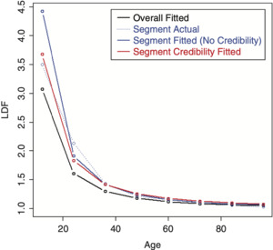
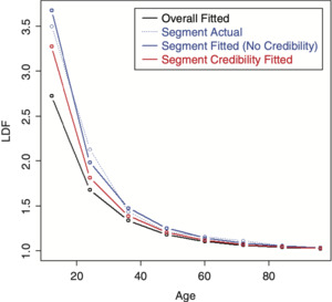
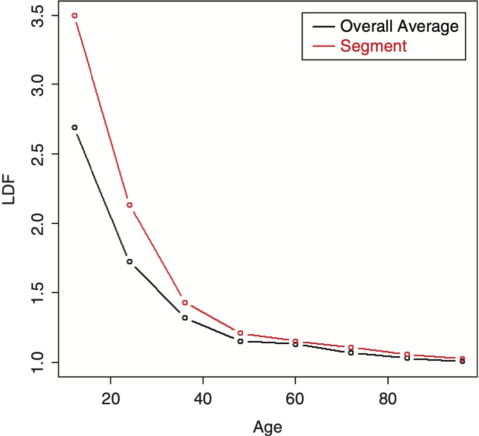
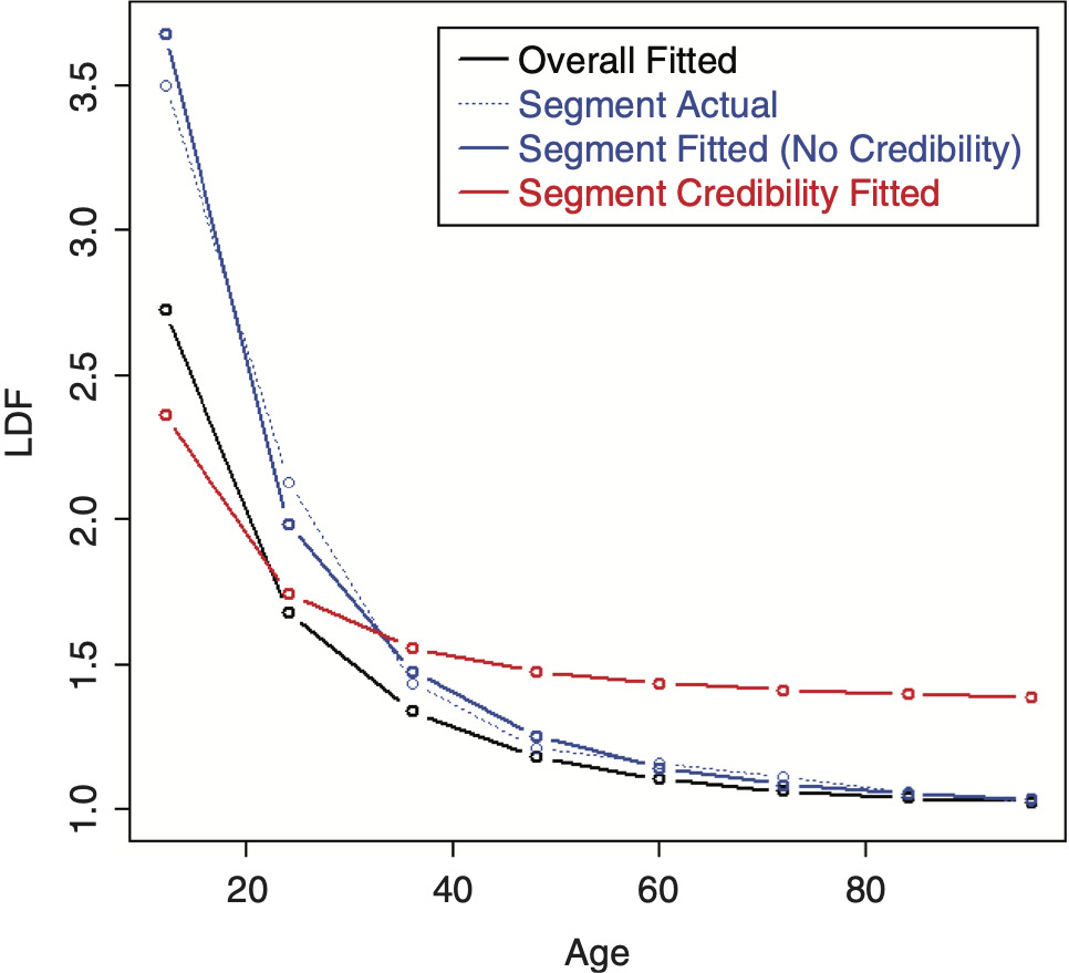
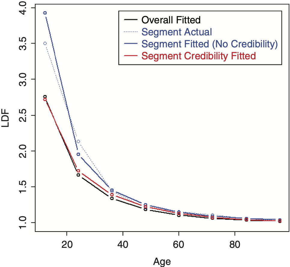
To perform credibility weighting across different segments using Bayesian credibility, Bayes’ formula would be used: f(Parameters|Data) ∼ f(Data|Parameters) × f(Parameters), or equivalently, Posterior(Parameters, Data) ∼ Likelihood(Data, Parameters) × Prior(Parameters), and the regression parameters would be used for calculating this prior likelihood component, which is the credibility component of the likelihood. However, doing so often results in credibility-weighted curves that do not lie in between the complement curve, and the curve that would result if no credibility were performed. This is a nonintuitive result that is difficult to understand and to justify. An example segment that will be used for illustration is shown in Table 2 (using the same overall triangle shown in Table 1). A comparison between the average LDFs of the segment versus the overall is shown in Figure 10. Performing this naive credibility technique with the SMIPOC on the example data is shown in Figure 11. It produces curves that intuitively seem wrong. This is especially true for spline curves, since the spline coefficients are highly dependent on each other and applying separate prior/credibility penalties on each coefficient leads to odd results. The same is true for the DIPOC, although to a lesser extent. This curve is shown in Figure 12. It is much better behaved than the SMIPOC but still produces a nonintuitive result, as can be seen from the fact that the credibility-weighted curve crosses over the independently fitted curve.^[4]

To fix this issue, the curve can be reparameterized. The first step is to invert the regression equation (2.1 or 2.3) to solve for the LDFs. Doing so results in the following equations for the IPOC/DIPOC. Since there are two parameters, two LDFs are needed at two separate ages to solve for them:

$$B=\frac{L_{1}-L_{2}}{\log \left(\frac{t_{1}}{t_{2}}\right)}. \tag{3.1}$$

$$A=L_{1}-B \log \left(t_{1}\right), \tag{3.2}$$

where L = log(LDF − 1) at two different ages along the curve.

Now, given any two LDFs of the fitted curve, the original regression parameters can be solved for. And given these, all of the LDFs of the curve can be calculated. Ignoring the middle step, the entire curve can be constructed from these two LDFs. Since the entire curve can be defined by these two LDFs, they can also be considered as the parameters of the curve. This being the case, the prior likelihood (the credibility component of the likelihood) can be calculated using these new parameters instead.^[5] Instead of using the actual LDFs, it’s recommended to use the logarithm of the LDF minus one so that the relationships between different segments’ LDFs will be multiplicative. The ages for these LDF parameters can be selected as being equally spaced along the ages used to perform the fit, but they can be tweaked if needed. Note that even though the credibility weighting is being performed on only two LDFs of the curve, the entire curve is still being credibility weighted, since changing these LDF parameters affects the entire curve as they are the new curve parameters. The same applies to the SMIPOC, except that three or four LDFs should be used, since this curve has three or four parameters that are being credibility weighted.

It is probably best to invert the equations when implementing a full Bayesian model. For an MLE model, this is not necessary, however (unless implementing a multidimensional model or modeling across continuous variables, which is discussed later), since any fitted LDFs along the curve can be calculated using the curve parameters and thus can be used to calculate the prior likelihood component, effectively “pretending” that the equation has been inverted and reparameterized. Doing this will yield the exact same results as if the inversion had actually been performed. The same applies to a right-truncated fitted distribution except that the logit of the survival values should be used as the new parameters instead.

For the MLE model, the complement of credibility for each parameter can be taken from the results from fitting a curve to all segments combined, and not the actual empirical LDFs, since these are subject to more volatility. Or, alternatively, if all of the segments’ likelihoods are maximized together, the complements can be determined from the model and set as parameters. For a Bayesian model, the latter is usually performed, but this may be too many parameters to solve for simultaneously with an MLE model. However, using the curve resulting from combining all segments may be easier to explain and justify to a less technical audience. To summarize, to perform credibility weighting, the following component is added to the log-likelihood:

$$\sum_{\substack{c=\text {Ages Used} \\ \text {For Credibility} \\ \text {Weighting}}} N\left(\begin{array}{c} \text {Fitted} L_{C}, \text {Complement} L_{C} \\ \text {Between Variance} \end{array}\right), \tag{3.3}$$

where L = log(LDF − 1) and N(A, B, C) is the logarithm of the probability density function (PDF) of a normal distribution at A, with mean and variance of B and C, respectively. The fitted LDFs are determined from the appropriate curve equation (2.1 or 2.3). There should be only one set of parameters for calculating the CoV factors that is shared across all segments, unless a strong reason exists for doing otherwise. This is straightforward if all of the segments are being run together. If not, the CoV parameters can be taken from the curve fit to the combined data. The equations for inverting the SMIPOC are shown in Appendix A for both three and four parameter curves.

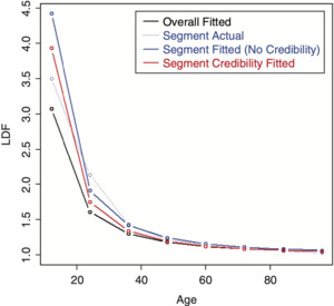
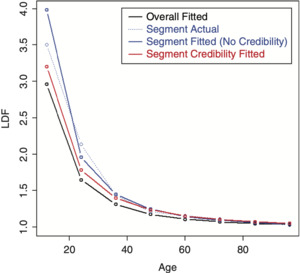
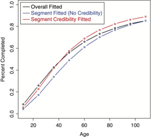
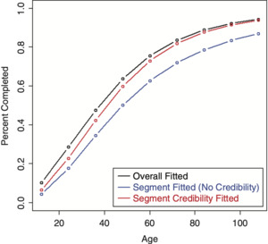
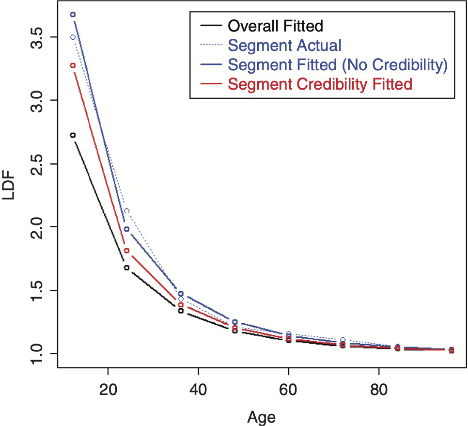
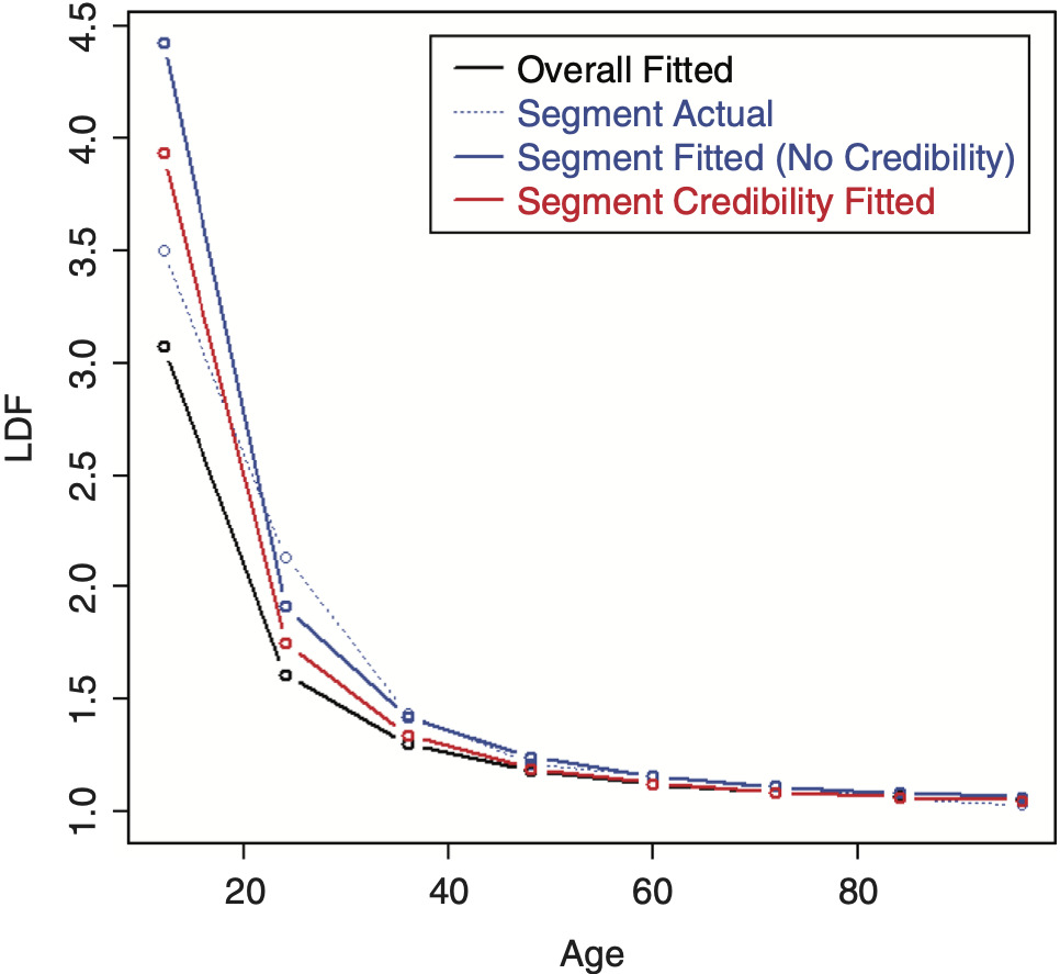
Performing credibility weighting on the example data using this method with a three parameter SMIPOC is shown in Figure 13 and with a DIPOC in Figure 14.^[6] These results are much more in line with our intuitive expectations of where credibility-weighted curves should end up. (Although there is still no guarantee that the resulting age-to-ultimate factors will do the same, they usually do.)

In this example, note that even though the credibility-weighted curves lie in between the complement and the independently fitted curves, this may not always be the case. Sometimes tweaking the ages used for the LDF parameters can fix this issue. If not, and assuming that this is a desired property, the prior/credibility component of the likelihood can be calculated at every single age but assigned weights equal to the ratio of the number of curve parameters divided by the number of ages so that the overall effect of the prior is mostly unchanged. Doing this probably has little theoretical justification but can still be a useful, practical method.

3.3. Applying credibility to a distribution

The same applies to a distribution fit to the loss development pattern. Applying credibility to the original parameters may result in poorly behaved results. Using the inversion method, credibility can be applied to the (logit) survival values. Using the survival values will help the age-to-ultimate factors be better behaved, which may be more important than the age-to-age factors. The inverted formulas for the distributions are the same as those for the curves, except that the logit of the survival values are substituted for the logarithm of the LDFs minus one.

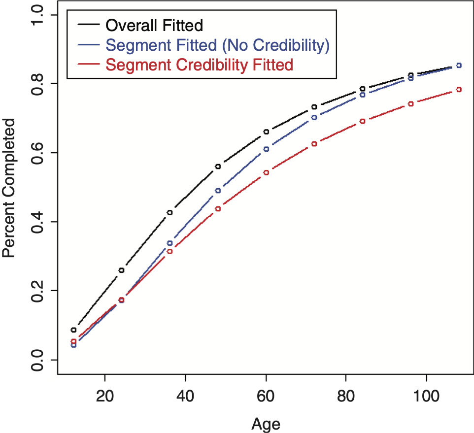
The LDF and CDF results from fitting a RIPOD by performing credibility on the original parameters are shown in Figures 15 and 16, respectively.^[7] It can be seen that the credibility-weighted LDFs cross over the independently fitted curve towards the end. For the CDF, a revised tail estimate causes the credibility-weighted curve to lie above both the complement and the independently fitted curve.

Inverting the parameters for the RIPOD helps the performance, but is still not great.^[8] Figure 17 shows the LDFs, which look as expected. The CDF, however, shows a non-intuitive result due to a revised tail estimate and is shown in Figure 18. This result seems to be due to the rigidity of the curve; adjusting some of the earlier factors causes the curve to increase past the complement.

The SMIPOD performs better because it is a more flexible curve. Figures 19 and 20 show the resulting LDFs and CDF preforming credibility on the original parameters.^[9] In this case, the credibility-weighted curves are performing satisfactorily, although this may not always be the case.

Performing the credibility weighting on the inverted parameters performs better and is shown in Figures 21 and 22.^[10]

3.4. Calculating the between variances

If the inverted equations are used, the between variances should be calculated on the LDF or survival parameters (that is, the logarithm of the LDFs minus one or the logit of the survival values) and not on the original regression parameters. If using a full Bayesian model, the between variances can be calculated directly as part of the model.

The between variance cannot be estimated directly if MLE is used, however, since they do not have a nice symmetrical shape like other MLE parameters and their means can be far off from their maximums. One way to estimate these if using the MLE approach with the IPOC family is to use the Bühlmann-Straub formulas on the actual LDFs of the triangle for the chosen ages as an approximation. The weights should be set equal to the losses at these ages. The formulas are shown below (Dean 2005). To improve the estimation and reduce volatility in the estimates, it is also possible to calculate the between variance at every age and fit a curve.

$$E P V=\frac{\sum_{g=1}^{G} \sum_{n=1}^{N_{g}} W_{g n}\left(X_{g n}-\bar{X}_{g}\right)^{2}}{\sum_{g=1}^{G} N_{g}-1}. \tag{3.4}$$

$$\widehat{V H M}=\frac{\sum_{g=1}^{G} W_{g}\left(\bar{X}_{g}-\bar{X}\right)^{2}-(G-1) \widehat{E P V}}{W-\frac{\sum_{g=1}^{G} W_{g}^{2}}{W}}, \tag{3.5}$$

where EPV is the expected value of the process variance or the “within variance”; VHM is the variance of the hypothetical means or the “between variance”; X are the logarithm of the LDFs minus one; W are the weights; G is the number of segmentations; and N is the number of periods used.

For the right-truncated distributions shown, for both Bayesian and MLE models, too much credibility will be assigned, since the model assumes that each dollar is an independent observation. Dividing the number of dollars by the average claim severity puts the total number of dollars on the same scale as the true number of observations and should lead to better results, although this is only an approximation.

Bayesian models can tend to overestimate between variance parameters when the number of groups is small (Gelman et al. 2014). Cross validation does not suffer from this issue and it can be used with MLE for both the curve and distribution models. For the distribution models, it is also not necessary to adjust the dollar values by dividing by the average severity since this method does not depend on theoretical assumptions to select the between variance. To perform cross validation, a model is fitted on a fraction of LDFs or losses in the triangle using a potential value for the between variance and this model is then tested on the remaining data. The between variance with the best result is chosen. The model can be tested by calculating the likelihood on the test data (without including the penalty for the credibility component). This process is often repeated several times until a smooth curve results, although in this case the data available to use is a bit limited. The same fit and test fractions of the data should be used for each evaluated variance since this greatly reduces the number of iterations required. If a DIPOC or RIPOD is used, only two parameters need to be solved for, which should not be too difficult. If a SMIPOC or SMIPOD is used, however, determining three or four parameters via cross validation would be more difficult. For the SMIPOC, one possible solution is to assume that the ratio of the between standard deviation to the overall average fitted LDFs minus one (which can be calculated beforehand) is constant and so only one parameter needs to be determined. For the SMIPOD, however, defining a relationship is less straightforward. An alternative that can be used for both curves and distributions, instead of testing every possible parameter combination, is to test values by simulating random values within the appropriate range. Performance with this method has been shown to be promising for other types of tuning tasks (Bergstra and Bengio 2012). For the curve-fitting methods, cross validation can be performed either by fitting the models on the individual LDFs of the triangle or by recalculating the average LDFs from those years/ages that were selected for each iteration and then fitting the model to the new averages.

3.5. Multidimensional models

The models being discussed up to this point were one-dimensional models, as the credibility weighting was done across a single variable. A multidimensional model can also be constructed that considers the differences across multiple variables. Assuming that our two variables are state and industry, a two-dimensional model can be built by defining a relationship for the (inverted) LDF parameters, such as the following, for each selected age for the IPOC curves. For the distribution models, the logit of the survival function can be substituted for the logarithm of the LDF minus one.

$$\begin{aligned} & \log \left(L D F_{s, i}-1\right)=\log (\text {Overall LDF Mean}-1) \\ & + \text {State Coefficients} \\ & + \text {Industry Coefficient}_i \text {.} \\ \end{aligned} \tag{3.6}$$

A log-link is used to make the relationship multiplicative, since this usually works best for these models. The total log-likelihood would be calculated by summing up the log-likelihoods for each of the fitted triangles across all of the state and industry combinations as well as the log-likelihood of the priors for each curve parameter for each selected age. (However, if each segment becomes too thin, it may become difficult to credibility weight LDF curves, as it is hard to calculate LDFs on very limited data. The right-truncated distributions, since they fit directly on the incremental losses, do not suffer from this potential issue.)

The equation for the prior component for each age is as follows:

$$\begin{array}{l} \sum_{s=\text {States}} N\left(\begin{array}{c} \text {State Coefficient}_{s}, 0, \\ \text {State Between Variance} \end{array}\right) \\ +\sum_{i=\text {Industries}} N\left(\begin{array}{c} \text {Industry Coefficient}_{i}, 0, \\ \text {Industry Between Variance} \end{array}\right) \text {,} \\ \end{array} \tag{3.7}$$

where N(A, B, C) is the logarithm of the probability density function evaluated at A, with a mean of B and variance of C. Each state and industry coefficient is credibility weighted back towards zero, which pushes each curve back towards the overall mean. It is also possible to add an interaction term for state and industry and have that credibility weighted back towards zero as well. This will give the model more flexibility to better reflect the differences of state-industry combinations that differ from the average.

This type of model can be solved without the use of specialized Bayesian software as well, since the maximum likelihood (MLE) parameters are assumed to be approximately normally distributed, as explained in section 3.1. However, unlike a simple one-dimensional mode, in this model every segment needs to be maximized together. Because of this, the number of parameters may be too many to be determined accurately with a maximization routine except for very simple multidimensional models. Regarding the between variances, estimating for these types of models would be difficult using the Bühlmann-Straub formulas, so the cross-validation method is recommended instead, if not using a Bayesian model. The same between variances can be used across all variables to simplify this procedure.

3.6. Modeling across continuous variables

A similar topic is modeling across continuous variables. For modeling LDFs across most continuous predictive variables in the data, such as account size or retention (which will be discussed more thoroughly in section 6), a relationship can be defined between the different curves that depends on the continuous variable. To implement, the inverted reparameterized version of the curves or distributions should be used. For each group, the LDF or survival function parameters can be set to a function of the continuous variable. (For the LDF curves, groupings need to be used so that the data does not get sliced too thin to be able to calculate LDFs. For the right-truncated distributions, it is possible to use either groups or exact values.) For example, the following formula can be used to determine the LDF parameters for each account size group if using a curve; once again, if using a distribution, the logit of the survival function should be substituted for the logarithm of the LDF minus one:

$$\begin{array}{l} \log (\text {LDF Parameter}-1) \\ \quad=\log (\text {Overall LDF Mean}-1) \\ \quad+\text {Coefficient} \times \log (\text {Account Size}) \end{array} \tag{3.8}$$

With continuous variables, it is also possible to add stability by including a penalty for larger coefficient values using a ridge regression type approach. This method will only allow larger differences between segments to the extent to which they are credible, similar to credibility weighting. The steps to implement are the same as those mentioned by credibility weighting, except that the cross-validation approach needs to be used to determine the between variance parameters, which are more accurately described as penalty parameters in this case. This penalty is calculated on the coefficient values, similar to what was done for the credibility-weighting approach. The same penalty is usually used for every parameter, whether a dummy variable or a continuous variable. The only difference is that all non-dummy variables should be standardized first so that they are on the same scale, so that the same penalty can be applied to all of them. One way to do this is to subtract the mean and divide by the standard deviation if there are no dummy variables present. If dummy variables are also present, one method is to divide all non-dummy variables by twice the standard deviation (Gelman 2008).

3.7. Individual account credibility

The credibility model discussed here can be implemented relatively simply, without the use of Bayesian software. This allows for the use of LDF credibility-weighting in account rating engines, often implemented in spreadsheets. The complement of credibility for each account should be based on the selected LDFs or survival values for the portfolio with the between variances and the CoV factors calculated at the portfolio level. The between variance should represent the variance of the differences across accounts and can be calculated by looking at a sampling of accounts. For curves, the CoV of the LDFs for the account can be calculated by dividing the CoV factor by the account’s losses and credibility-weighted LDFs can be produced.

4. Determining the optimal look-back period

Once a model is built that can accurately describe the entire development pattern, it can be leveraged to help address other issues. One such issue is determining the optimal look-back period to use for selecting the LDFs. Using the inverted equations, parameters can be inserted into the initial model that cause the LDF curve (or development distribution) to change at a certain accident or calendar year. (It is even possible to only change the first one or two LDF/survival function parameters and leave the later one or two unchanged in order to use a more recent average for the beginning, more stable part of the curve but a longer look-back period for the latter, more volatile portion of the curve.) The time of the change can be determined by selecting the change period with the highest resulting likelihood. The significance of this change can then be tested against the initial model using a likelihood ratio test, as described earlier. Once a significant change is found, the process can be repeated to see if another statistically significant change exists between the initially selected change period and the latest period by repeating the same process on the new model. Changes should not be chosen one or two periods from the beginning or end of the data, as this can lead to false positives, given the small amount of data being assigned its own parameters (this can be confirmed via a simple simulation).

It is also possible to allow the curve to change gradually by implementing a random walk on the inverted LDF or survival function parameters. Further discussion is outside the scope of this paper.

5. Calculating the LDF error distribution

The DIPOC and SMIPOC models can also be leveraged to calculate the error distribution of the LDFs. Determining the process variance is straightforward, as the coefficient of variations for each age can be calculated by dividing the CoV factors by the losses. The parameters of the gamma distribution can then be obtained using the fitted means and the coefficient of variations. (Or alternatively, another distribution, such as a lognormal, can be used as well.)

If a Bayesian model was used, the parameter errors are part of the output of the model. If MLE was used, one method is to use the information in the shape of the likelihood formula. The covariance matrix of the parameters (inverted or not) can be calculated by taking the negative of the matrix inverse of the Fisher information matrix (Klugman, Panjer, and Willmot 1998). The Fisher information matrix is the matrix of the second derivatives of the parameters. Most statistical packages have tools to calculate this. Otherwise, it can be calculated directly: The first derivatives of the curve parameters can be obtained by taking the difference in the likelihoods at slightly greater than and at slightly less than the maximum likelihood value and dividing this quantity by the difference between the two points used. The second derivatives can similarly be calculated by performing this same step on the values of the first derivatives. Once the covariance matrix of the parameters is obtained, new curve parameters can be simulated using a multivariate normal or t distribution and the resulting LDFs can be calculated for each iteration. Aggregating the results will yield the parameter error distribution of the LDFs.

Another method is to use bootstrapping. Parametric bootstrapping can be performed by simulating new LDFs using the gamma distribution in the same way as was described for calculating the process error. The LDF curve can then be refit from this data and the expected mean LDFs can be produced. Repeating this process many times will yield the distribution of the LDF parameter error. Non-parametric bootstrapping can be used as well, which is similar, except that the new data is generated by resampling from the LDFs of each age (along with their corresponding losses) with replacement. The limited data in the tail portion of the curve may cause limitations, however. To obtain the complete parameter and process error together, this same procedure can be used, except that instead of generating the expected LDFs for each iteration, the refitted distribution can be used to simulate LDFs, as described. Aggregating the results will produce the total parameter plus process error. Model error is not accounted for, however.

For the distribution models, calculation of the parameter error can be performed in the same manner. However, these models cannot be used to estimate the process error because of the violation of the assumption that each dollar is independently distributed.

6. Loss caps, retentions, and policy limits

Besides for the strategy mentioned for continuous variables, when modeling across different loss caps, retentions, and/or policy limits, information from the severity distribution can be leveraged to help define the relationships between the groups. This method assumes that the loss severity distribution has already been estimated. It also requires claim count development factors. Our approach differs from that in Sahasrabuddhe (2010), which suggests using the severity distribution to modify the actual data of the triangle; here we convert the LDFs themselves. Note that this strategy uses the regular (non-inverted, that is) versions of the curves (unless credibility weighting is being done as well.)

We will start off with the following relationship mentioned in Siewert (1996) (although in a slightly different syntax). This formula simply states that loss development consists of the arrival of new claims as well as increased severity of both the existing and new claims.

$$L D F_{t}=C C D F_{t} \times S D F_{t}, \tag{6.1}$$

where CCDF is the claim count development factor and SDF is the severity development factor, which accounts for the increase in the average claim severity as a year matures. Flipping the equation around, this becomes

$$S D F_{t}=\frac{L D F_{t}}{C C D F_{t}}. \tag{6.2}$$

These relationships will be used to demonstrate modeling across different loss caps, assuming that the LDFs of less stable caps are being based on one particular, more stable cap. This will then be generalized to include retentions and policy limits and also allow modeling of all groups simultaneously.

For a particular cap, c1:

$$S D F_{t}(c 1)=\frac{L E V_{T}(c 1)}{L E V_{t}(c 1)}, \tag{6.3}$$

where LEV_t(x) is the limited expected value at x at age t and T is infinity (although t + 1 can be used to convert age-to-age factors as well). If there is an assumption for how severity development affects claims, this can be used to derive the LDFs. For now, it will be assumed that all uncapped losses increase on average by the same multiplicative factor as a year matures, and a scale adjustment will be used to adjust the loss severity distribution. To explain, most distributions have a way of modifying one of the parameters that causes each claim to increase or decrease by the same multiplicative factor. For example, the mu parameter of the lognormal distribution is a log-scale parameter and adding the natural logarithm of 1.1, for example, will increase each claim by 10 percent. For a mixed exponential distribution, each theta parameter would be multiplied by 1.1. Equation 6.3 is rewritten to show the scale parameters instead of the ages, where LEV(θ; c1) is the LEV with a scale parameter of θ at a cap of c1:^[11]

$$S D F_{t}(c 1)=\frac{\operatorname{LEV}(\theta ; c 1)}{\operatorname{LEV}\left(\frac{\theta}{a_{t}} ; c 1\right)}. \tag{6.4}$$

Since both the SDF and LEV(θ; c1) are known or can be calculated, the only remaining unknown is the factor, a; this equation can be used to back into this factor. If losses are uncapped, there are no policy limits, and c1 is infinity, then the factor, a, would equal the SDF. Otherwise, it will be slightly higher. Once the loss severity distribution at time t is obtained, the severity development factor at another loss cap, c2, can be derived:

$$S D F_{t}(c 2)=\frac{\operatorname{LEV}(\theta ; c 2)}{\operatorname{LEV}\left(\frac{\theta}{a_{t}} ; c 2\right)}. \tag{6.5}$$

And this can then be used to calculate the loss development factor, at a loss cap of c2:

$$L D F_{t}(c 2)=C C D F_{t} \times S D F_{t}(c 2). \tag{6.6}$$

The above assumed that all claims were ground up. If this is not the case, and there is a retention (assuming that it is uniform across all policies, for now), the average severities can be calculated as

$$\frac{L E V(A P+C a p)-L E V(A P)}{s(A P)}, \tag{6.7}$$

where AP is the retention. The formula is divided by the survival function at the retention to produce the average severities conditional on having a claim above the retention, which is consistent with the claims we observe in the triangle.

For modeling across different retentions, the strategy changes slightly since the claim counts are not at the same level. This can be controlled for by making the average severities for a retention conditional of having a claim at another retention by dividing by the survival function at this retention. When converting the severity development factor to an LDF, the claim count development factor at this retention should be used. The formulas are as follows, where SDF(x, y, Relative to z) is the severity development factor at a retention of x, a cap of y, and expressed relative to the claim counts of retention z.

$$\begin{array}{c} S D F_{t}(A P 2, \text {Cap, Relative to AP1}) \\ =\frac{\left[L E V_{T}(A P 2+C a p)-L E V_{T}(A P 2)\right] / s_{T}(A P 1)}{\left[L E V_{t}(A P 2+C a p)-L E V_{t}(A P 2)\right] / s_{t}(A P 1)} \end{array}. \tag{6.8}$$

$$\begin{aligned} L D F_{t}(A P 2, C a p)= & C C D F_{t}(A P 1) \\ & \times S D F_{t}\left(\begin{array}{c} A P 2, C a p \\ \text {Relative to} A P 1 \end{array}\right) \end{aligned}. \tag{6.9}$$

If just converting from LDFs of one retention to another once the a factors are already known, the SDFs can also be expressed relative to first dollar CCDFs (even if these are not available) to simplify the formula. The formula is

$$\begin{aligned} L D F_{t}(A P 2, \text {Cap} 2)= & L D F_{t}(A P 1, \text {Cap} 1) \\ & \times \frac{S D F\left(\begin{array}{c} \text {AP2,Cap} 2, \\ \text {Relative to} 0 \end{array}\right)}{S D F\left(\begin{array}{c} \text {AP1,Cap} 1, \\ \text {Relative to} 0 \end{array}\right)} . \end{aligned} \tag{6.10}$$

To leverage credibility in the claim count development factors as well, claim counts from one retention can be converted to another using this formula:

$$\begin{aligned} C C D F_{t}(A P 2)= & C C D F_{t}(A P 1) \\ & \times \frac{s_{T}(A P 2) / s_{T}(A P 1)}{s_{t}(A P 2) / s_{t}(A P 1)} . \end{aligned} \tag{6.11}$$

In the above discussion, it was assumed that every policy is written at the same retention or policy limit. For a more realistic scenario with different limits and retentions within each group, the average expected severity should be calculated across all policies. If it is assumed that the expected frequency of each policy is equal to the (on-level) premium divided by the expected average severity, the average severity is equal to the total premium divided by the total number of expected claims, or

$$\frac{\sum_{i} \text {Premium}_{i}}{\sum_{i} \text {Premium}_{i} / \text {Expected Average Severity}_{i}} . \tag{6.12}$$

If the retentions or policy limits within each group are not too far apart, it is possible that calculating the average severities using a premium-weighted average limit and/or retention may not be too far off. This strategy can also be used to adjust LDFs if there are shifts in the average retentions and/or limits by year. The effects of trend were ignored in the above, which can easily be added by applying a de-trending factor to the scale parameter of the loss severity distribution.

As mentioned, the above discussion was geared towards converting LDFs from one retention/limit/cap to another, but it is also possible to model across all groups simultaneously using these relationships. To do so, the process is similar. A base layer should still be chosen that is used to convert the LDFs to other layers. To simplify the backing into the a values, a table can be constructed with the respective LEV values for different values of the inverse of a, which will always be between zero and one, and the a value having the closest LEV to the calculated value at each age can be selected. If simultaneously fitting CCDFs, curve parameters will be needed for these as well (at one particular retention). The fitted LDFs and CCDFs can now be calculated for each layer, which can then be compared to the actual. The log-likelihoods can be calculated and summed across all groups, and this value can be maximized.

It was assumed that every claim increases by the same amount using a scale factor adjustment, but since the adjusted LEV values for each age are being backed into, this procedure allows for any sort of parameter transformations. For example, for excess losses modeled with a one- or two-parameter Pareto, allowing the alpha parameter to vary instead of the beta parameter, which is a scale parameter, has the effect of increasing or decreasing the tail of the distribution.

7. Conclusion

In this paper, several strategies were discussed for handling different aspects of the loss development pattern process. All of the methods were designed to be applicable to actual data, practical to implement, and powerful as well. Using these models can allow for more accurate smoothing as well as differentiation between risks that reflects the differences in the patterns in which losses arrive.