A Sparse Deep Two-part Model for Nonlife Insurance Claims

1. Introduction

In non-life actuarial studies, modeling the aggregate losses for individual risks in an insurer’s book of business is a task of particular interest and importance. Statistical modeling of policyholders’ aggregate losses deepens the insurer’s understanding of the risk profile of the entire portfolio, and thus it is critical to decision making in various insurance operations, including, among others, underwriting, ratemaking, and capital management. A well-received approach to the data-generating process for an individual’s aggregate losses in the actuarial literature is the frequency-severity, or two-part, framework. The process involves two components: frequency, which concerns whether a claim has occurred (or more generally the number of claims), and severity, which refers to the amount of a claim (Frees 2014).

From the perspective of actuarial applications, we are interested in both inference and prediction within the two-part framework. In the former, actuaries are looking to select the rating variables to be used in risk classification and to quantify their relative importance. In the latter, actuaries seek to forecast losses for both individual risks and insurance portfolios. The model’s predictive accuracy relies significantly on its ability to accommodate the nonlinear relationship between the predictors and outcomes. This raises the question of whether one can build a two-part model that easily captures the effects of nonlinear covariates and, in the meantime, selects important variables automatically. Our research aims to provide a solution.

Over decades of practice, the generalized linear model (GLM) has become the backbone of the frequency-severity modeling framework for non-life insurance claims (see McCullagh and Nelder 1989 for an introduction to GLMs and de Jong and Heller 2008 and Shi and Guszcza 2016 for their application in insurance). The GLM’s popularity is due to a couple of reasons: first, the class of models is based on the exponential family of distributions, and thus accommodates both discrete and skewed distributions, which suits well the purposes of the frequency and severity modeling of insurance claims; and second, the actuarial community is comfortable with the GLM because of its strong connection with the traditional actuarial pricing technique known as the minimum bias method (see Brown 1988 and Mildenhall 1999).

The standard GLM has been extended in several ways to enhance its performance. On the one hand, both semiparametric regression (see, for instance, Hastie and Tibshirani 1990 and Wood 2017) and nonparametric regression (see Green and Silverman 1993) have been proposed to accommodate the nonlinear effects of covariates on the response. On the other hand, regularization techniques have been employed as a common strategy to identify the most predictive predictors and to construct sparse GLMs, including lasso (Tibshirani 1996) and its extensions such as adaptive lasso (Zou 2006), group lasso (Yuan and Lin 2006), elastic net (Zou and Hastie 2005), and fused lasso (Tibshirani et al. 2005), among others. The aforementioned advanced GLM methods have received increasing attention in actuarial applications. Some recent examples are Henckaerts et al. (2018) and Devriendt et al. (2020).

However, the nonlinear models and variable selection have been studied in silos in the GLM context. As a result, the frequency-severity models in the existing literature do not permit variable selection in nonlinear models in a natural way. Motivated by these observations, we introduce a sparse deep learning approach for modeling the joint distribution of frequency and severity of insurance claims. The proposed method is built on the two-part model in Garrido, Genest, and Schulz (2016) that allows for dependency between the frequency and the severity of insurance claims, and it further extends the framework in two aspects: first, we propose incorporating basis functions formed by deep feedforward neural networks into the GLMs for the frequency and severity components; second, we propose using versions of group lasso regularization to carry out variable selection in the neural network.

The main contribution of our work is to introduce a sparse deep two-part model for non-life insurance claims that simultaneously captures the effects of nonlinear covariates and performs the selection of covariates. The deep learning methods based on neural networks have developed into a powerful technique for approximating regression functions with multiple regressors. Their successful application in various fields is attributed to their impressive learning ability to predict complex nonlinear relationships between input and output variables. See Schmidhuber (2015) for a historical survey and Goodfellow, Bengio, and Courville (2016) for a more comprehensive discussion of deep learning methods. Recently, Richman (2018) and Schelldorfer and Wüthrich (2019), among others, introduced neural networks to the actuarial risk-modeling literature. Despite the rapid growth of deep learning methods, variable selection hasn’t received much attention in the context of neural networks. In the proposed deep two-part model, sparsity is induced with respect to the covariates (rating variables) and variable selection refers to the selection of predictive input variables. We accomplish variable selection in neural networks through an innovative use of group lasso regularization, and we discuss variable selection for both continuous and categorical input variables. In particular, we consider both one-hot encoding and categorical embedding methods for categorical inputs. Another novelty associated with variable selection in the deep learning method is that it naturally allows us to investigate the relative importance of input variables in the network, which leads to more interpretable machine learning methods and thus transforms the model from a tool that is merely predictive to one that is prescriptive.

The proposed method is investigated through both simulations and real data applications. In simulation studies, we examine both discrete and continuous outcomes and we explore variable selection for both numeric and categorical inputs. We show that the proposed deep learning method accurately approximates the regression functions in GLMs and correctly selects the significant rating variables regardless of whether the regression function is linear or nonlinear. In the empirical analysis, we consider healthcare utilization, specifically, use of hospital outpatient services, where the two-part model is used to analyze the number of hospital outpatient visits and the average medical expenditure per visit. We compare predictions from the linear, deep, and sparse deep two-part models, and show that the proposed deep two-part model outperforms the standard linear model, and that variable selection further improves the performance of the deep learning method.

The rest of the paper is structured as follows: Section 2 proposes the deep two-part model that incorporates basis functions formed by deep neural networks for examining the joint distribution of frequency and severity, and thus the aggregate claims in non-life insurance. Section 3 discusses statistical inference for the deep frequency-severity model, in particular, variable selection in neural networks via group lasso regularization. Section 4 uses extensive numerical experiments to investigate the performance of the deep learning method. Section 5 demonstrates the application of the proposed model in ratemaking and capital management using a data set on healthcare utilization. Section 6 concludes the paper.

2. A deep frequency-severity model for insurance claims

The aggregate loss for a given policyholder over a fixed time period can be represented by the compound model

$$\begin{aligned} S = \sum_{j=1}^{N} Y_j = Y_1+\cdots Y_N, \end{aligned}\tag{1}$$

where $N$ denotes the number of claims and $Y_j$ for $j\in\{1,\ldots,N\}$ is the claim amount for the $j$th claim. By convention, $S\equiv 0$ when $N=0$. Further, let $\pmb{X}=(X_1,\ldots,X_p)$ be a vector of $p$ raw covariates that define the risk class of the policyholder. We aim to build a statistical model to learn the conditional distribution of $S$ given $\pmb{X}$, denoted by $f(S|\pmb{X})$, for use in actuarial applications in ratemaking and capital management.

2.1. Two-part model with dependent frequency and severity

In the aggregate loss model (1), it is traditionally assumed that, conditional on $N$, the individual claim amounts $Y_1,\ldots,Y_N$ are mutually independent and identically distributed (i.i.d.). It is further assumed that $N$ and $Y$ are independent where $Y$ denotes the common random variable for claim amount. The independence assumption between frequency and severity has been challenged by recent empirical evidence in different lines of business, which further motivates a series of dependent frequency-severity models—for instance, see Czado et al. (2012), Shi, Feng, and Ivantsova (2015), Garrido, Genest, and Schulz (2016), Lee and Shi (2019), Shi and Zhao (2020), and Oh, Shi, and Ahn (2020), among others.

We adopt the GLM-based aggregate claim model proposed by Garrido, Genest, and Schulz (2016) that allows for the dependence between claim frequency and average claim severity. In the framework, we assume that both $N$ and $Y_j$, conditional on $\pmb{X}$, are from the exponential family of distributions (McCullagh and Nelder 1989) and that their conditional densities are of the form

$$\begin{aligned} f_Z(z|\pmb{X}) = \exp\left(\frac{z\varpi-b(\varpi)}{\phi}+c(z,\phi)\right), \end{aligned}\tag{2}$$

where $\varpi$ is the canonical parameter, $\phi$ is the dispersion parameter, $b(\varpi)$ is a function of $\varpi$, and $c(z,\phi)$ is a function independent of $\varpi$. Define $\mu={\rm E}(Z|\pmb{X})$. We denote $Z\sim EDF(\mu,\phi)$ if the density of $Z$ follows (2). We continue to assume that, conditional on $N$, the individual claim amounts $Y_1,\ldots,Y_N$ are mutually i.i.d. Specifically, we have $N\sim EDF(\mu_N,\phi_N)$ and $Y_j\sim EDF(\mu_Y,\phi_Y)$ for $j\in\{1,\ldots,N\}$, and

$$\begin{aligned} \mu_N={\rm E}(N|\pmb{X}) = g_N^{-1}(\eta_N(\pmb{X},\pmb{\beta}_N))\end{aligned}\tag{3}$$

$$\begin{aligned} \mu_Y={\rm E}(Y|\pmb{X}) = g_Y^{-1}(\eta_Y(\pmb{X},\pmb{\beta}_Y)), \end{aligned}\tag{4}$$

where $g_N(\cdot)$ and $g_Y(\cdot)$ are link functions for frequency and severity, respectively, and $\eta_N(\pmb{X},\pmb{\beta}_N)$ is the systematic component for claim frequency and is a function of covariates $\pmb{X}$ and parameters $\pmb{\beta}_N$. Similarly, $\eta_Y(\pmb{X},\pmb{\beta}_Y)$ is the systematic component for claim severity.

The dependence between frequency and severity is induced by the joint distribution of claim frequency and average claim severity. Define $\bar{Y}=(Y_1+\cdots+Y_N)/N$, for $N>0$, as the average claim severity. The joint distribution of $(N,\bar{Y})$ is expressed as

$$\begin{aligned} f_{N,\bar{Y}}(n,\bar{y}|\pmb{X}) = f_N(n|\pmb{X})\times f_{\bar{Y}|N}(\bar{y}|n,\pmb{X}), \end{aligned}\tag{5}$$

where the first term concerns the marginal model for claim frequency and the second term represents the conditional claim severity model given frequency. The formulation in (5) foreshadows the conditional approach that we employ to introduce the dependence between claim frequency and claim severity. It is worth stressing that $\bar{Y}$ is functionally dependent on $N$, regardless of whether the individual claim amount $Y_j$ depends on $N$. To see this, suppose that individual claims are i.i.d. and are not dependent on claim frequency such that $Y_j\sim EDF(\mu_Y,\phi_Y)$ for $j\in\{1,\ldots,N\}$. Using convolution properties, it is straightforward to show that, conditional on $N$ and $N>0$, $\bar{Y}|N\sim EDF(\mu_Y,\phi_Y/N)$. Therefore, modeling individual claim amounts using a GLM is equivalent to modeling the average claim amount by using the claim count as weight in the GLM.

We consider a generalized model for $\bar{Y}$ where both the mean and the dispersion are dependent on claim frequency, i.e.,

$$\begin{aligned} &\bar{Y}|N \sim EDF(\mu_{\bar{Y}|N},\phi_{\bar{Y}}|N) \\ &\mu_{\bar{Y}|N}={\rm E}(\bar{Y}|N,\pmb{X}) = g_{\bar{Y}}^{-1}(\eta_{\bar{Y}}(N,\pmb{X},\pmb{\beta}_{\bar{Y}}))\\ &\phi_{\bar{Y}|N}=\phi_Y/N, \end{aligned}$$

where $g_{\bar{Y}}(\cdot)$ is the link function, the systematic component $\eta_{\bar{Y}}(\cdot)$ is a function of $(N,\pmb{X})$, and the functional form is learned from data and is characterized by parameters $\pmb{\beta}_{\bar{Y}}$. With the convention $S\equiv 0$ when $N=0$, the aggregate loss can be expressed as $S=N\times \bar{Y}$. Thus the distribution of aggregate loss can be represented by

$$\begin{aligned} F_S(s) &= {\rm E}_N \left[ F_{\bar{Y}|N}\left(\frac{s}{N}|N,\pmb{X}\right) \right] \nonumber\\ &= f_N(0|\pmb{X})+ \sum_{n=1}^{\infty} f_N(n|\pmb{X})F_{\bar{Y}|N}\left(\frac{s}{n}|n,\pmb{X}\right). \end{aligned}\tag{6}$$

2.2. Basis functions using feedforward networks

This section introduces a deep learning method that uses neural networks to formulate the systematic components for claim frequency and severity in the two-part model. Given that a GLM is assumed for both the frequency and severity components, we begin with a generic GLM that allows the mean of the response to be a more flexible function of covariates. Consider a response variable $Z\sim EDF(\mu,\phi)$, where $Z$ could be either $N$ or $\bar{Y}$ in our context. Define a vector of predictors $\pmb{V}=(\varphi_1(\pmb{X}),\ldots,\varphi_J(\pmb{X}))'$, where $\varphi_j(\pmb{X})$, $j=1,\ldots,J$, are functions of $\pmb{X}$ that map $\pmb{X}$ from the covariate space to the real line. We refer to the original raw input variables $\{X_j: j=1,\ldots,p\}$ as covariates, and the transformations $\{\varphi_j(\pmb{X}): j=1,\ldots,J\}$ as predictors. In the GLM, the conditional mean of response is connected to the vector of predictors via a link function, i.e.,

$$\begin{aligned} \mu={\rm E}(Z|\pmb{X}) = g^{-1}(\pmb{V}'\pmb{\beta}), \end{aligned}\tag{7}$$

where $\pmb{\beta}$ is the vector of linear coefficients. In the conventional two-part model, $\{\varphi_j(\pmb{X}): j=1,\ldots,J\}$ are specified a priori—these are often known as basis functions. In contrast, we are interested in learning these smooth transformations from data so that the predictors $\pmb{V}$ generate the most predictive power for $Z$. In the machine learning literature, the predictors $\pmb{V}$ are commonly referred to as learned features.

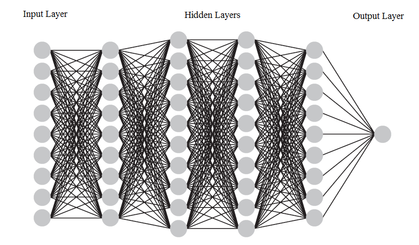
In this work, we use deep forward neural networks to learn the predictors $\pmb{V}$. The artificial neural network was originally developed to emulate the learning ability of the biological neuron system. One can trace the initial concept of artificial neural networks back to the 1940s (see McCulloch and Pitts 1943). To date, the neural network has become a powerful machine learning tool and has been successfully employed in a wide range of applications. The basic mathematical model of the feedforward neural network consists of a series of layers—the input, hidden, and output layers. A deep feedforward neural network can be constructed by adding more hidden layers between the input layer and the output layer. The number of hidden layers is referred to as the depth of the deep neural network. Figure 1 shows a graphical representation of a deep feedforward neural network with nine input variables and four hidden layers. The feedforward neural network along with other types of deep neural networks are collectively known as deep learning methods. Notwithstanding that each individual neuron has little learning capability, when functioning cohesively together, deep neural networks have shown tremendous learning ability and computational power to predict complex nonlinear relationships. For that reason, deep feedforward neural networks serve as a powerful technique for approximating regression functions with multiple regressors. We refer the reader to Schmidhuber (2015) and Goodfellow, Bengio, and Courville (2016) for a comprehensive discussion of deep learning methods.

Figure 1.Graphical illustration of a deep forward neural network.

When a deep feedforward neural network is used to form the predictors in a GLM, the vector of predictors $\pmb{V}$ in (7) takes the form

$$\begin{aligned} \pmb{V} = h_L(\pmb{W}_L, h_{L-1}(\pmb{W}_{L-1},\cdots,h_1(\pmb{W}_{1},\pmb{X}))), \end{aligned}\tag{8}$$

where $\{\pmb{W}_l: l=1,\ldots,L\}$ is a set of weight matrices. Expression (8) is evaluated recursively from the first layer to the last hidden layer in a neural network. Consider a feedforward neural network with $L$ hidden layers; then model (8) amounts to the recursive relation

$$\begin{aligned} \left\{ \begin{array}{l} \pmb{V}_0 = \pmb{X} \\ \pmb{V}_l = h_l(\pmb{W}_l, \pmb{V}_{l-1}), ~~l=1,\ldots,L \\ \pmb{V} = \pmb{V}_L, \\ \end{array} \right. \end{aligned}$$

where $\pmb{V}_l$ is the output from the $l$th hidden layer and forms the inputs for the $(l+1)$th hidden layer. The function $h_l(\pmb{W}_l, \pmb{V}_{l-1})$ is assumed to be of the form $h_l(\pmb{W}_l\pmb{V}_{l-1})$, where $h_l$ is known as the activation function. The activation function is a scalar function and applies to a vector component-wisely. Matrix $\pmb{W}_l$ connects layer $l-1$ to layer $l$, and takes form

$$\begin{aligned} \pmb{W}_l = \left( \begin{array}{ccc} w_{l,11} & \cdots & w_{l,1k_{l-1}} \\ \vdots & \ddots & \vdots \\ w_{l,k_{l}1} & \cdots & w_{l,k_lk_{l-1}} \\ \end{array} \right), \end{aligned}\tag{9}$$

where $k_l$, for $l\in \{1,\ldots,L\}$, denotes the number of neurons in the $l$th hidden layer with $k_0=p$. It is critical to note that the $k$th column of $\pmb{W}_l$ quantifies the effects of the $k$th neuron in the $(l-1)$th layer, and the $k$th row of $\pmb{W}_l$ corresponds to the weights that the $k$th neuron in the $l$th layer receives from all the neurons in the previous layer.

Relations (7) and (8) together form the deep GLM that allows us to efficiently capture the important nonlinear effects of the original raw covariates $\pmb{X}$ on the conditional mean of response $Z$. To be more explicit on model parameters, we rewrite (7) as

$$\begin{aligned} g(\mu) = \eta(\pmb{X},\pmb{w},\pmb{\beta}) = \pmb{V}'\pmb{\beta}. \end{aligned}\tag{10}$$

Here $\pmb{V}=(V_1,\ldots,V_J)'$ with $V_j=\varphi_j(\pmb{X},\pmb{\omega})$ for $j=1,\ldots,J$, where $\pmb{\omega}=(\pmb{W}_1,\ldots,\pmb{W}_L)$ are the weights up to the last hidden layer and $J=k_L$ is the number of neurons in the last hidden layer. The linear coefficients $\pmb{\beta}$ are the weights in the network that connect $\pmb{V}$ to the output layer, and the link function $g$ can be seen as the associated activation function. The network structure (10) can be modified to provide a more interpretable structure in the network. For instance, one could partition the covariates as $\pmb{X}=(\pmb{X}^{(1)},\pmb{X}^{(2)})$ with the expectation that their effects on $g(\mu)$ are linear and nonlinear, respectively. Then we would specify

$$\begin{aligned} g(\mu) = \pmb{X}^{(1)}\pmb{\beta}^{(1)} + \eta(\pmb{X}^{(2)},\pmb{w},\pmb{\beta}^{(2)}), \end{aligned}\tag{11}$$

where coefficients $\pmb{\beta}^{(1)}$ capture the linear effects of $\pmb{X}^{(1)}$, and coefficients $\pmb{\beta}^{(2)}$ capture the nonlinear effects of $\pmb{X}^{(2)}$.

In the frequency-severity model, we specify two deep GLMs, one for claim frequency, $f_N(n|\pmb{X})$, and the other for the conditional average claim severity, $f_{\bar{Y}|N}(\bar{y}|n,\pmb{X})$. In the frequency model, the original raw covariates $\pmb{X}$ are used as input variables in the deep neural network. In contrast, the augmented covariates $\tilde{\pmb{X}}=(N,\pmb{X})$ are used as input variables for the network in the average severity model. One interesting application of model 11) in the severity model is to consider the partition $\pmb{X}^{(1)}=N$ and $\pmb{X}^{(2)}=\pmb{X}$, which allows us to examine whether the effect of claim frequency on average claim severity is linear.

In the dependent frequency-severity model, we approximate the systematic components for $N$ and $\bar{Y}$ using deep neural networks. The proposed deep two-part model nests the linear model considered by Garrido, Genest, and Schulz (2016) as a special case. Specifically, those authors assumed that the systematic components for both $N$ and $\bar{Y}$ are linear combinations of covariates such that

$$\begin{aligned} &\eta_N(\pmb{X},\pmb{\beta}_N)=\pmb{X}'\pmb{\beta}_N \\ &\eta_{\bar{Y}}(N,\pmb{X},\pmb{\beta}_{\bar{Y}}) = \pmb{X}'\pmb{\beta}_Y + \rho N. \end{aligned}$$

In this case, we have $\pmb{\beta}_{\bar{Y}}=(\pmb{\beta}_Y,\rho)$ with parameter $\rho$ quantifying the impact of claim frequency on average claim severity. The model is formulated in such a manner that $\mu_{\bar{Y}|N}=\mu_Y$ when $\rho=0$. The linear model can be obtained through a neural network without hidden layers—thus it can be viewed as a degenerated case of the deep learning method.

3. Introducing sparsity for the deep two-part model

Suppose the insurance claims data are available for $m$ different classes of policyholders. Assume that policyholder $i\in\{1,\ldots,m\}$ has $N_i$ claims during the observation period. The individual claim amount for the $j$th claim, for $j=1,\ldots,N_i$, is denoted by $Y_{ij}$, and the average claim severity is $\bar{Y}_i=\sum_{j=1}^{N_i}Y_{ij}/N_i$ for $N_i>0$. Further, let $\pmb{X}_i=(X_{i1},\ldots,X_{ip})'$ be the vector of exogenous rating variables for class $i$. We assume that $N_i$ is Poisson with mean $\lambda_i$, and $Y_i$ is gamma with mean $\mu_i$ and variance $\phi\mu_i^2$. Both $N_i$ and $\bar{Y}_i$ are specified by the proposed deep GLM in Section 2 with a log link function as follows:

$$\begin{aligned} \mu_{N_i} &= \lambda_i = \exp(\eta_N(\pmb{X}_i,\pmb{w}_N,\pmb{\beta}_N))\\ \phi_{N_i} &= 1\\ \mu_{\bar{Y}_i|N_i} &= \left\{ \begin{array}{ll} \exp(\rho N_i+ \log(\mu_{Y_i})) & {\rm Linear~ effect~ of~ } N_i \\ \exp(\eta_{\bar{Y}}(\tilde{\pmb{X}}_i,\pmb{w}_{\bar{Y}},\pmb{\beta}_{\bar{Y}})) & {\rm Nonlinear~ effect~ of~ } N_i \\ \end{array} \right.\\ \phi_{\bar{Y}_i|N_i} &= \phi/N_i. \end{aligned}$$

In the above, $\mu_{Y_i}=\exp(\eta_{Y}(\pmb{X}_i,\pmb{w}_{Y},\pmb{\beta}_Y)))$ and $\tilde{\pmb{X}}_i=(N_i,\pmb{X}_i)$. The systematic components $\eta_{N}(\cdot)$ and $\eta_{Y}(\cdot)$ or $\eta_{\bar{Y}}(\cdot)$ are specified using the deep neural network model (10). When claim frequency has no effect on average claim severity, we have $\mu_{\bar{Y}_i|N_i}=\mu_{Y_i}$. This relation is reflected by $\rho=0$ in the linear effect model and is implicit in the nonlinear effect model.

In the following, we introduce a regularization method for variable selection in neural networks. We discuss variable selection for numeric and categorical rating variables separately. In the interest of frequency-severity dependence, the method could also allow us to test the nonlinear effect of claim frequency on average claim severity.

3.1. Variable selection in neural networks

Variable selection is often of primary interest in statistical inference but has not received much attention in the deep learning literature. In the context of the deep two-part model, we use the term variable selection to refer to the selection of original raw covariates $\{X_j: j=1,\ldots,p\}$ instead of predictors $\{\varphi_j(\pmb{X}): j=1,\ldots,m\}$ to be included in the model. To develop intuition, we first assume that all raw covariates are continuous, and then extend the idea to the case of categorical covariates.

In a deep neural network, the effect of a covariate $X_j$ on the response is modeled using complex nonlinear transformations through hidden layers. The lack of effect of $X_j$ on the response suggests that the input variable carries no information to any neuron in the first hidden layer of the neural network. In the deep two-part model, we would expect the weights associated with $X_j$ in the first hidden layer to all be equal to zero. Because of this observation, we propose using a group lasso penalty in the loss function of the deep neural network to achieve variable selection.

Let $\pmb{\theta}$ denote the model parameters, i.e., $\pmb{\theta}=(\pmb{\omega}_N,\pmb{\beta}_N,\pmb{\omega}_{\bar{Y}},\pmb{\beta}_{\bar{Y}},\phi)$. Given data $\{(n_i,\bar{y}_i,\pmb{x}_i): i=1,\ldots,m\}$, the log-likelihood function can be written as follows:

$$\small{\begin{aligned} l(\pmb{\theta}) &= \sum_{i=1}^{m} \log(f_{N,\bar{Y}}(n_i,\bar{y}_i|\pmb{x}_i)) \nonumber\\ &=\sum_{i=1}^{m} \log(f_N(n_i|\pmb{x}_i)) + \sum_{i=1}^{m} \log(f_{\bar{Y}|N}(\bar{y}_i|n_i,\pmb{x}_i)) \nonumber\\ &\propto \sum_{i=1}^{m} \left\{n_i\log(\mu_{N_i})- \mu_{N_i}\right\} \nonumber\\ &~~~~+ \frac{1}{\phi}\sum_{i=1}^m n_i\left\{\log\left(\frac{\bar{y}_i}{\mu_{\bar{Y}_i|N_i}}\right)-\frac{\bar{y}_i}{\mu_{\bar{Y}_i|N_i}}\right\} \nonumber\\ &~~~~+\sum_{i=1}^{m}\left\{\frac{n_i}{\phi}\log\left(\frac{n_i}{\phi}\right) - \log\Gamma\left(\frac{n_i}{\phi}\right)\right\}. \end{aligned}\tag{12}}$$

The loss function of the deep two-part model is defined as the sum of the negative log-likelihood function of the data and the group lasso penalty. Let $\pmb{W}_f$ and $\pmb{W}_s$ be the weight matrices connecting the input layer and the first hidden layer in the deep GLMs for claim frequency and average claim severity, respectively. Both matrices take the form of (9). Denote $\pmb{w}_{f,X_j}$ and $\pmb{w}_{s,X_j}$ as the weights associated with covariate $X_j$ for $j\in\{1,\ldots,p\}$. We note that $\pmb{w}_{f,X_j}$ and $\pmb{w}_{s,X_j}$ are the $j$th column of $\pmb{W}_f$ and $\pmb{W}_s$, respectively. The loss function can be expressed as

$$\begin{aligned} L(\pmb{\theta}) &= -l(\pmb{\theta}) + \lambda_f \sum_{j=1}^{p}||\pmb{w}_{f,X_j}||_2 \\ &\quad + \lambda_s \sum_{j=1}^{p}||\pmb{w}_{s,X_j}||_2, \end{aligned}\tag{13}$$

where $\lambda_f$ and $\lambda_s$ are the tuning parameters in the claim frequency and the average claim severity models, respectively, and $||\pmb{w}_{f,X_j}||_2$ and $||\pmb{w}_{s,X_j}||_2$ are the Euclidean norms of the vectors $\pmb{w}_{f,X_j}$ and $\pmb{w}_{s,X_j}$, respectively.

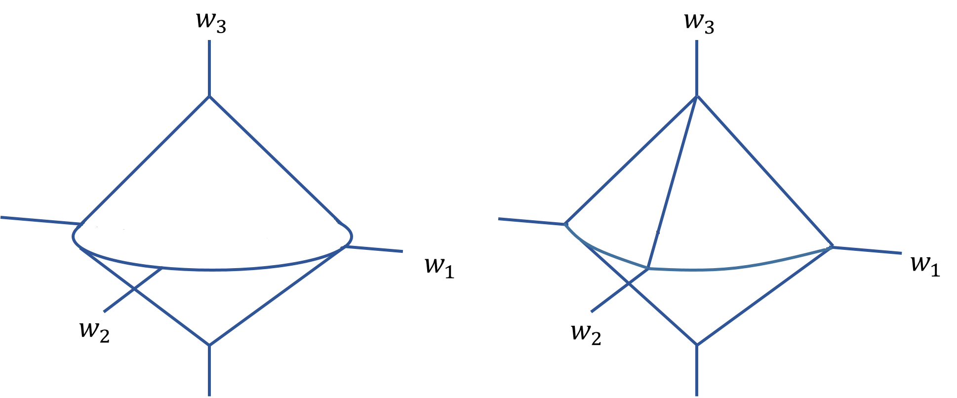
To provide some intuition, we consider a parameter vector $\pmb{w}=(w_1,w_2,w_3)'$ with two groups $\{w_1,w_2\}$ and $\{w_3\}$. We exhibit the unit constraint region $\sqrt{w_1^2+w_2^2}+|w_3|\le 1$ in the left panel of Figure 2. The plot suggests that the Euclidean norm will introduce sparsity at the group level. In loss function (13), the Euclidean norm ensures that either the entire vector (either $\pmb{w}_{f,X_j}$ or $\pmb{w}_{s,X_j}$ depending on the value of $\lambda_f$ or $\lambda_s$, respectively) will be zero or all its elements will be nonzero. In addition, when there is only one neuron in the first hidden layer (i.e., $k_1=1$) in the neural network for claim frequency or average claim severity, the shrinkage reduces to the ordinary lasso, i.e., $||\pmb{w}_{f,X_j}||_2 = |\pmb{w}_{f,X_j}|$ or $||\pmb{w}_{s,X_j}||_2=|\pmb{w}_{s,X_j}|$. As a result, the group lasso allows us to perform variable selection in that all weights for a covariate will be shrunk to zero if the covariate does not have enough predictive power to warrant its inclusion in the neural network.

Figure 2.Constraint regions for the group LASSO (left panel) and the sparse group LASSO (right panel). The two groups in parameters are $\left\{w_1, w_2\right\}$ and $\left\{w_3\right\}$.

The parameters in a deep neural network are found to minimize the loss function, which measures the discrepancy between observed values and predicted values of the outcome. The training process of deep neural networks can be challenging because the loss function is nonconvex, contains local minima and flat spots, and is highly multidimensional due to the large number of parameters. Gradient descent is the general algorithm used to solve the optimization where the gradient is computed via backpropagation (Rumelhart, Hinton, and Williams 1986). We employ the mini-batch gradient descent algorithm with the learning rate for each parameter computed using adaptive moment estimation (see Kingma and Ba 2014). The process is iterative, and in each iteration parameters are updated using only a random subset, or mini-batch, of the training data. Fitting a neural network may require many complete passes through the entire training data. In the two-part model, we can partition the parameters into three components such that $\pmb{\theta}=(\pmb{\theta}_f,\pmb{\theta}_s,\phi)$, where $\pmb{\theta}_f=(\pmb{w}_N,\pmb{\beta}_N)$ summarizes the parameters in the mean of claim frequency, and $\pmb{\theta}_s=(\rho,\pmb{w}_{Y},\pmb{\beta}_Y)$ or $\pmb{\theta}_{\bar{Y}}=(\pmb{w}_{\bar{Y}},\pmb{\beta}_{\bar{Y}})$ summarizes the parameters in the mean of average claim severity. It is important to note that the estimations of $\pmb{\theta}_f$ and $\pmb{\theta}_s$ are separable and both are independent of $\phi$. Specifically, the system of scores or gradients for $\pmb{\theta}_f$ and $\pmb{\theta}_s$ are shown as

$$\begin{aligned} \Delta_f &= \sum_{i=1}^{m}\frac{\partial \mu_{N_i}}{\partial \theta_{f,k}} (n_i-\mu_{N_i}) \\ &\quad + \lambda_f \sum_{j=1}^p \frac{\theta_{f,k} 1\{\theta_{f,k}\in \pmb{w}_{f,X_j}\}}{||\pmb{w}_{f,X_j}||_2},~~k=1,\ldots,|\pmb{\theta}_f|\\ \Delta_s &= \sum_{i=1}^{m} \frac{\partial \mu_{\bar{Y}_i|N_i}}{\partial \theta_{s,k}} n_i(\bar{y}_i-\mu_{\bar{Y}_i|N_i}) \\ &\quad + \lambda_s\phi \frac{\theta_{s,k} 1\{\theta_{s,k}\in \pmb{w}_{s,X_j}\}}{||\pmb{w}_{s,X_j}||_2},~~k=1,\ldots,|\pmb{\theta}_s| , \end{aligned}$$

where $|A|$ denotes the cardinality of set $A$. The score equations also suggest that variable selection can be done independent of the dispersion parameter. The tuning parameters are determined using cross-validation with the rule of thumb being the one-standard-error rule. We refit the deep two-part model once the important variables are selected. We can estimate the dispersion parameter in different ways. We estimate the dispersion as part of the training process in the neural network by minimizing the loss function. As an alternative, the dispersion parameter $\phi$ can be estimated from the Pearson residuals as in conventional GLMs:

$$\begin{aligned} \hat{\phi} = \frac{1}{m-|\pmb{\theta}_s|} \sum_{i=1}^m n_i \left(\frac{\bar{y}_i-\hat{\mu}_{\bar{Y}_i|N_i}}{\hat{\mu}_{\bar{Y}_i|N_i}}\right)^2, \end{aligned}\tag{14}$$

where $\hat{\mu}_{\bar{Y}_i|N_i}$ is the fitted value of $\mu_{\bar{Y}_i|N_i}$.

The proposed deep two-part model has a couple of unique features that differ from the traditional frequency-severity models. First, one must specify an activation function for each hidden layer in the deep neural network. One often selects nonlinear activations because the nonlinearity can accommodate complex relations between inputs and output. Second, training a neural network involves decisions about the hyperparameters, such as the number of hidden layers, the number of neurons within a hidden layer, and the learning rate. These hyperparameters control the bias–variance trade-off in that whereas a neural network with more neurons and more layers provides a better approximation of the unknown function, it is prone to overfit the unique characteristics of the training data and the predictive performance cannot be generalized to the independent test data. The rule of thumb for tuning the hyperparameters is to use cross-validation techniques to evaluate the predictive performance of the neural network for a grid of values from the hyperparameters.

3.2. Selecting categorical covariates

In the previous section, we assumed that all covariates are continuous variables. In actuarial and insurance applications, many rating variables are naturally categorical. For instance, one can think of roof type in homeowner insurance, occupational class in worker’s compensation, and vehicle make in automobile insurance, among others. In this section, we propose two strategies to perform variable selection for categorical input variables in the deep two-part model, depending on how a categorical input is incorporated in the neural network.

There are two strategies for incorporating categorical inputs in a neural network: one-hot encoding and categorical embedding. One-hot encoding is the most common approach in the statistical learning method, where one expands a categorical variable into a series of dummy variables. Consider a categorical input variable $X$ that has $T$ levels with values $\{c_t: t=1,\ldots,T\}$. One-hot encoding can be formulated as a function $h$ that maps the categorical variable into a vector of binary variables:

$$\begin{aligned} h: X \mapsto \pmb{\delta} = (\delta_{X,c_1},\ldots,\delta_{X,c_T})', \end{aligned}\tag{15}$$

where $\delta_{X,c_t}$, for $t=1,\ldots,T$, is the Kronecker delta, which equals 1 if $X=c_t$ and 0 otherwise. One-hot-encoded categorical input variables are ready to use in deep neural networks. The method is appropriate when the categorical variable has a relatively small number of levels, such as gender and marital status in our application.

Categorical embedding is an alternative method to incorporate categorical input variables in a neural network (see Shi and Shi 2023). The method can be formulated as a function $e$ that maps the categorical variable into a real-valued vector. For the categorical variable $X$ with $T$ levels, the embedding function of a $d$-dimensional embedding space is given by

$$\begin{aligned} e: X \mapsto \pmb{\Omega} \times \pmb{\delta}, \end{aligned}\tag{16}$$

where $\pmb{\delta}$ is the one-hot-encoded vector and $\pmb{\Omega} \in \mathbb{R}^{d\times T}$ is known as the embedding matrix. The matrix $\pmb{\Omega}$ can be viewed as a $d$-dimensional numerical representation of the categorical variable, and the $t$th column of $\pmb{\Omega}$ represents the $t$th category of $X$ for $t=1,\ldots,T$. To show this for the $i$th data point with $X_i=c_t$, we note

$$\begin{aligned} e(c_t) &= \pmb{\Omega} \times \pmb{\delta}_i\\ &= \left( \begin{array}{ccc} \omega_{11} & \cdots & \omega_{1T} \\ \vdots & \ddots & \vdots \\ \omega_{d1} & \cdots & \omega_{dT} \\ \end{array} \right) \times \left( \begin{array}{c} \delta_{X_i,c_1} \\ \vdots \\ \delta_{X_i,c_T} \\ \end{array} \right) \\&= \left( \begin{array}{c} \omega_{1t} \\ \vdots \\ \omega_{dt} \\ \end{array} \right), \end{aligned}\tag{17}$$

for $t\in\{1,\ldots,T\}$. The dimension of embedding space is bounded between 1 and $T-1$, i.e., $1\le d\le T-1$.

The categorical embedding method is recommended when the categorical variable has a large number of levels. Some examples are vehicle model and make, postal code, and occupational class. The method maps each categorical variable into a real-valued representation in the Euclidean space. For categorical variables with a large number of levels, the dimension of the embedding space is typically much smaller than the number of categories. Compared with one-hot encoding, categorical embedding leads to a dimension reduction and thus mitigates overfitting. More important, the one-hot-encoded binary vectors for different levels of a categorical variable are orthogonal and hence cannot reflect the similarities among them. In contrast, the categories with similar effects are close to each other in the embedding space and thus the intrinsic continuity of the categorical variable is naturally revealed.

When categorical embedding is used for categorical input $X$, the $d\times T$ parameters in the embedding matrix $\pmb{\Omega}$ can be learned along with the weight parameters in a deep learning model. In implementation, one adds an embedding layer for a given categorical input between the input layer and the hidden layer in the neural network architecture. The embedding layer consists of $d$ neurons so as to map the categorical input with $T$ levels into a $d$-dimensional embedding space. Specifically, the embedding layer uses the one-hot-encoded categorical variable as inputs and then applies an identity activation function to compute the outputs. When there is more than one categorical input variable, each categorical input is mapped into its own embedding space and the dimension of embedding space can be different across the multiple categorical inputs. Each categorical variable generates an embedding layer in the neural network, and the embedding layers are independent of each other. The outputs from the embedding layer and the continuous input variables are then concatenated. The resulting merged layer is treated as a normal input layer in the neural network, and hidden and output layers can be further built on top of it.

To perform variable selection for categorical inputs in the deep two-part model, we consider two scenarios regarding whether or not categorical embedding is implemented for categorical inputs. When the number of levels of the categorical input is small, we recommend applying the group lasso penalty directly to the one-hot-encoded binary variables without using the embedding layer in the network. For a single categorical input $X$ with $T$ levels, one-hot encoding amounts to $T$ binary input variables in (15). Let $\pmb{w}_{\delta_t}=(w_{\delta_t,1},\ldots,w_{\delta_t,k_1})'$ be the vector of weights in the first hidden layer in the deep architecture of the neural network that is associated with binary inputs $\delta_{X,c_t}$ for $t\in\{1,\ldots,T\}$. Further define as

$$\begin{aligned} \pmb{W}_{\pmb{\delta}} = \left( \begin{array}{c} \pmb{w}'_{\delta_1} \\ \vdots \\ \pmb{w}'_{\delta_S} \\ \end{array} \right) = \left( \begin{array}{ccc} w_{\delta_t,1} & \cdots & w_{\delta_t,k_1} \\ \vdots & \ddots & \vdots \\ w_{\delta_T,1} & \cdots & w_{\delta_T,k_1} \\ \end{array} \right). \end{aligned}\tag{18}$$

If the categorical variable $X$ is not predictive and is not included in the model, all elements in the weight matrix $\pmb{W}_{\pmb{\delta}}$ should be zero. Thus, for variable selection purposes, one employs the Frobenius norm of $\pmb{W}_{\pmb{\delta}}$, denoted by $||\pmb{W}_{\pmb{\delta}}||_F$, in the loss function of the deep neural network. When the number of levels of the categorical input is large, we recommend using categorical embedding and executing variable selection in the embedding space. In a similar manner, we define the weight matrix from the embedding layer to the first hidden layer as

$$\begin{aligned} \pmb{W}_{\pmb{e}} = \left( \begin{array}{ccc} w_{e_1,1} & \cdots & w_{e_1,k_1} \\ \vdots & \ddots & \vdots \\ w_{e_d,1} & \cdots & w_{e_d,k_1} \\ \end{array} \right), \end{aligned}\tag{19}$$

where each row corresponds to a neuron in the embedding space. We impose a regularization of the norm $||\pmb{W}_{\pmb{e}}||_F$ in the loss function. The weight matrix will be shrunk to zero if the categorical variable $X$ is not predictive for the outcome. The above ideas simply generalize to the case of multiple categorical input variables such that a group lasso penalty is employed for each categorical input. In the two-part model, separate penalties are employed for the claim frequency and the average claim frequency.

Figure 3 shows a conceptual illustration of the deep learning network with group lasso regularization for variable selection. We summarize three scenarios in the figure: regularization for a continuous input, a one-hot-encoded categorical input, and a categorical input with embedding. One can think of all layers prior to the variable selection layer as input preprocessing. All preprocessed inputs, both continuous and categorical, are concatenated as inputs for the variable selection. We emphasize that regularization could be applied to any hidden layer to introduce sparsity. In contrast, our focus is to employ group lasso regularization to achieve variable selection for the raw covariates instead of learned features in the deep learning method.

Figure 3.Conceptual exhibition of the sparse deep two-part model.

The application of group lasso in neural networks for variable selection is different from the typical context where the group lasso is employed for a group of variables. In the case of several groups of variables, the number of variables in a group usually varies by group. In contrast, the number of weight parameters is the same for all covariates and is equal to the number of neurons in the first hidden layer. This constraint could be relaxed in an extension of the proposed sparse deep two-part model. Recall that group lasso regularization implies that for a given covariate, if one of the weight parameters is not zero, then all of the weights will be nonzero. This property might not be ideal when the effect of a covariate could be sufficiently represented using a subset of neurons in the first hidden layer. To provide extra flexibility, we could augment the basic group lasso with an additional ordinary lasso penalty, leading to the sparse group lasso regularization as below:

$$\small{\begin{aligned} PL(\pmb{\theta}) &= -l(\pmb{\theta}) \\ &\quad + \lambda_f \sum_{j=1}^{p}\left\{(1-\gamma_f)||\pmb{w}_{f,X_j}||_2+\gamma_f ||\pmb{w}_{f,X_j}||_1\right\} \nonumber\\ \\ &\quad + \lambda_s \sum_{j=1}^{p}\left\{(1-\gamma_s)||\pmb{w}_{s,X_j}||_2+\gamma_s||\pmb{w}_{s,X_j}||_1\right\}, \end{aligned}\tag{20}}$$

with $\gamma_s,\gamma_f \in[0,1]$. The parameters $\gamma_s$ and $\gamma_f$ create a bridge between the group lasso ($\gamma_f=0$ and/or $\gamma_s=0$) and the regular lasso ($\gamma_f=1$ and/or $\gamma_s=1$). The sparse group lasso is designed to achieve sparsity within a group. In the deep two-part model, it allows us to select an important covariate $X_j$ while setting a subset of the weight parameters ($\pmb{w}_{f,X_j}$ for claim frequency and $\pmb{w}_{s,X_j}$ for average claim severity) to be zeros. This intuition is illustrated using the constraint region in the right panel of Figure 2. As the plot suggests, the two parameters in the group $\{w_1,w_2\}$ do not need to be nonzero simultaneously when the group is selected.

Model parameters are obtained by minimizing the loss function. It is important to note that the optimization can be challenging because the error surface is nonconvex, contains local minima and flat spots, and is highly multidimensional due to the large number of parameters. Stochastic gradient descent is the general algorithm to solve the optimization where the gradient is computed via backpropagation. The process is iterative, and in each iteration parameters are updated using only a random subset, or mini-batch, of the training data. Fitting a neural network may require many complete passes through the entire training data.

4. Numerical experiments

This section uses comprehensive simulation studies to investigate the performance of the deep two-part model and variable selection using group lasso. For briefness, we report the results of three representative numerical experiments. The first two studies mimic the claim frequency model—one examines Poisson models that contain only continuous inputs, and the other focuses on variable selection for categorical input variables. The last study considers a conditional gamma model for average claim severity where we demonstrate simultaneous training of the neural network and estimation of the dispersion parameter.

4.1. Claim frequency: Continuous inputs

In this experiment, we have a set of five covariates available for model development such that $X_j \sim Uniform (0,1)$ for $j\in\{1,\dots,5\}$. We assume a Poisson model with a log link function for claim frequency, and we consider both linear and nonlinear settings as follows:

$$\begin{aligned} &Y_i|\pmb{X}_i \sim Poisson(\eta_i) \\ {\rm Linear ~Model:~}& \log(\eta_i) = -0.5 + 0.5 X_{i1} + 1.5 X_{i2} + 4 X_{i3} \\ {\rm Noninear ~Model:~}& \log(\eta_i) = 4 + 3 X_{i1}^{1/2} - 5X_{i2}^{2/3}. \end{aligned}$$

The first model considers a linear combination of covariates in the regression function and uses only the variables $X_1$, $X_2$, and $X_3$ to generate $Y$. The second model considers nonlinear transformations of raw covariates as basis functions, and only the variables $X_1$ and $X_2$ are used to generate $Y$.

To demonstrate variable selection, we fit a deep Poisson model using the random sample generated from the above linear and nonlinear models separately. In both models, we employ basis functions formed by a deep neural network. The neural network uses all five covariates $\{X_j; j=1,\ldots,5\}$ as input variables, and employs a group lasso regularization on the weights of the raw input variables, treating each input as a group. The reported results are based on random samples of 2,000 observations. We use 70% of data to train the deep neural network and 30% of data for validation. The final networks contain one hidden layer with three and six neurons for the linear and nonlinear models, respectively.

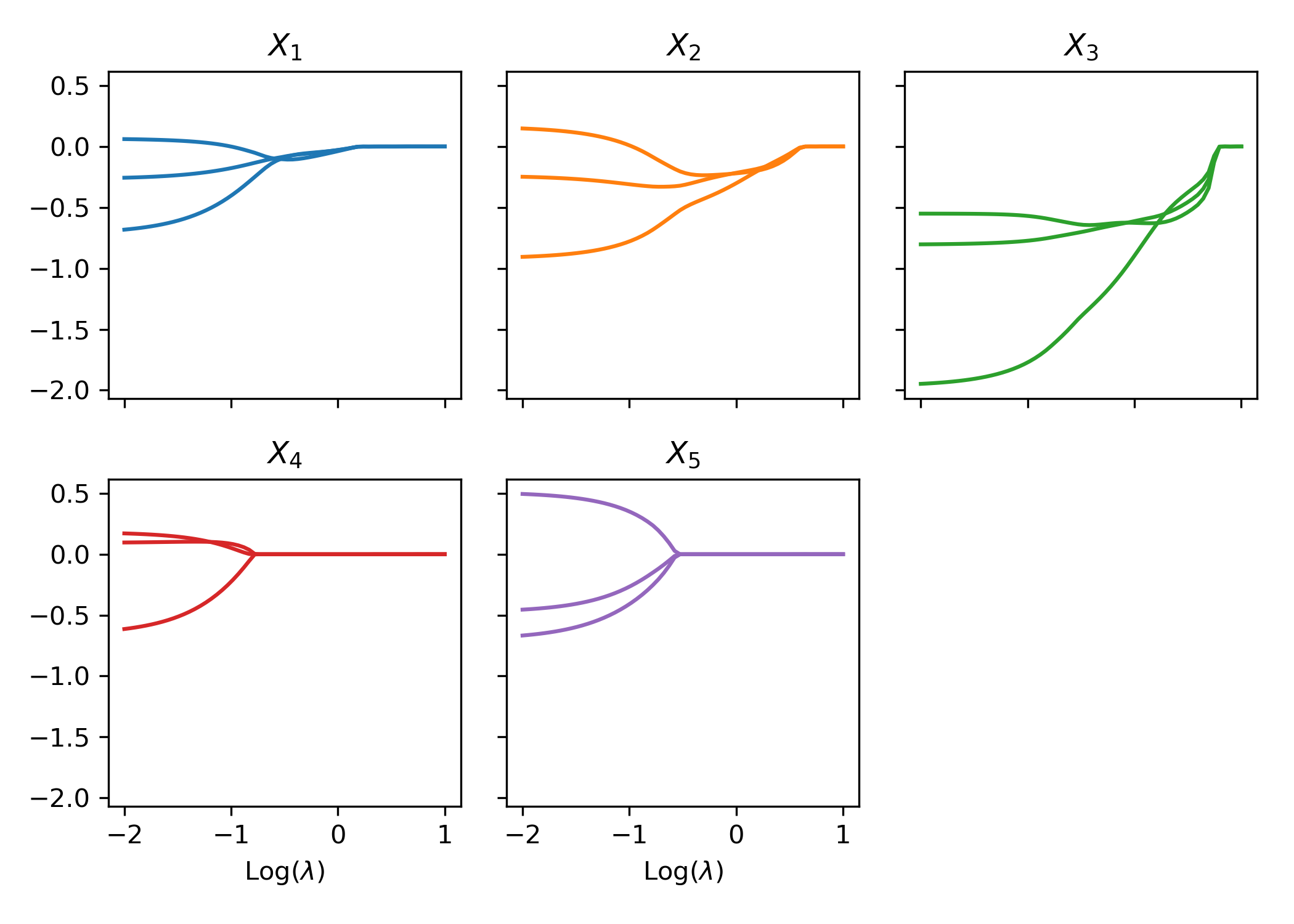
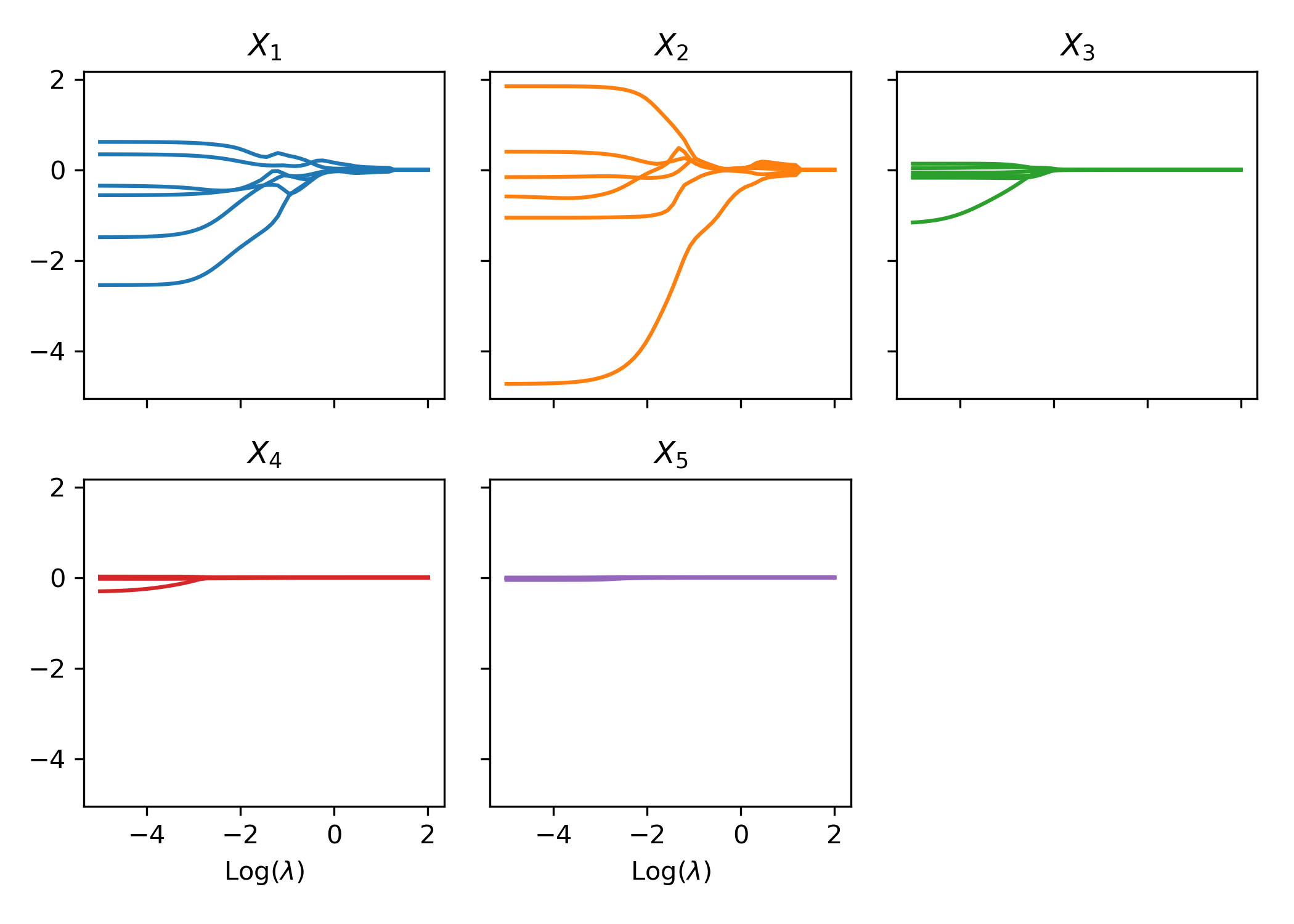
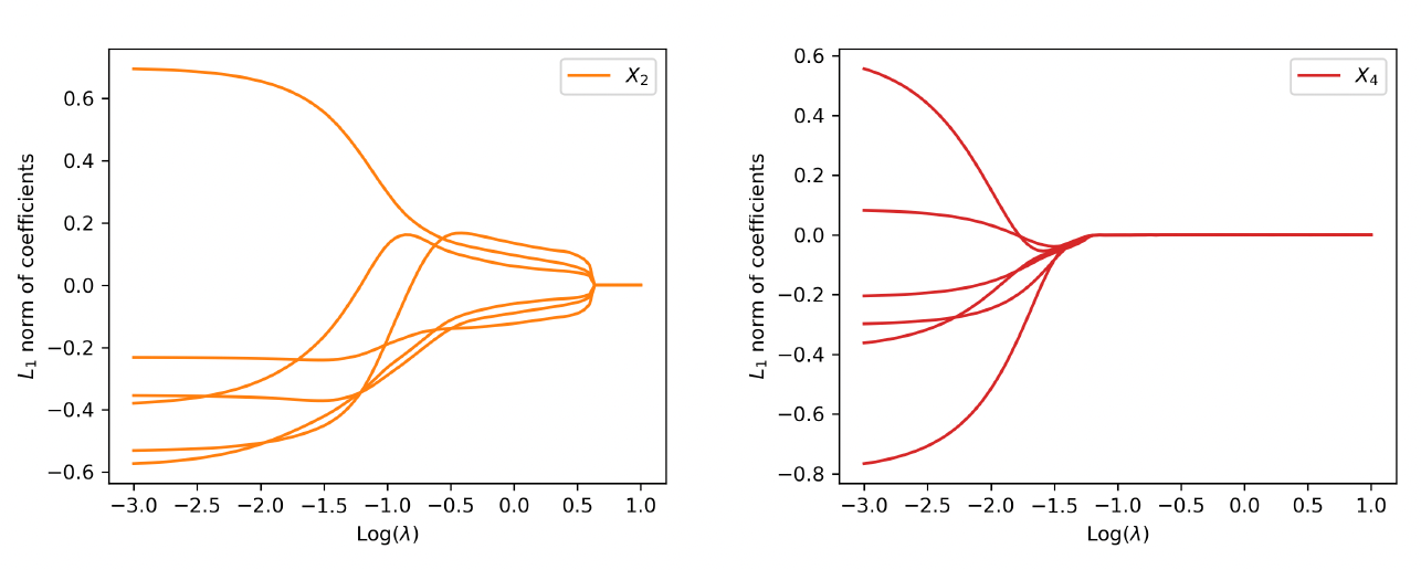
We first examine the performance of the proposed method when data are generated from the linear model. Figure 4 shows the path of the weights for the raw inputs as a function of the tuning parameter in the regularization, where each plot corresponds to the weights for a given covariate. As anticipated, we observe that the regularization introduces sparsity among weights such that all weight parameters are eventually shrunk to zero when the tuning parameter is large enough. More important, the group lasso penalty ensures that the weights associated with the same covariate are either all zero or all nonzero. When the tuning parameter is equal to zero, the weights coincide with the neural network without regularization.

Figure 4.The path of weight parameters for each input variable in the linear Poisson model.

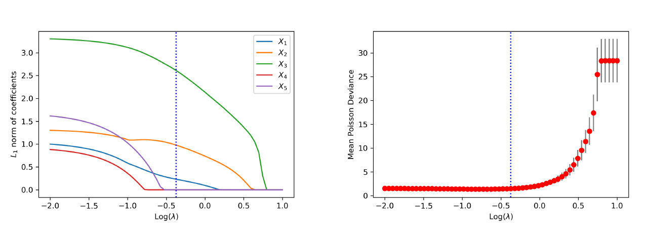
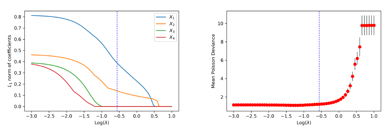
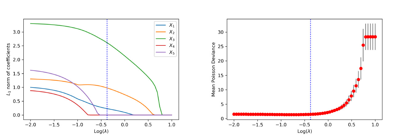
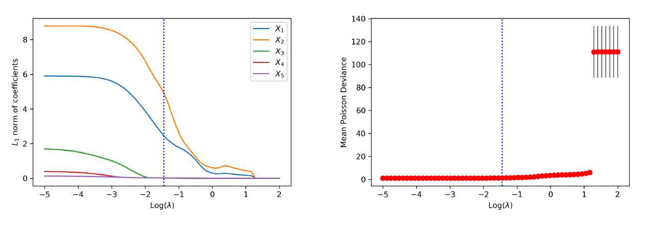
To visualize the shrinkage effects on the raw covariates, we exhibit in the left panel of Figure 5 the path of the $l_1$-norm of the weight vector for each covariate. First, we observe that $X_4$ and $X_5$ are shrunk to zero prior to $X_1$, $X_2$, and $X_3$. The behavior is explained by the fact that $Y$ is generated independent of $X_4$ and $X_5$. Second, the order by which the covariates ($X_1$, $X_2$, and $X_3$) in the true model are shrunk to zero is consistent with the variation of response accounted for by each covariate. For the purpose of variable selection, the optimal tuning parameter is selected using $k$-fold cross-validation. The training data are randomly divided into $k$ groups, or folds. That procedure is repeated for $k$ times, with one of the $k$ folds as the validation set and the remaining $k-1$ folds to train the model each time. For each repetition, the deviance is calculated for a grid of values for the tuning parameter. The right panel of Figure 5 presents the estimated test deviance with error bars by the tuning parameter, where the vertical line corresponds to the model within one standard error of the lowest point on the curve. The same line is exhibited in the left panel, indicating that the one-standard-error rule correctly selects the important covariates.

Figure 5.Variable selection for the linear Poisson model. The left panel shows the $l_1$-norm of weights for individual input variables, and the right panel shows the deviance path using 10 -fold cross-validation.

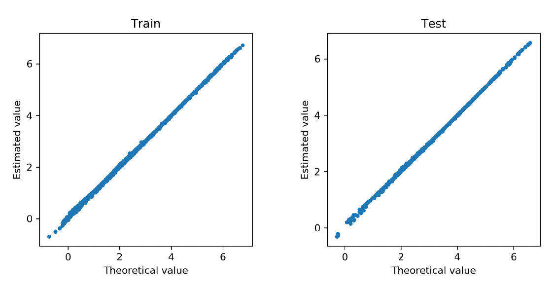
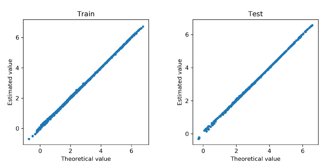
When the data are generated from the nonlinear model, similar conclusions are drawn from the analysis. First, the weights of each covariate are clustered via the group lasso regularization, and the path of shrinkage reflects the relative importance of the covariates. Second, the one-standard-error rule in the cross-validation correctly selects the two covariates in the data generating despite their nonlinear effects. The path of weights for each input and the variable selection performance are reported in Figure 6 and Figure 7, respectively.

Figure 6.The path of weight parameters for each input variable in the nonlinear Poisson model.

Figure 7.Variable selection for the nonlinear Poisson model. The left panel shows the $l_1$-norm of weights for individual input variables, and the right panel shows the deviance path using 10 -fold cross-validation.

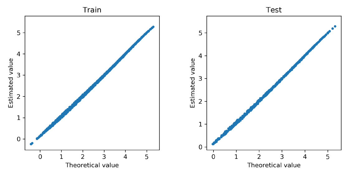
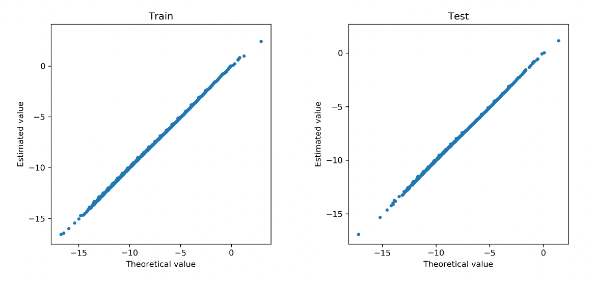
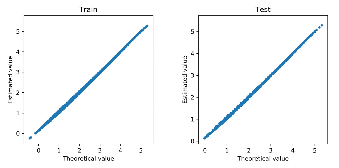
We further examine how accurate the neural network approximates the regression function in Poisson models. To that end, we refit the deep Poisson models using the selected covariates. We obtain the fitted value for each observation in the training data and the predicted value for each observation in the test data. Both fitted and predicted values are compared with the true regression function in the data generating. Figure 8 and Figure 9 show the corresponding scatter plots for the cases of the linear and nonlinear data-generating processes, respectively. In both scenarios, the approximated regression functions from the neural network consistently align with the underlying true regressions. We further report in Table 1 the mean deviance for the training and test data in both linear and nonlinear scenarios. The deviance measures the overall goodness of fit of the model. For comparison, we present the mean deviance for both the Poisson model and the deep Poisson model. In both cases, the mean deviances in the training and test data are in the same order. Consistent with the scatter plots, the mean deviances from the neural networks and the true models are closely aligned with each other. In conclusion, the Poisson model with the basis functions formed by the deep neural networks provides accurate approximation for the true regression function, and the group lasso penalty allows one to select important covariates in the deep learning method.

Figure 8.Comparison of the linear Poisson and deep Poisson models. The left panel compares the fitted value from the training data and the right panel compares the predicted value from the test data.

Figure 9.Comparison of the nonlinear Poisson and deep Poisson models. The left panel compares the fitted value from the training data and the right panel compares the predicted value from the test data.

4.2. Claim frequency: Categorical inputs

This experiment examines the variable selection for categorical inputs in the deep learning method. As discussed in Section 3.2, categorical inputs can be incorporated in a neural network using either one-hot encoding or categorical embedding. The former is more appropriate when the categorical input has a small number of levels, and the latter is preferred when the categorical input has a large number of levels. As a result, variable selection is performed in the input layer or the embedding layer in the neural network. We investigate both cases using numerical experiments. Specifically, we consider the data-generating process

$$\begin{aligned} Y_i|\pmb{X}_i &\sim Poisson(\eta_i) \\ \log(\eta_i)& = 1 + 2 X_{i1}^{1/2} + X_{i2}, \end{aligned}$$

where $X_1\sim Uniform(0,1)$ and $X_2\sim Bernoulli(0.6)$. We use a random sample of 2,000 observations, with 70% of the data as the training set and the remaining 30% as the test set. We fit two deep Poisson models using the training data. The two neural networks use $Y$ as the output variable but use different sets of variables as inputs.

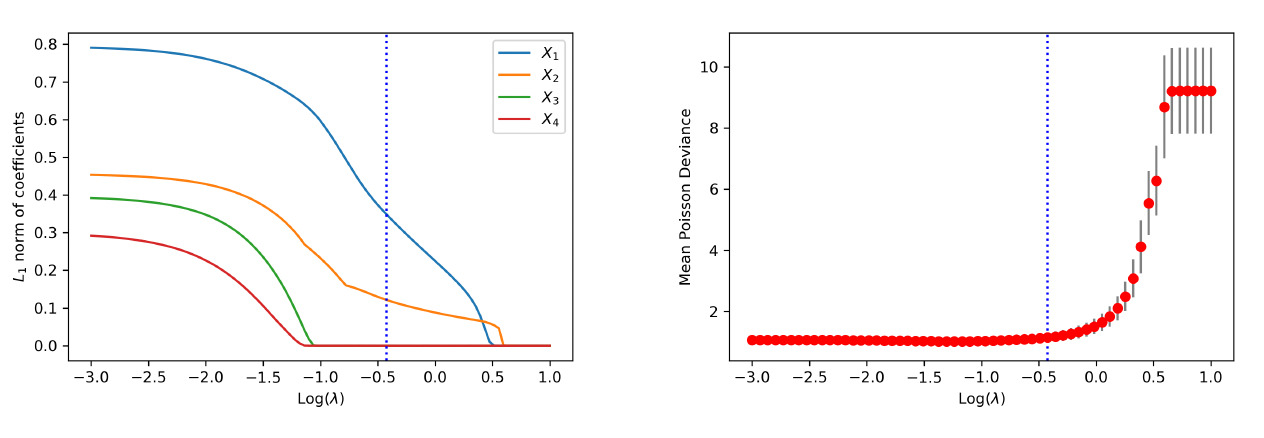
In the first model, two additional covariates, in addition to $X_1$ and $X_2$, are included as inputs for the neural network. One, $X_3\sim Uniform(0,1)$, is a continuous variable, and the other, $X_4$, is a categorical variable with three levels from a multinomial distribution. To incorporate $X_4$ in the neural network, we use one-hot encoding to transform the categorical variable into three binary variables. The final trained network contains one hidden layer with three neurons. The results on variable selection are presented in Figure 10. The left panel shows the $l_1$-norm of weights associated with each covariate in the first hidden layer. It is noted that covariates $X_3$ and $X_4$ are shrunk to zero prior to $X_1$ and $X_2$. The right panel shows the estimated test deviance with error bars using the 10-fold cross-validation by a grid of tuning parameters. The vertical lines in both plots correspond to the tuning parameter based on the one-standard-error rule. The one-standard-error rule accurately selects the covariates used in the data-generating process.

Figure 10.Variable selection for categorical inputs using one-hot encoding. The left panel shows the $l_1$-norm of weights for individual input variables, and the right panel shows the deviance path using 10 -fold cross-validation.

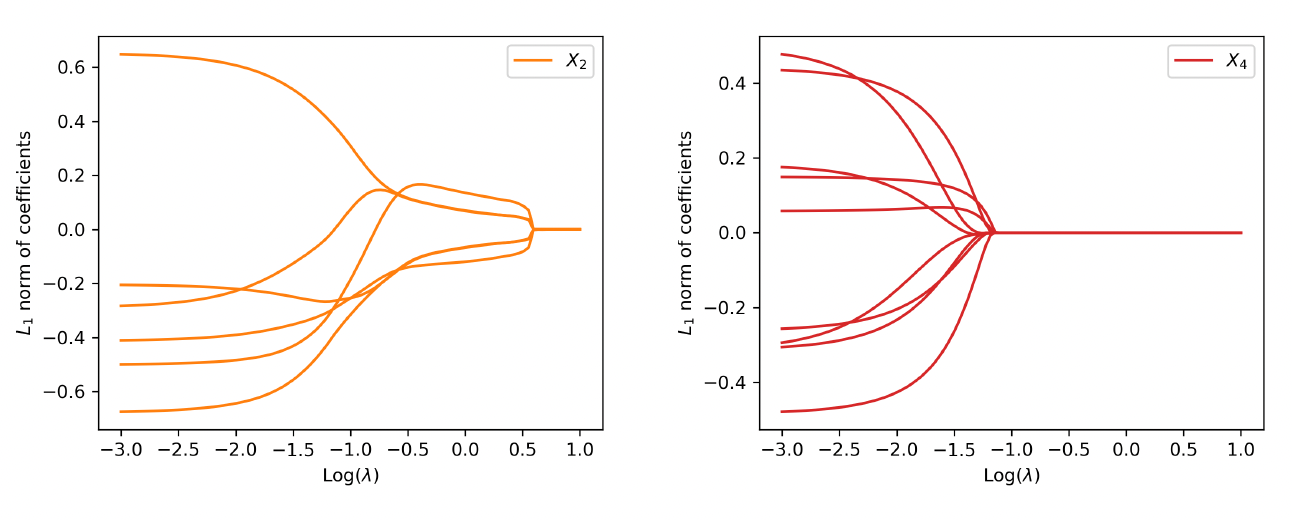
To emphasize the difference from continuous covariates, we present the path of weights associated with the two categorical inputs $X_2$ and $X_4$ in Figure 11. Among them, $X_2$ has two levels and are selected, and $X_4$ has three levels and are not selected. Because of the one-hot encoding, there are six and nine weights associated with $X_2$ and $X_4$, respectively. This differs from a continuous input in the network architecture. For a continuous input, the group lasso applies to a single neuron in the input layer. In contrast, for the one-hot-encoded categorical input, the group lasso applies to multiple neurons in the input layer that correspond to the encoded binary variables.

Figure 11.The path of weight parameters for $X_2$ and $X_4$ in the one-hot encoding model.

In the second model, we also use two additional covariates, $X_3$ and $X_4$, as inputs for the neural network. The continuous covariate $X_3$ remains the same as in the first model. In contrast, the categorical $X_4$ is generated from a multinomial distribution with 50 levels. For the two categorical covariates, we employ one-hot encoding for $X_2$ and categorical embedding for $X_4$. In the neural network, the variable $X_4$ is projected to a two-dimensional Euclidean space and the embeddings are concatenated with other covariates as regular inputs. These inputs are fed into a hidden layer with three neurons. Different from the above experiment, the group lasso applies to the embeddings of $X_4$ and thus variable selection is performed at the embedding layer. Figure 12 reports the results on variable selection. The left panel shows the path of the $l_1$-norm of weights for each covariate, and the right panel shows the choice of the tuning parameter in the regularization based on cross-validation. We note that the categorical variable $X_4$ is identified as nonpredictive when the embeddings are regularized. Figure 13 further shows the detailed path of weights for the two categorical variables. The path for $X_2$ is similar to Figure 11 since one-hot encoding is used for both cases. In contrast, the path for $X_4$ corresponds to the weights in the embedding layer, and thus there are six of them as opposed to $50\times 3=150$ under the one-hot encoding. Overall, we observe that the variable selection for categorical inputs in the neural network can be successfully implemented using both one-hot and categorical embedding methods.

Figure 12.Variable selection for categorical inputs using categorical embedding. The left panel shows the $l_1$-norm of weights for individual input variables, and the right panel shows the deviance path using 10 -fold cross-validation.

Figure 13.The path of weight parameters for $X_2$ and $X_4$ in the categorical embedding model.

4.3. Average claim severity

The third experiment considers a deep gamma model as an example of continuous outcome in the exponential family. To mimic the conditional severity model in Section 2, we consider the following data-generating process:

$$\begin{aligned} N_i|X_i &\sim Poisson(\eta_i)\\ \log(\eta_i)& = 2 + X^{1/2}_{i}\\ \bar{Y}_i|(N_i,X_i) &\sim Gamma (\mu_i,\phi_i) \\ \log(\mu_i)& = 4 + X^{1/2}_{i} -2 N_i^{2/3}\\ \phi_i & = \phi/N_i =4/N_i, \end{aligned}$$

where $X\sim Uniform(0,1)$. The gamma distribution is parameterized using mean $\mu_i$ and dispersion $\phi_i$, both of which are subject specific. The heterogeneity in mean is accounted for by the rating variable $X$ and the claim frequency $N$, and the heterogeneity in dispersion is due to the weight.

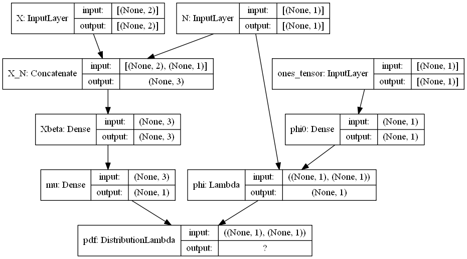
We fit a deep gamma model where the basis function in the regression equation for $\mu_i$ is formed using a deep neural network. In the neural network, variables $X$ and $N$ are used as inputs, and $\bar{Y}$ as the output. The loss function is defined as the negative log-likelihood function. We report results based on a random sample of 4,000 observations, of which 70% are used for training and 30% for testing. We consider two methods for estimating the dispersion parameter $\phi$. First, $\phi$ is estimated in the training process for the neural network. To implement this strategy, we employ the architecture in Figure 14 in the deep learning method. In particular, the claim frequency is, on the one hand, concatenated with covariates to form the inputs fed into the dense layers. On the other hand, the claim frequency is an input in the lambda layer that will serve as a weight in the dispersion. Second, the dispersion parameter is estimated based on $\chi^2$ statistics using (14).

Figure 14.The neural network architect in the deep gamma model.

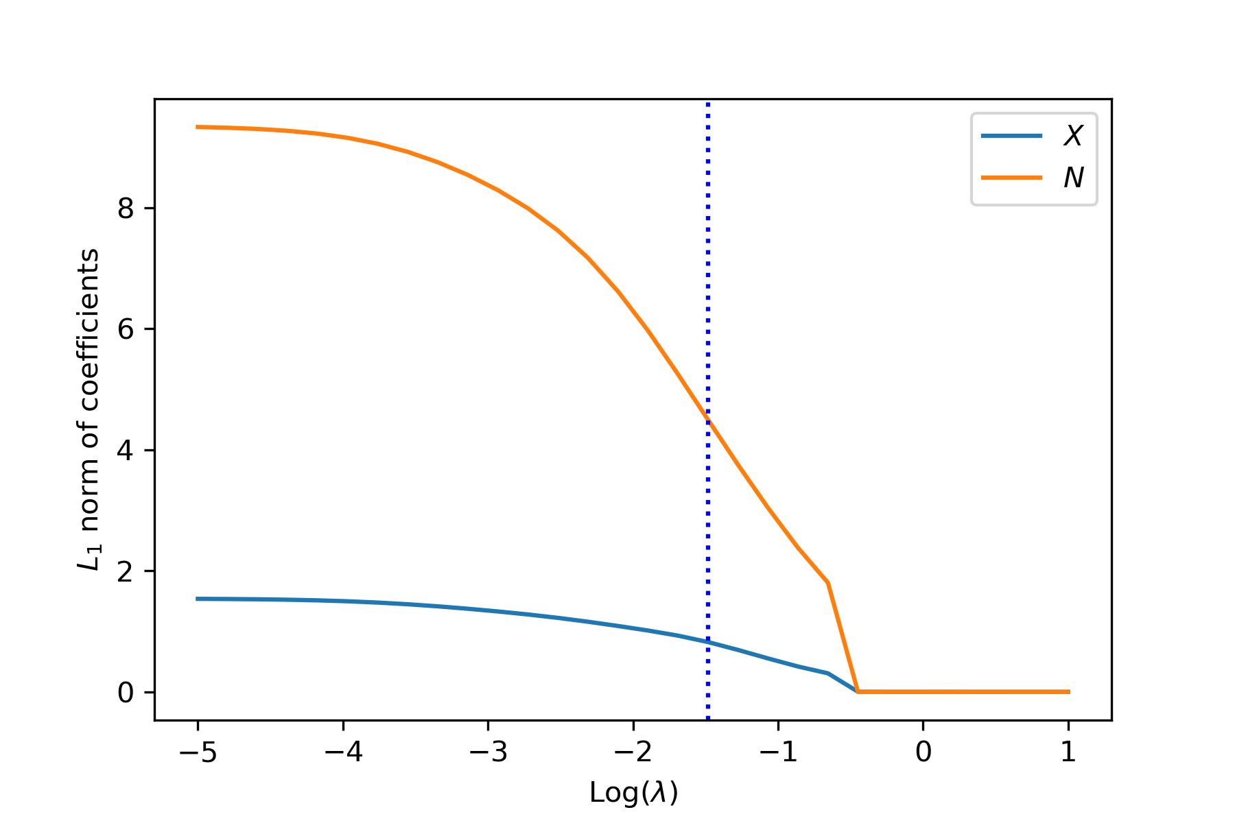
Figure 15 exhibits the path of the $l_1$-norm of weights for the covariates and the claim frequency. The vertical line indicates the selection of the tuning parameter based on 10-fold cross-validation. As anticipated, the group lasso regularization selects all variables as inputs for the neural network. Figure 16 compares the estimated regression function from the neural network and the true regression function at the observed data points in both training and test data. The deep learning method provides accurate approximation for the nonlinear regression function in the gamma model.

Figure 15.The $l_1$-norm of weights for the covariate and the claim frequency as a function of the turning parameter.

Figure 16.Comparison of the gamma and deep gamma models. The left panel compares the fitted value from the training data and the right panel compares the predicted value from the test data.

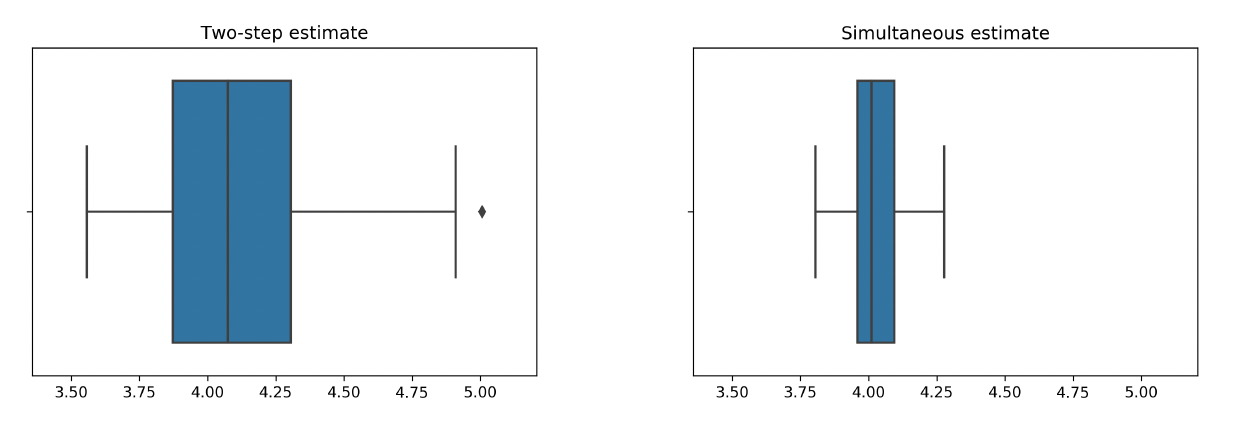
Last, we examine the precision of the estimator for the dispersion parameter $\phi$. Recall that the dispersion parameter is independent of variable selection in the mean regression. To examine the performance, we replicate the experiment 100 times. In each replication, the dispersion parameter is estimated using both the $\chi^2$ statistic and the likelihood-based method. Figure 17 presents the boxplots of the estimates from the two methods. The $\chi^2$ approach is a two-stage estimation and is based on the Pearson residuals; in contrast, the likelihood approach estimates the dispersion and other parameters in the model simultaneously. The relative biases are 0.005 and 0.03, and the nominal standard deviations are 0.1 and 0.33, for the simultaneous and two-stage estimations, respectively. The results suggest that given that the regression function is reasonably approximated, additional model parameters can be consistently estimated. As anticipated, the likelihood-based estimation is more efficient and thus preferred.

Figure 17.Boxplots of estimates of the dispersion parameter from 100 replications. The left and right panels correspond to the two-step and simultaneous estimation respectively.

5. Applications

We use data on health care utilization to illustrate the proposed sparse two-part model. The data are obtained via the Medical Expenditure Panel Survey (MEPS). Conducted by the Agency for Healthcare Research and Quality (a unit of the Department of Health and Human Services), the MEPS consists of a set of large-scale surveys of families and individuals, their medical providers, and employers across the United States. We focus on the household component, which constitutes a nationally representative sample of the U.S. civilian noninstitutionalized population. The data contain records on individuals’ use of medical care, including their use of various types of services and the associated expenditures. In addition, the data set provides detailed information on person-level demographic characteristics, socioeconomic status, health conditions, health insurance coverage, and employment. Using survey data for the years 2008–2011, our study considers a subsample of 74,888 non-elderly adults (of ages ranging between 18 and 64 years).

We examine utilization of hospital outpatient services. For each individual per year, the care utilization is measured by the number of visits and the medical expenditure. The two-part model has been a standard approach to modeling healthcare utilization in the health economics literature (see, for instance, Mullahy 1998 and Shi and Zhang 2015). In this study, we consider the two-part model with dependent frequency and severity. In the frequency component, we employ a Poisson distribution to model the number of hospital outpatient visits. In the severity component, we employ a gamma distribution to model the average medical expenses per visit where the number of visits is used as the weight in the dispersion. Table 2 summarizes the covariates used in the model-building process.

We consider three models for both the frequency component and the average severity component—the linear, deep, and sparse deep two-part models. The linear model uses linear combinations of covariates as the regression function in the Poisson and gamma GLMs. The deep two-part model uses basis functions formed by the feedforward neural networks in the GLMs for the frequency and severity components. The sparse deep two-part model performs covariate selection in the deep learning method. We split the data, using 70% of the data to develop the model and the remaining 30% to evaluate predictive performance. We report the number of data points used to train the alternative models at the bottom of Table 2. In addition, Table 2 identifies the selected covariates for the frequency and severity components in the sparse deep two-part model.

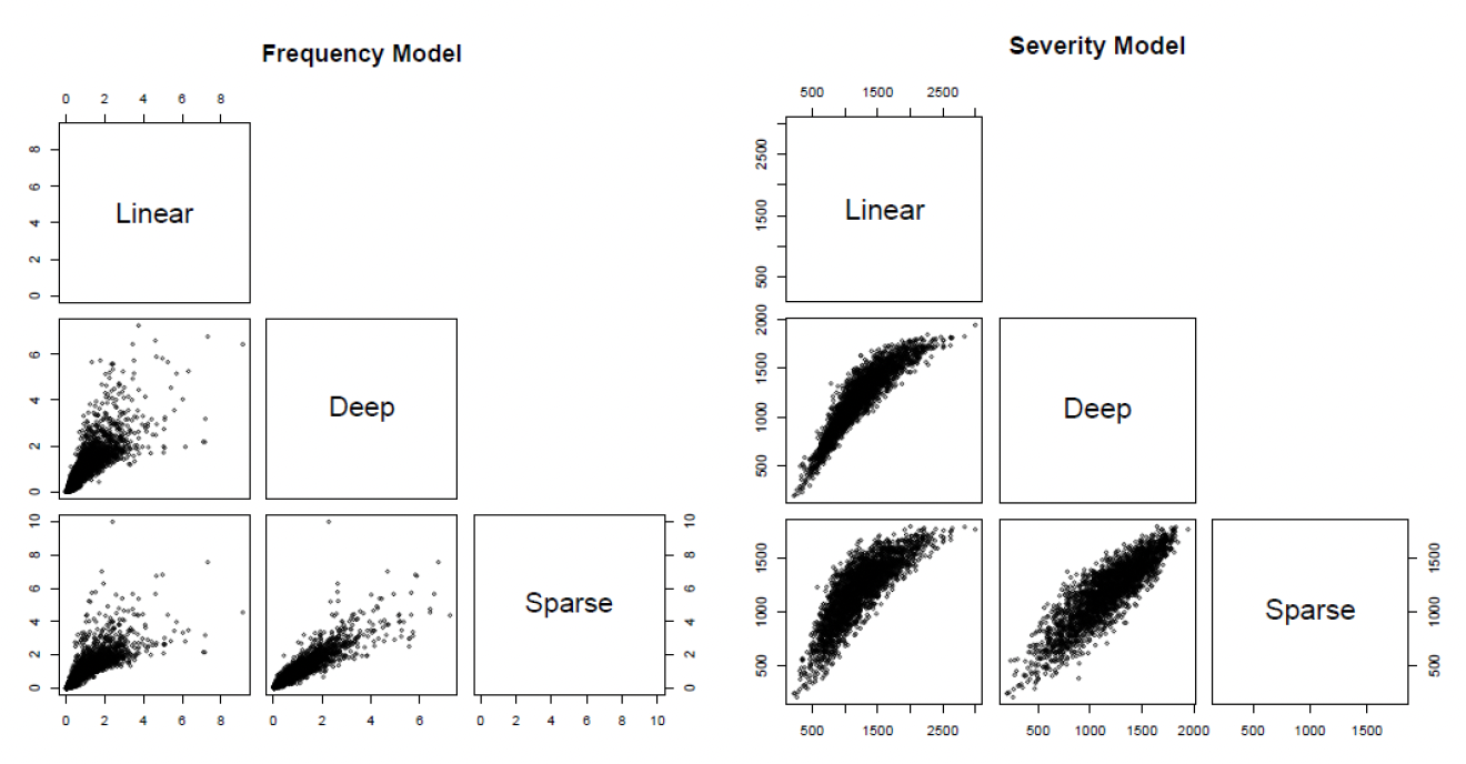
We use the trained models to predict the number of hospital outpatient visits and the average medical expenditure per visit for the observations in the test data. Figure 18 compares the predicted values for the number of hospital outpatient visits and the average medical expenditure from the linear, deep, and sparse deep two-part models. It is not surprising that the predictions from various models are highly correlated because they are based on different estimations for the mean functions in the Poisson and gamma models. However, the differences among various predictions are also noticeable. In particular, the deep learning methods seem to be less susceptible to the extremal observations in the data—hence the corresponding predictions exhibit less variation.

Figure 18.Comparison of predictions from the linear, deep, and sparse deep two-part models. The left and right panels corresponds to frequency and severity components respectively.

Finally, we employ a champion-challenger test based on the Gini index to compare the predictions from various methods. Frees, Meyers, and Cummings (2011) proposed the Gini index to summarize insurance scores. One can relate this practice to the ratemaking application. In the champion-challenger test, we are evaluating whether switching from a base premium to an alternative premium could help the insurer identify profitable business. We report the Gini indices and the associated standard errors in Table 3. The table consists of two parts, one for the frequency outcome and the other for the average severity outcome. For each part, a row in the table considers the prediction from a given method as the base and uses predictions from alternative methods to challenge the base. For instance, the first row assumes that the insurer uses the scores from the linear model as the base, and examines whether risks can be better separated if one switches to the scores from the deep learning methods. The large Gini indices suggest that the scores from both deep learning methods could help the insurer generate more profits. From the pairwise comparisons in the table, we conclude that the proposed deep two-part model outperforms the standard linear two-part model, and variable selection in the deep learning method further improves the prediction.

6. Concluding remarks

In this paper, we propose a sparse deep two-part approach for modeling the joint distribution of claim frequency and average claim severity in the classic two-part model framework. The method employs the basis functions formed by deep feedforward neural networks and thus provides a powerful tool for approximating regression functions with multiple regressors. The frequency-severity model has found extensive use in non-life insurance applications such as ratemaking and portfolio management, which justifies the importance of the proposed work.

Our work’s primary contribution is to introduce a frequency-severity modeling framework that can simultaneously accommodate potential nonlinear covariates’ effects and perform the selection of covariates. Despite the importance of both aspects in actuarial practice, addressing both in a single framework has not been found to be straightforward. We investigate the sparse deep two-part model using extensive numerical experiments and demonstrate its superior performance in real data applications.

In particular, we stress the novelty of variable selection in deep learning methods. We note that although variable selection based on regularization has been extensively studied in the literature of statistical learning, the problem has been somewhat overlooked in the context of neural networks. Our work fills that gap in the literature. We accomplish this through a novel use of group lasso penalties in the model-training process. We discuss the challenges of variable selection for both continuous and categorical covariates.

To illustrate the proposed model’s applicability, we discuss how it relates to ratemaking and how it is applied in practice. Specifically, one assumes a deep Poisson GLM for claim frequency and a deep gamma GLM for claim severity. One obtains the pure premium based on the following steps:

1. For the Poisson model, select important rating variables (both categorical and numeric) following the illustrations in Section 4.1 and Section 4.2.

2. For the gamma model, select important rating variables (both categorical and numeric) following the illustrations in Section 4.3.

3. Calculate the expected number of claims, or the relativity of claim frequency, and the expected claim amount, or the relativity of claim severity. Combining the two components, one obtains the pure premium for a specific risk class.

In conclusion, we would like to highlight a few challenges associated with our method that present promising opportunities for future research. First, although the network-based method exhibits superior predictive accuracy versus the traditional GLM, it is important to acknowledge the trade-off made in terms of interoperability for model parameters. This aspect warrants further investigation and potential refinement to ensure greater flexibility in parameter sharing. Second, it is worth noting that the current method is primarily focused on standard feedforward networks. Exploring the applicability of our approach to other types of networks, such as recurrent or convolutional networks, could prove an intriguing avenue for accommodating diverse types of predictors. Third, we employ categorical embedding to handle discrete predictors within the network. However, in cases where categorical variables possess a natural ordering, such as in territorial ratemaking (Shi and Shi 2017), it becomes crucial to account for such ordering during model fitting. Future investigations should incorporate such considerations to ensure accurate and meaningful representations of ordered categorical predictors.