
1. Introduction
Compositional data describe parts of some whole and are commonly presented as vectors of proportions, percentages, concentrations, or frequencies. The sums of these vectors are constrained to be some fixed constant (e.g., 100%) but can be presented in other forms. Due to such constraints, compositional data possess the following properties (Pawlowsky-Glahn, Egozcue, and Tolosana-Delgado 2015):
Scale invariance. They carry relative rather than absolute information. In other words, the information does not depend on the particular units used to express the compositional data.
Permutation invariance. Permutation of components of a compositional vector does not change the information contained in the compositional vector.
Subcomposition coherence. Information conveyed by a compositional vector of components should not contradict that coming from a subcomposition containing components of the original components.
These properties are important for understanding the consequences that can make the application of conventional statistical methods restrictive and invalid for compositional data.
Consider the case that such data are multivariate observations that carry relative information between components. Applying standard statistical methodology designed for unconstrained data directly to analyze such compositional features can affect inference leading to paradoxes and misinterpretations. Table 1 shows an example of Simpson’s paradox (Pawlowsky-Glahn, Egozcue, and Tolosana-Delgado 2015). Table 1(a) shows the number of students in two classrooms who arrive on time and are late, classified by gender. Table 1(b) shows the corresponding proportions of students arriving on time or being late. Table 1(c) shows the aggregated number of students from the two classrooms who arrive on time and are late. The corresponding proportions are shown in Table 1(d). From Table 1(b), we see that the proportion of female students arriving on time is greater than that of male students in both classrooms. However, Table 1(d) shows the opposite result: the proportion of male students arriving on time is greater than that of female students. The Simpson’s paradox tells us that we need to be careful about inferring from compositional data. The conclusions made from a population may not be true for subpopulations and vice versa.

Our motivation for studying compositional data regression in insurance comes from the fact that there has been a recent explosion of telematics data analysis in insurance (Verbelen, Antonio, and Claeskens 2018; Guillen et al. 2019; Pesantez-Narvaez, Guillen, and Alcañiz 2019; Denuit, Guillen, and Trufin 2019; Guillen et al. 2020; So, Boucher, and Valdez 2021. In telematics data, we typically observe total mileage traveled by an insured during the year and mileage traveled in different conditions such as at night, over speed, or in urban areas. The distances traveled in different conditions are examples of compositional data. However, compositional data do not receive special treatment in some existing actuarial literature. For example, Guillen et al. (2019) and Denuit, Guillen, and Trufin (2019) selected some percentages of distances traveled in different conditions and treated them as ordinary explanatory variables. Pesantez-Narvaez, Guillen, and Alcañiz (2019) treated compositional predictors as ordinary explanatory variables in their study of using XGBoost and logistic regression to predict motor insurance claims with telematics data. Guillen et al. (2020) also treated compositional predictors as ordinary explanatory variables in their negative binomial regression models. Verbelen, Antonio, and Claeskens (2018) used compositional data in generalized additive models and proposed a conditioning and a projection approach to handle structural zeros in components of compositional predictors; this is one of the few studies in insurance that considers handling compositional data. However, the study does not consider dimension-reduction techniques for compositional data in its regression models. Other areas of actuarial science in which compositional techniques previously have been used include capital allocation problems (see Belles-Sampera, Guillen, and Santolino 2016; Boonen, Guillen, and Santolino 2019) and mortality forecasting (see Kjærgaard et al. 2019).
Compositional data analysis dates back to the end of the nineteenth century when Karl Pearson published an article about spurious correlations (Pearson 1897). The classical method for dealing with compositional data is the logratio transformation method, which preserves the aforementioned properties. As pointed out by Atchison (2003), the logratio transformations cannot be applied to compositional data with zeros. In insurance data (e.g., telematics data), components of compositional vectors with zeros can be quite common. This sparsity imposes additional challenges to analyze compositional data in insurance. For more information about compositional data analysis, readers are referred to Aitchison and Egozcue (2005); Pawlowsky-Glahn and Buccianti (2011); and Pawlowsky-Glahn, Egozcue, and Tolosana-Delgado (2015).
In this article, we investigate regression modeling of compositional variables (i.e., covariates) by using the exponential family principal component analysis (EPCA) to learn low-dimensional representations of compositional data. Such representations of the compositional predictors extend the classical principal component analysis (PCA) as well as its probabilistic extension via probabilistic PCA, both of which are special cases of EPCA. See Tipping and Bishop (1999). The contributions of this article are summarized as follows:
-
It brings the issues of compositional data to actuaries’ attention and provides a framework for incorporating compositional data in actuarial models.
-
It presents a detailed case study of compositional data analysis in the insurance context.
-
It produces R code that can be used by practitioners and researchers to replicate the analysis and in their future work.
The remaining part of the paper is organized as follows. In Section 2, we present four negative binomial regression models for fitting the data. In Section 3, we provide numerical results of applying the proposed regression models to a mine injury dataset. In Section 4, we conclude the paper with some remarks.
2. Methods and Models
In this section, we present the models for the compositional data described in the previous section. In particular, we first present the logratio transformation in detail. Then we present a dimension-reduction technique for compositional data. Finally, we present regression models with compositional covariates.
2.1. Methods for compositional data analysis
The classical method for dealing with compositional data is the logratio transformation method, which preserves the aforementioned properties. Let be a compositional data set with compositional vectors. These vectors are assumed to be contained in the simplex
Sd={x∈Rd:d∑j=1xj=κ;∀j,xj>0},
where is a constant, usually 1. The superscript in does not denote the dimensionality of the simplex as the dimensionality of the simplex is
The logratio transformation method transforms the data from the simplex to the real Euclidean space. There are three common types of logratio transformations (Aitchison 1994): centered logratio transformation (CLR), additive logratio transformation (ALR), and isometric logratio transformation (ILR). CLR scales each compositional vector by its geometric mean; ALR applies logratio between a component and a reference component; and ILR uses an orthogonal coordinate system in the simplex.
Let be a column vector (i.e., a vector). CLR is defined as
clr(x)=logxg(x)=log(x)−1dd∑j=1log(xj)=Mclog(x),
where is the geometric mean of and is a matrix. Here is a identity matrix and is a vector of ones, i.e.,
Mc=(10⋯001⋯0⋮⋮⋱⋮00⋯1)−1d(11⋮1)(11⋯1)=(10⋯001⋯0⋮⋮⋱⋮00⋯1)−1d(11⋯111⋯1⋮⋮⋱⋮11⋯1).
ALR is defined similarly. Suppose that the th component of compositional vectors is selected as the reference component. Then ALR is defined as
alr(x)=log(x)−log(xd)==Malog(x),
where is the th component of and is a matrix given by
Ma=(Id−1−1d−1)=(10⋯0−101⋯0−1⋮⋮⋱⋮−100⋯1−1).
ILR involves an orthogonal coordinate system in the simplex and is defined as
ilr(x)=R⋅clr(x),
where is a matrix that satisfies the following conditions:
RRT=Id−1,RTR=Mc=Id−1d1d1Td.
The matrix is called the contrast matrix (Pawlowsky-Glahn, Egozcue, and Tolosana-Delgado 2015). CLR and ILR have the following relationship:
RTilr(x)=RTRclr(x)=RTRRTRlog(x)=RTRlog(x)=clr(x).
Further, we have
Rclr(x)=RRTilr(x)=ilr(x).
All three logratio transformation methods are equivalent up to linear transformations. ALR does not preserve distances. The CLR method preserves distances but can lead to singular covariance matrices. The ILR method avoids these drawbacks.
These logratio transformation methods provide one-to-one mappings between the real Euclidean space and the simplex and allow transforming back to the simplex from the Euclidean space without loss of information. The reverse operation of CLR, for example, is given by
x=clr−1(z)=κexp(z)∑dj=1exp(zj),
where is the transformation of under the CLR method. The reverse operation of ILR is given by
x=clr−1(RTilr(x)),
where is defined in Equation (4).
2.2. PCA for compositional data
In this subsection, we introduce some dimension-reduction methods for compositional data. In particular, we introduce the traditional PCA and the EPCA for compositional data in details. The EPCA methodology has recently been shown to transform compositional data to uncover meaningful structures (Avalos et al. 2018).
The EPCA method is a generalized PCA method for distributions from the exponential family that was proposed and formulated by Collins, Dasgupta, and Schapire (2002) based on the same ideas of generalized linear models. To describe the traditional PCA and the EPCA methods, let us first introduce the -PCA method because both the traditional PCA and the EPCA methods can be derived from the -PCA method.
We consider a data set consisting of numerical vectors, each of which consists of components. For notation purpose, we assume all vectors are column vectors and is a matrix.
Let be a convex and differentiable function. Then the -PCA aims to find matrices and with that minimize the following loss function:
Lφ−PCA(X;A,V)=n∑i=1Dφ(xi,VTai),
where is the th column of and denotes the Bregman divergence:
Dφ(x,y)=φ(x)−φ(y)−(x−y)T[▽φ(y)].
Here denotes the vector differential operator. A Bregman divergence can be thought of as a general distance. Table 2} gives two examples of convex functions and the corresponding Bregman divergences.
For an exponential family distribution, the conditional probability of a value given a parameter value has the following form:
logP(x|θ)=logP0(x)+xθ−G(θ),
where is a function of only, is the natural parameter of the distribution, and is a function of that ensures that is a density function. The negative log-likelihood function of the exponential family can be expressed through a Bregman divergence. To see this, let be a function defined by F(h(θ))+G(θ)=h(θ)θ, where is the derivative of From the above definition, we can show that where Hence,
−logP(x|θ)=−logP0(x)−xθ+G(θ)=−logP0(x)−xθ+h(θ)θ−F(h(θ))=−logP0(x)−F(x)+F(x)−F(h(θ))−(x−h(θ))θ=−logP0(x)−F(x)+F(x)−F(h(θ))−(x−h(θ))f(h(θ))=−logP0(x)−F(x)+φF(x,h(θ)),
which shows that the negative log-likelihood can be written as a Bregman distance plus two terms that are constant with respect to As a result, minimizing the negative log-likelihood function with respect to is equivalent to minimizing the Bregman divergence.
The EPCA method aims to find matrices and with that maximize the following loss function:
LEPCA(X;A,V)=logP(X|A,V)=n∑i=1d∑j=1logP(xji|θji),
where
θji=l∑h=1ahivhj
or
\boldsymbol{\Theta} = (\theta_{ji})_{d\times n} = V^TA.
In other words, the EPCA method seeks to find a lower dimensional subspace of parameter space to approximate the original data. The matrix contains basis vectors of and is represented as a linear combination of the basis vectors. The traditional PCA is a special case of EPCA when the normal distribution is appropriate for the data. In this case,
To apply the traditional PCA to compositional data, we first need to transform them from the simplex into the real Euclidean space by using a logratio transformation method (e.g., the CLR method). When the compositional data are transformed by the CLR method, the traditional PCA has the following loss function:
\mathcal{L}_{PCA}(X;A,V) = \dfrac{1}{2}\Vert\operatorname{clr}(X) - V^TA\Vert^2,\tag{10}
where is the CLR-transformed data.
Avalos et al. (2018) proposed the following EPCA method for compositional data:
\mathcal{L}_{EPCA}(X;A,V) = D_{exp}(\operatorname{clr}(X), V^TA ),\tag{11}
where is the Bregman divergence corresponding to the function. With this setup, we employ an optimization procedure to find and such that the loss function is minimized.
2.3. Regression with compositional covariates
Compositional data in regression models are a set of predictor variables that describes parts of some whole and is commonly presented as vectors of proportions, percentages, concentrations, or frequencies.
Pawlowsky-Glahn, Egozcue, and Tolosana-Delgado (2015) presented a linear regression model with compositional covariates. The linear regression model is formulated as follows:
\hat{y}_i = \beta_0 +\langle \boldsymbol{\beta}, {\bf x}_i\rangle_a,\tag{12}
where is a real intercept and is the Aitchison inner product defined by
\begin{align} \langle \boldsymbol{\beta}, {\bf x}_i\rangle_a &= \langle \operatorname{clr}(\boldsymbol{\beta}), \operatorname{clr}({\bf x}_i)\rangle=\langle \operatorname{ilr}(\boldsymbol{\beta}), \operatorname{ilr}({\bf x}_i)\rangle\\ &=\sum_{j=1}^d \log\dfrac{\beta_j}{g(\boldsymbol{\beta})}\log\dfrac{x_j}{g({\bf x})}. \end{align}
Here denotes the geometric mean. The sum of squared errors is given by
\begin{align} SSE &= \sum_{i=1}^n \left(y_i - \beta_0 - \langle \boldsymbol{\beta}, {\bf x}_i\rangle_a \right)^2 \\ &= \sum_{i=1}^n \left(y_i - \beta_0 - \langle \operatorname{ilr}(\boldsymbol{\beta}), \operatorname{ilr}({\bf x}_i)\rangle \right)^2,\end{align}\tag{13}
which suggests that the actual fitting can be done using the ILR-transformed coordinates, that is, a linear regression can be simply fitted to the response as a linear function of CLR should not be used because it requires the generalized inversion of singular matrices.
Since the response variable of the mine data set is a count variable, it is not suitable to use linear regression models. Instead, we will use generalized linear models to model the count variable. Common generalized linear models for count data include Poisson regression models and negative binomial models (Frees 2009). Poisson models are simple but restrictive as the Poisson distribution has only one parameter. The negative binomial distribution has two parameters. In this study, we use negative binomial models as they provide more flexibility than do Poisson models.
Let denote the predictors from observations. The predictors can be selected in different ways. For example, the predictors can be the ILR-transformed data or the principal components produced by a dimension-reduction method such as the traditional PCA and the EPCA methods. For let be the response corresponding to In a negative binomial regression model, we assume that the response variable follows a negative binomial distribution:
\small{ P(y=j) = \dfrac{\Gamma(j+r)}{j!\Gamma(r)} p^r (1-p)^j,\quad j=0,1,2,\ldots,\tag{14}}
where and are parameters and denotes the gamma function. The mean and the variance of a variable are given by
E[y] = \frac{r(1-p)}{p},\quad \operatorname{Var}{(y)} = \frac{r(1-p)}{p^2}.
To incorporate covariates in a negative binomial regression model, we let the parameter vary by observation. In particular, we incorporate the covariates as follows:
\mu_i = \frac{r(1-p_i)}{p_i} = E_i \exp\left({\bf x}_i'\boldsymbol{\beta}\right),\tag{15}
where and are parameters to be estimated and is the exposure. For the mine data set, we use the variable AVG_EMP_TOTAL as the exposure. This is similar to modeling the number of claims in a Property and Casualty data set where the time to maturity of an auto insurance policy is used as the exposure (Frees 2009; Gan and Valdez 2018). The method of maximum likelihood can be used to estimate the parameters.
In this study, we compare four negative binomial models. Table 3 describes the covariates of the four models. In the first model, we use the original compositional components as the covariates. Since the sum of the compositional components is equal to 1, we exclude the first component in the regression model to avoid overparameterization. In the second model, we use the compositional components transformed by the ILR method that is defined in Equation (3). In the third model, we use the first few principal components obtained from the traditional PCA method that is defined in Equation (10). In the fourth model, we use the first few principal components obtained from the EPCA method that is defined in Equation (11).
2.4. Validation measure
To measure the accuracy of regression models for count variables, it is common to use Pearson’s chi-square statistic, which is defined as
\chi^2 = \sum_{j=0}^{m} \frac{ (O_j - E_j)^2 }{E_j},\tag{16}
where is the observed number of mines that have injuries, is the predicted number of mines that have injuries, and is the maximum number of injuries considered over all mines. Between two models, we prefer the model with a lower chi-square statistic.
The observed number of mines that have injuries is obtained by
O_j = \sum_{i=1}^n I_{\{y_i=j\}}, \quad j=0,1,\ldots,m,
where is an indicator function. The predicted number of mines that have injuries is calculated as follows:
\begin{aligned} E_j &= E\left[ \sum_{i=1}^n I_{\{\hat{y}_i=j\}} \right] = \sum_{i=1}^n E[I_{\{\hat{y}_i=j\}}] = \sum_{i=1}^n P(\hat{y}_i=j) \\ &= \sum_{i=1}^n \dfrac{\Gamma(j+\hat{r})}{j!\Gamma(\hat{r})} \hat{p}_i^{\hat{r}} (1-\hat{p}_i)^j, \end{aligned}
where and are estimated values of the parameters.
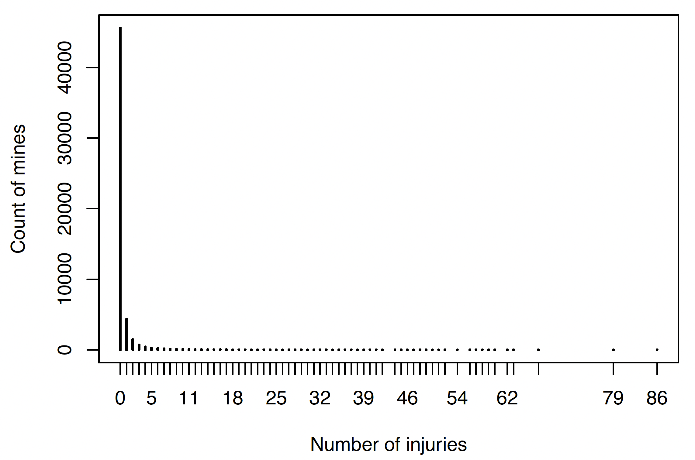
From Figure 2, we see that the maximum observed number of injuries is 86. To calculate the validation measure, we use that is, we use the first 100 terms of s and s. The remaining terms are too close to zero and will be ignored.

In addition to the chi-square statistic, we compare the average observed number of injuries and the predicted number of injuries. To do that, we use the following mean prediction error:
ME = \dfrac{1}{n} \sum_{i=1}^n \left( y_i - \hat{y}_i\right),\tag{17}
where is the number of observations, denotes the observed number of injuries in the th mine, and denotes the predicted number of injuries in the th mine. Between two models, we prefer the model with a lower absolute value of the mean prediction error.
3. Data analysis
In this section, we demonstrate the performance of the models described in the previous section to a mine injury data set obtained from the Internet. Although our research was motivated by telematics data, we do not have access to real telematics data. As a result, we use this mine injury data set to showcase the application of compositional data analysis in actuarial science and insurance.
3.1. Description of the data
We use a data set from the U.S. Mine Safety and Health Administration from 2013 to 2016. The data set was used in the Predictive Analytics exam administered by the Society of Actuaries in December 2018.[1] This data set contains 53,746 observations described by 20 variables, including compositional variables. Table 4 shows the 20 variables and their descriptions. Among the 20 variables, 10 of them (i.e., the proportion of employee hours in different categories) are compositional components.
In our study, we ignore the following variables: YEAR, US_STATE, COMMODITY, PRIMARY, SEAM_HEIGHT, MINE_STATUS, and EMP_HRS_TOTAL. We do not use YEAR in our regression models as we do not study the temporal effect of the data. However, we use YEAR to split the data into a training set and a test set. The variables COMMODITY, PRIMARY, and SEAM_HEIGHT are related to the variable TYPE_OF_MINE, which we will use in our models. The variable EMP_HRS_TOTAL is highly correlated to the variable AVG_EMP_TOTAL, with a correlation coefficient of 0.9942. We use only one of them in our models.
Table 5 shows summary statistics of the categorical variable TYPE_OF_MINE. We also show the number of observations in different years. From the table, we see that there are approximately the same number of observations from different years and that most mines are sand and gravel as well as surface mines.
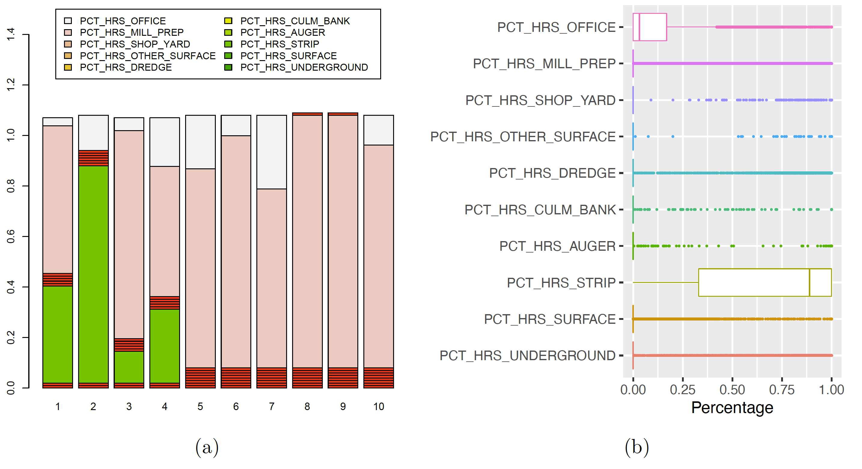
Table 6 shows some summary statistics of the numerical variables. From the table, we see that the average number of employee ranges from 1 to 3115. The compositional components are those variables that start with PCT; each component refers to the proportion of employee hours spent in various types or methods of mining work such as stripping and auger mining. In the data, all compositional components contain zeros. In additional, most compositional components are skewed as the 3rd quantiles are zero. Table 7 shows the percentages of zeros of the compositional variables. From the table, we see that most values of many compositional variables are just zeros.
Figure 1(a) shows the proportions of employee hours in different categories from the first ten observations. Figure 1(b) shows the boxplots of the compositional variables. From the figures, we also see that the compositional variables have many zero values. Zeros in compositional data are irregular values. Pawlowsky-Glahn, Egozcue, and Tolosana-Delgado (2015) discussed several strategies to handle such irregular values. One strategy is to replace zeros by small positive values. In the mine dataset, we can treat zeros as rounded zeros below a detection limit. In this paper, we replace zero components with 10−6, which corresponds to a detection limit of one hour among one million employee hours.

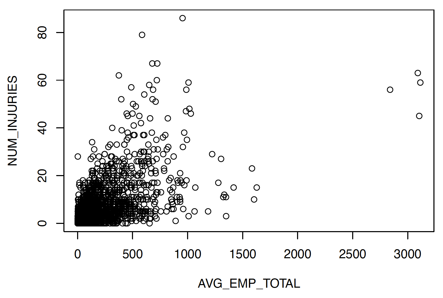
The response variable is the total number of injuries reported. Figure 2 shows a frequency distribution of the response variable. The summary statistics given in Table 6 and Figure 2 show that the response variable is also highly skewed with many zeros. Figure 3 shows a scatter plot between the variable AVG_EMP_TOTAL and the response variable NUM_INJURIES. From the figure, we see that the two variables have a positive relationship. In our models, we will use the variable AVG_EMP_TOTAL as the exposure.

3.2. Results
In this subsection, we present the results of fitting the four negative binomial regression models (see Table 3) to the mine data set. We follow the following procedure to fit and test the models NBILR, NBPCA, and NBEPCA:
-
Replace zeros with small positive values (i.e.,
-
Transform the compositional variables for the whole mine data set. For the model NBILR, we transform the compositional variables with the ILR method. For the model NBPCA, we first transform the compositional variables with the CLR method and then apply the standard PCA to the transformed data. Both the ILR method and the CLR method are available in the R package
compositions. For the model NBEPCA, we transform the compositional variable with the EPCA method implemented by Avalos et al. (2018).[2] -
Split the transformed data into a training set and a test set. In particular, we use data from 2013 to 2015 as the training data and use data from 2016 as the test data.
-
Estimate parameters based on the training set.
-
Make predictions for the test set and calculate the out-of-sample validation measures.
We follow similar procedures to fit and test the model NB except that we do not transform the compositional variables.
We fitted the four models described in Table 3 to the mine dataset according to the afore-mentioned procedure. Table 8 shows the in-sample and out-of-sample chi-square statistics, as well as the mean prediction error (ME), produced by the four models. From the table, we see that the negative binomial model with EPCA transformed data performs the best among the four models. The model NBEPCA produced the lowest chi-square statistics for both the training data and the test data. A similar conclusion can be drawn based on the mean prediction error.
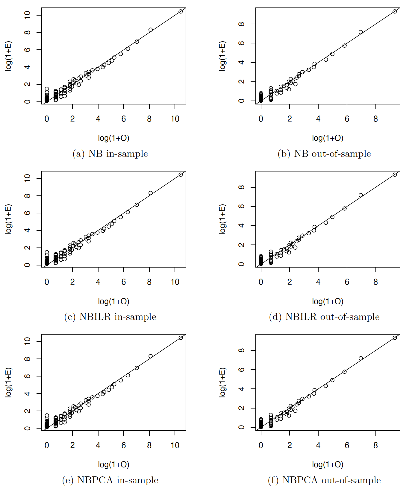
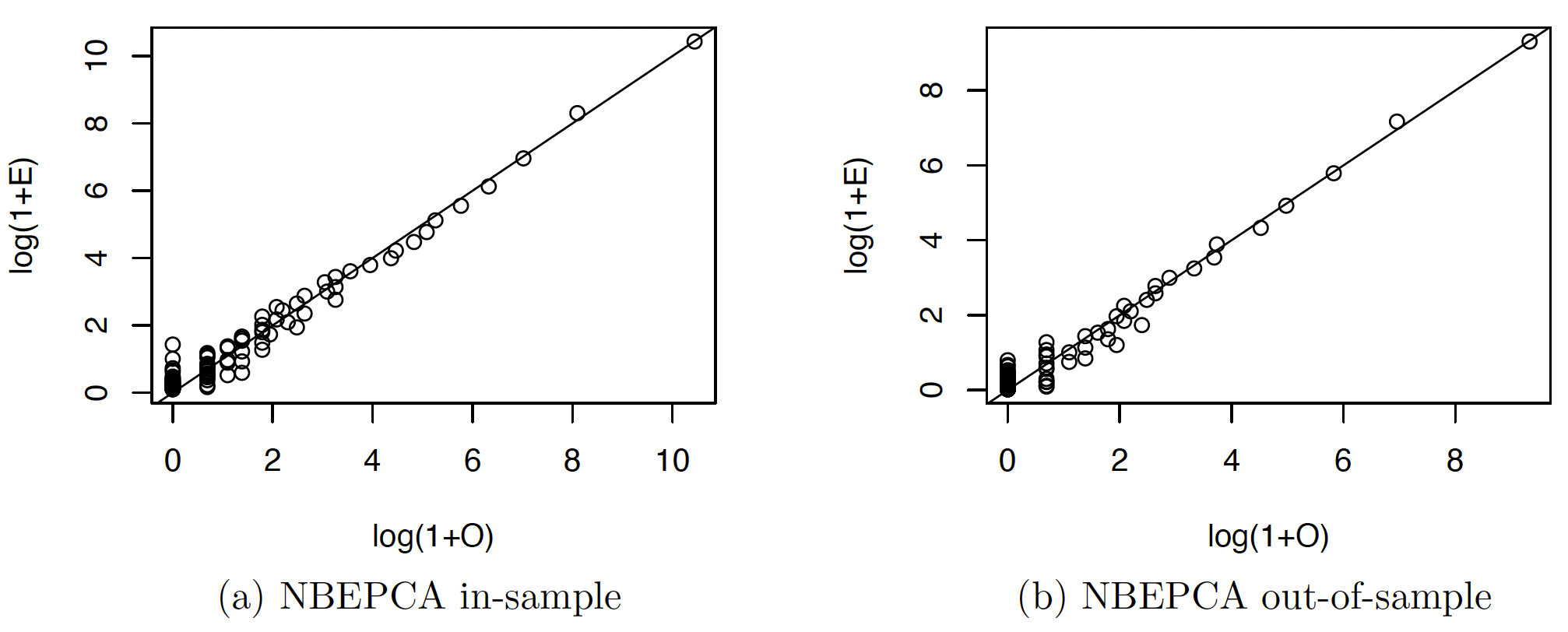
Figure 4 and Figure 5 show the scatter plots of the observed number of mines with different number of injuries and that predicted by the models at scales. That is, the scatter plots show the relationship between and for We use scale here because the 's and 's have big differences for different 's. From the scatter plots, we see that all the models predict the number of mines with different number of injuries quite well. We cannot tell the differences of the four models from the scatter plots. However, the chi-square statistics shown in Table 8 numerically demonstrates the superiority of the NBEPCA model.


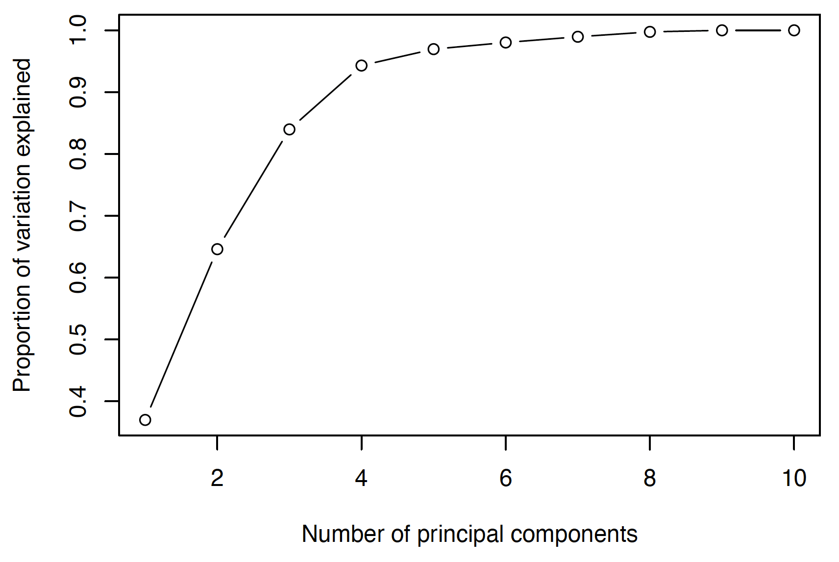
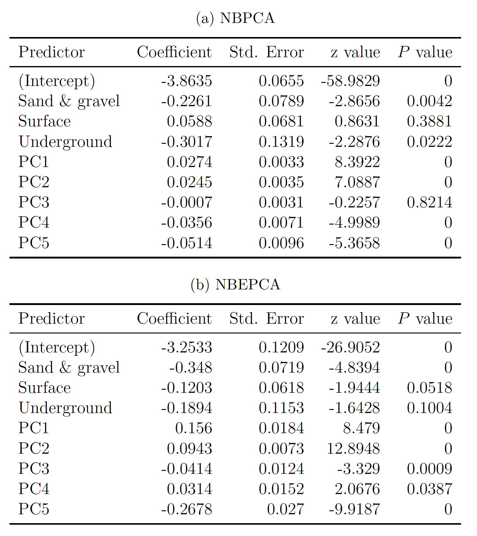
For the NBPCA model, we selected the first five principal components produced by applying the standard PCA to the CLR-transformed data. Figure 6 shows the proportion of variation explained by different numbers of principal components. The first five principal components can explain more than 95% of the variation of the original data. For the NBEPCA model, we selected the first five principal components for the same reason. The EPCA method used to transform the compositional variables is slow and took a normal desktop about 20 minutes to finish the computation. The reason is that the EPCA method we used is implemented in R, which is a scripting language that may not be efficient for iterative optimization.

Table 9 shows the estimated regression coefficients of the model NB. In this model, we used the original compositional variables by assuming that these variables contain absolute information. Since the sum of the compositional variables equals 1, we excluded the first compositional variable to avoid overparameterization. Table 9 shows the estimated regression coefficients for the nine compositional variables. The P values of these coefficients show that all the compositional variables are statistically significant.
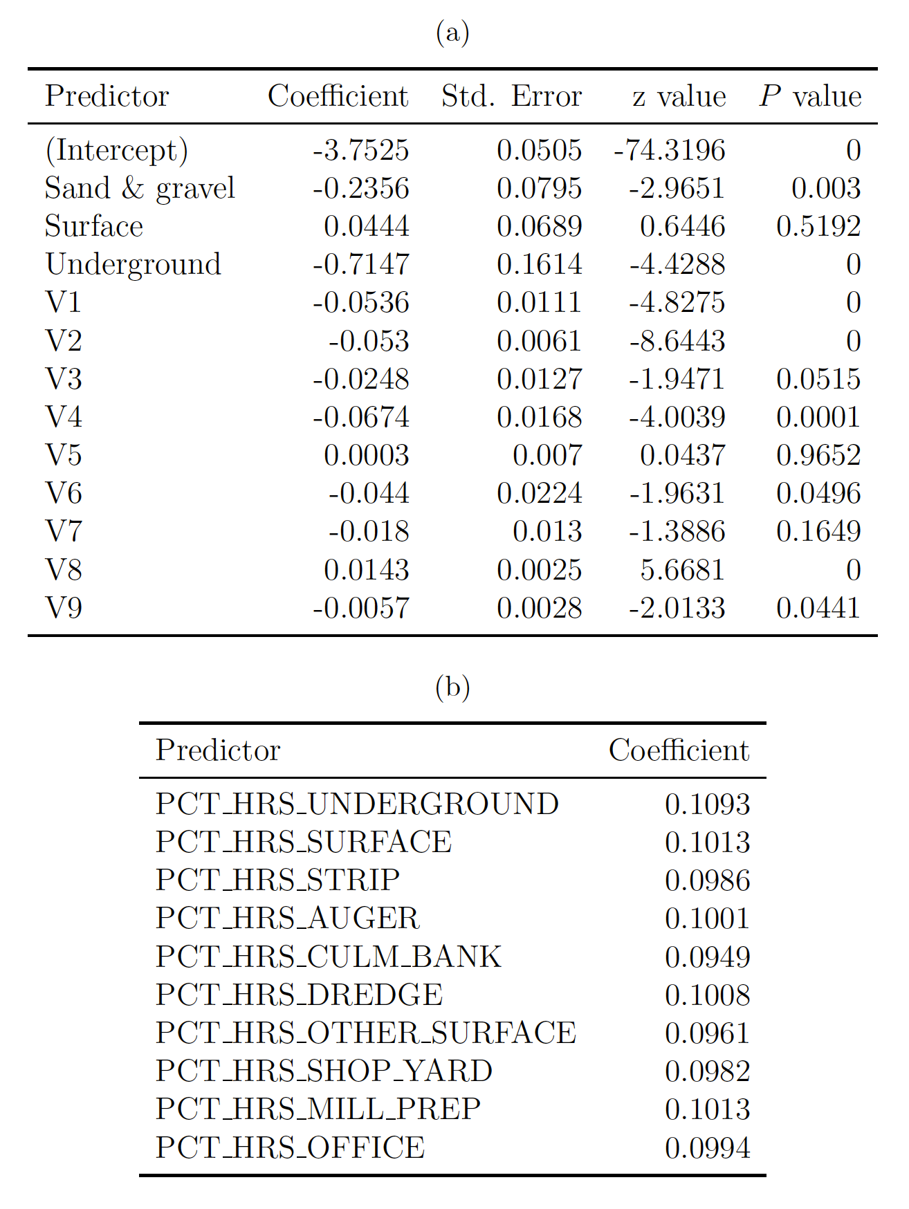
Table 10 shows the estimated regression coefficients of the model NBILR. As shown: in Table 10(a), the ten compositional variables are transformed to nine variables by the ILR method. Table 10(b) shows the regression coefficients transformed back to the CLR proportions by the inverse operation of the ILR method. From Table 10(b), we see that the coefficients of the ten compositional variables are similar and are quite different from the coefficients of the ILR variables to From the values shown in Table 10(a), we see that some of the ILR transformed variables are not significant. For example, the variable V5 has a value of 0.9652 and the variable has a value of 0.1649 . Both variables have a value greater than 0.1 . This suggests that it is appropriate to reduce the dimensionality of the compositional variables.
_shows_the_coefficients_of_.png)
The regression coefficients of the ILR transformed variables to shown in Table 10 vary a lot. It is challenging to interpret those coefficients. From the values shown in Table 10(a), we see that some of the ILR transformed variables are not significant. For example, the variable V5 has a value of 0.9652 and the variable V7 has a value of 0.1649 . Both variables have a value greater than 0.1. This suggests that it is appropriate to reduce the dimensionality of the compositional variables.
Table 11 shows the estimated regression coefficients of the models NBPCA and NBEPCA. We used five principal components in both models. From Table 11(b), we see that all principal components produced by the EPCA method are significant. However, Table 11(a) shows that the third principal component PC3 produced by the traditional PCA method is not significant as it has a value of 0.8214.

In summary, our numerical results show that the EPCA method is able to produce better principal components than the traditional PCA method and that using the principal components produced by the EPCA method can improve the prediction accuracy of the negative binomial models with compositional covariates.
4. Conclusions
It is important to recognize the unique aspects of compositional data when using and fitting them as feature variables in predictive models. Compositional data are commonly presented as vectors of proportions, percentages, concentrations, or frequencies. A peculiarity of these vectors is that their sum is constrained to be some fixed constant, e.g., 100%. Due to such constraints, compositional data have the following properties: they carry relative information (scale invariance); equivalent results should be yielded when the ordering of the parts in the composition is changed (permutation invariance); and results should remain consistent if a noninformative part is removed (subcomposition coherence).
In this article, we offer methods to handle regression models with compositional covariates using a mine data set for empirical investigation. We built negative binomial regression models to predict the number of injuries from different mines. In particular, we built four negative binomial regression models: a model with the original compositional components, a model with ILR-transformed compositional variables, a model with principal components produced by the traditional PCA, and a model with principal components produced by the EPCA. Our numerical results show that the EPCA method for controlling compositional covariates produces principal components that are significant predictors and improve the prediction accuracy of the regression model. However, the EPCA method may unavoidably have some limitations. For example, interpreting the regression coefficients is not straightforward due to the transformation. In addition, the log transformation requires dealing with zeros in the data.
The data set is available at https://www.soa.org/globalassets/assets/files/edu/2018/2018-12-exam-pa-data-file.zip.
The R code of the EPCA method is available at https://github.com/sistm/CoDa-PCA.