A Cost-of-Capital Risk Margin Formula for Nonlife Insurance Liabilities

1. Introduction

With the growing influence of Bayesian Markov chain Monte Carlo (MCMC) models in stochastic loss reserving (e.g., Meyers 2015), this paper will illustrate one way to use such a model to calculate a cost-of-capital risk margin for nonlife insurance liabilities. The need for such a calculation is found in the “technical provisions” specified in the European Union’s Solvency II act.^[1]

Those technical provisions refer to the insurer’s liability for unpaid losses. Specifically:

1. “The value of the technical provisions shall be equal to the sum of a best estimate and a risk margin.”

2. “The best estimate shall correspond to the probability-weighted average of future cash flows, taking account of the time value of money using the relevant risk-free interest rate term structure.”

3. “The risk margin shall be calculated by determining the cost of providing an amount of eligible own funds equal to the Solvency Capital Requirement necessary to support the insurance obligations over the lifetime thereof.”

4. “Insurance undertakings shall segment their insurance obligations into homogeneous risk groups, and as a minimum by lines of business, when calculating the technical provisions.”

This paper illustrates a way to implement the principles expressed in the above provisions of the act. Although the act goes on to provide some specific provisions on how to implement those principles, the purpose of this paper is more to show how to implement the principles underlying Solvency II using more theoretically sound risk management principles along with the Bayesian MCMC technology. In the concluding remarks, we describe the main differences between the approach in this paper and that specified by Solvency II.

A Bayesian MCMC stochastic loss reserve model provides an arbitrarily large number (say 10,000) of equally likely parameter sets that enable one to simulate future cash flows of the liability. From those parameter sets, it is possible to describe any future state in the model’s time horizon including those states necessary to calculate the technical provisions. That is what this paper will do.

Here is a high-level description of that cash flow:

1. At the end of the current calendar year (call this time t = 0), the insurer posts its best estimate of the liability. The insurer also posts the amount of capital, C₀, needed to contain the uncertainty in this estimate. It invests C₀ in a fund that earns income at the risk-free interest rate i.

2. At the end of the next calendar year, at time t = 1, the insurer uses its next year of loss experience to reevaluate its liability.^[2] It then posts its updated estimate of the liability and the capital, C₁, needed to contain the uncertainty in this estimate. The difference between C₀ • (1 + i) and C₁ is returned to the investor. If that difference is negative, as it occasionally will be, the investor is expected to contribute an amount to make up that difference.

3. The process continues for future calendar years, t, with the amount,

   $$C_{t-1} \cdot(1+i)-C_{t},$$

   being returned to (or being contributed by) the investor.

4. At some time t = u, the loss is deemed to be at the ultimate—that is, no significant changes in the loss are anticipated—and so we set C_t = 0 for t > u. For the examples in this paper, u = 9.

The present value, discounted at the risky rate r, of the amount returned is equal to

$$\sum_{t=1}^{u+1} \frac{C_{t-1} \cdot(1+i)-C_{t}}{(1+r)^{t}} \text {. }$$

Since r > i, this present value will be less than the initial capital investment of C₀. To adequately compensate the investor for taking on the risk of insuring policyholder losses, the difference can be made up at time t = 0 by what we now define as the cost-of-capital risk margin, R_COC:

$$\begin{aligned} R_{C O C} & \equiv C_{0}-\sum_{t=1}^{u+1} \frac{C_{t-1} \cdot(1+i)-C_{t}}{(1+r)^{t}} \\ & =(r-i) \cdot \sum_{t=0}^{u} \frac{C_{t}}{(1+r)^{t+1}} \end{aligned} \tag{1}$$

with the second equality coming after some algebraic manipulations.^[3]

The problem that now needs to be addressed is the calculation of the $C_{t}s$. A straightforward way to project a future cash flow for this process would be to take a fitted Bayesian MCMC model and simulate an additional calendar year of losses for t = 1. Then fit another Bayesian MCMC model to the original data and the simulated data to get the loss estimate and capital requirements for t = 1. Then continue this process for t = 2, . . . , u.

While the execution speed of Bayesian MCMC software has significantly increased in recent years, repeating this for 10,000 simulated future cash flows would undoubtedly strain the patience of most practicing actuaries. This paper will propose a faster way to simulate the future cash flows to calculate the capital requirements for this process.

Now that we have defined the cost-of-capital risk margin, here is the route we will take to address the problems we must solve to calculate the risk margin:

• First we show how to use the Bayesian MCMC machinery to calculate the cash flows and corresponding loss estimates implied by the model.

• Then we show how to calculate the best estimate and the risk margins from the cash flows.

• Then we investigate the effect of insurer size and line of business on risk margins.

• Then we address the effect of diversification by line of business.

Whereas the examples in this paper focus on an “ultimate” time horizon, jurisdictions such as the European Union require insurers to calculate their capital requirements based on a one-year time horizon. The final section shows, with an example, how to adjust the models so that the one-year time horizon can be incorporated within the framework of this paper.

The data for the examples in this paper are taken from the Casualty Actuarial Society (CAS) Loss Reserve Database. The data consist of 50 loss triangles in the commercial auto (CA), personal auto (PA), workers’ compensation (WC), and other liability (OL) lines of insurance. The loss triangles used in this paper were selected from the list given in Appendix A of Meyers (2015).

The algorithms described in this paper are computationally intensive. The reader of this paper might question whether the computations can be done in a reasonable time. The answer is yes. The scripts that are included with the paper were run on the author’s standard issue laptop. The run times for the calculations are about two minutes per loss triangle for the model in Section 3 and about 17 minutes per triangle for the model in Section 5.

2. Cash flows and statistics of interest

This paper uses the changing settlement rate (CSR) model described in Meyers (2015) as modified in Meyers (2018). As those papers show, the model has been successfully validated on the lower triangle holdout data for a set of 200 loss triangles, 50 from each of four lines of business. The model describes the distribution of outcomes $X_{w, d} \sim \operatorname{lognormal}\left(\mu_{w, d}, \sigma_d\right)$, where the accident year w = 1, . . . , 10 and the development year d = 1, . . . , 11 − w. It is fit to a cumulative paid loss triangle, T₀ ≡ {X_w,d}. This model allows for accident year effects, development year effects, and a variable claim settlement rate. The details of the model can be found in Section 3 of Meyers (2018). What is relevant for this paper is that given the loss triangle, T₀, the model uses Bayesian MCMC to obtain a sample of 10,000 equally likely lognormal, $\left\{\mu_{w, d}^j, \sigma_d^j\right\}_{j=1}^{10,000}$, parameter sets from the posterior distribution, $\left\{\mu_{w, d}, \sigma_d \mid T_0\right\}$. This paper uses these parameter sets to describe the possible future cash flows by a simulation.

With these parameter sets we can calculate the best estimate of the liability, as specified by Solvency II, as the probability weighted average of the present value of expected future cash flows. This will be equal to the expected value of the differences in the cumulative payments between development years—that is,

$$\begin{aligned} \sum_{j=1}^{10,000} \sum_{w=2}^{10} \sum_{d=12-w}^{10} \exp \left(\mu_{w, d}^{j}+\left(\sigma_{d}^{j}\right)^{2} / 2\right) \\ E_{\text {Best }}=\frac{\exp \left(\mu_{w, d-1}^{j}+\left(\sigma_{d-1}^{j}\right)^{2} / 2\right)}{10,000 \cdot(1+i)^{w+d-11.5}} \end{aligned} \tag{2}$$

This calculation assumes that the losses are paid one-half year before the end of future calendar year t = w + d − 11.

For the scope of this paper, let’s also select the ultimate loss, U_j, associated with the jth parameter set to be the sum of the expected values of the losses for d = 10 over all the accident years—that is,

$$U_{j}=\sum_{w=1}^{10} \exp \left(\mu_{w, 10}^{j}+\left(\sigma_{10}^{j}\right)^{2} / 2\right) \tag{3}$$

For those wishing to allow for loss development after d = 10, we suggest that a Bayesian MCMC version of Clark (2003) would be a good place to begin.

For the lower triangle of $\left\{X_{w, d}^j\right\}_{j=1}^{10,000}$, define the simulated loss trapezoid for future calendar year t that includes the upper loss triangle, T₀, and the first t diagonals of the lower loss triangle—that is,

$$T_{t}^{j} \equiv\left\{\begin{array}{ll} X_{w, d} & \text { for } w=1, \ldots, 10 \text { and } d=1, \ldots, 11-w \\ X_{w, d}^{j} & \text { for } w=t+1, \ldots, 10 \text { and } \\ & d=12-w, \ldots, \min (11-w+t, 10) \end{array}\right. \tag{4}$$

where $X_{w, d}^j$ is simulated from a lognormal distribution with parameters $\mu_{w, d}^j$ and $\sigma_d^j$.

Let’s temporarily drop the assumption that we know the parameter set index j. All we have is an observed loss trapezoid, T_t. Then using Bayes’ theorem and the fact that, initially, all j are equally likely, the probability that the parameter set index is equal to j given T_t, for t > 0, is given by

$$\operatorname{Pr}\left[J=j \mid T_{t}\right]=\frac{\prod_{X_{w, d} \in \boxminus_{t}} \phi\left(\log \left(X_{w, d}\right) \mid \mu_{w, d}^{j} \sigma_{d}^{j}\right)}{\sum_{k=1}^{10,00} \prod_{X_{w, d} \in \in_{t}} \phi\left(\log \left(X_{w, d}\right) \mid \mu_{w, d}^{k} \sigma_{d}^{k}\right)} \tag{5}$$

where $\phi$ is the probability density function for the normal distribution.

At this point, one can choose from a number of options to calculate the various statistics that are of interest to insurer risk managers. For example, given T_t, one could calculate the ultimate loss estimate, E_t, as

$$E_{t} \equiv E\left[\sum_{w=1}^{10} X_{w, 10} \mid T_{t}\right]=\sum_{j=1}^{10,000} \operatorname{Pr}\left[J=j \mid T_{t}\right] \cdot U_{j} \tag{6}$$

If one accepts that the Bayesian MCMC output is representative of all future scenarios, Equation 6 is exactly the right calculation for the loss estimate given T_t. But let’s consider what one should do to calculate, say, the 99.5th percentile. First one should sort the scenarios in order of increasing U_j. It is not uncommon to find a case where there is a scenario, j, with Pr[J ≤ jT₉] = 0.9900 and Pr[J ≤ j + 1T₉] = 0.9960.

To deal with this, we decided to calculate the statistics of interest by first taking a random sample of size 10,000 (with replacement), {S_t}, of the $U_{j}$s with sampling probabilities Pr[J = jT_t]. It was quite easy to implement and surprisingly fast in R. This is subject to an additional simulation error, but it should be small.

The statistics of interest for risk margin are, for t = 0, . . . , 9,

• the mean, E_t, which is equal to the arithmetic average of {S_t}; and

• the tail value at risk at the α level (TVaR@α), which is equal to the arithmetic average of the (1 − α) • 10,000 highest values of {S_t}.^[4]

Let’s denote the total required capital by C_t ≡ TVaR@α − E_t.

We summarize the above in Algorithm 1.

Algorithm 1.Calculate capital scenarios

The examples in this paper use α = 97%. This selection is for illustrative purposes only.

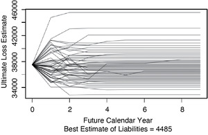
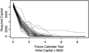
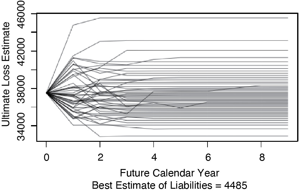
Calculating E_t^k for t = 0, . . . , 9 yields the kth path that the loss estimate takes as it moves toward its ultimate value. Of interest for what follows is the set of possible paths that the loss estimate can take. Figure 2.1 shows those paths that contain the 100th, the 300th, . . . , and the 9,900th highest $E_9^k$s of Insurer #353 for commercial auto in the CAS Loss Reserve Database. This figure illustrates that the $E_t^k$s tend to become more certain over time.

Figure 2.1.Paths of ultimate loss estimates

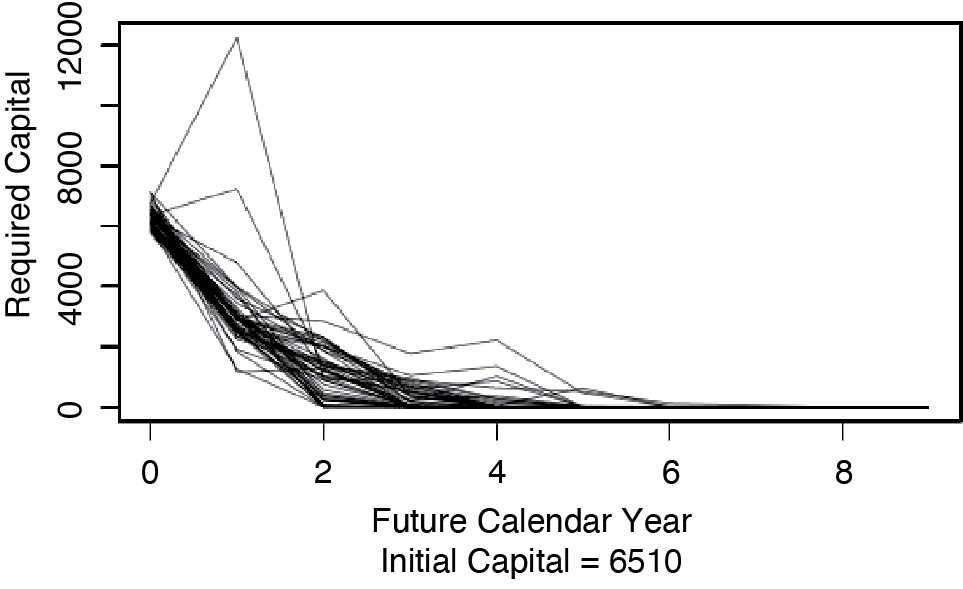
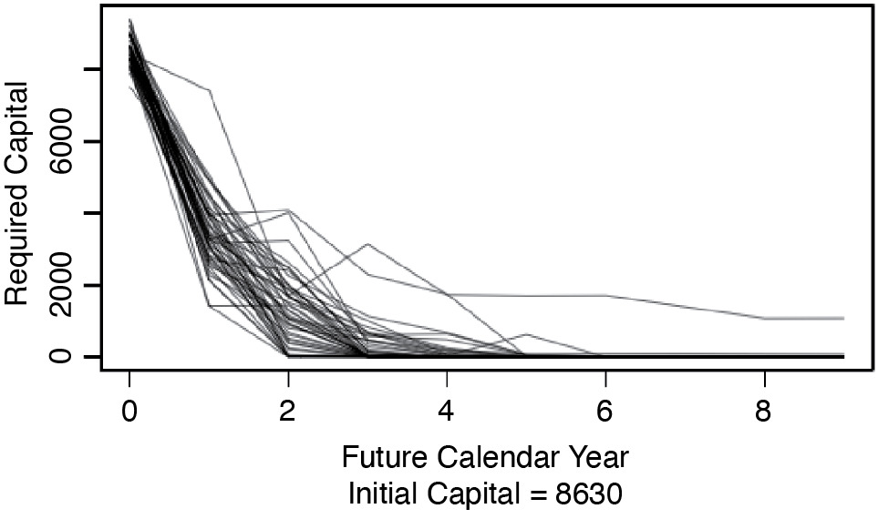
Also of interest are the paths of the required capital, C_t^k, for t = 0, . . . , 9. Figure 2.2 shows the paths of C_t^k that correspond to the paths taken by E_t^k in Figure 2.1. This figure illustrates that as the estimates of the $E_t^k$s become more certain, the required capital, C_t^k, tends to decrease over time.

Figure 2.2.Required capital by calendar year

3. Risk margins

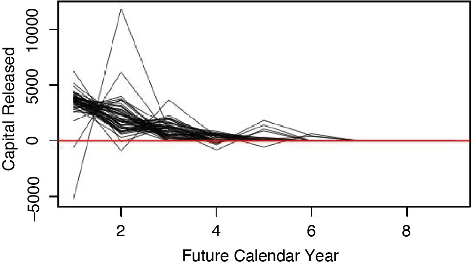
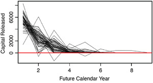
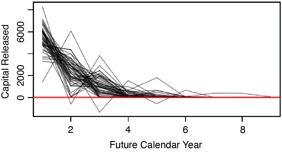
This section applies the cost-of-capital risk margin formula given by Equation 1 to the set of required capital paths, $\left\{C_0^k, \ldots, C_9^k\right\}_{k=1}^{10,000}$. Recall that the formula defined the cost-of-capital risk margin as the present value of the capital released as the loss reserve liability becomes more certain. Figure 3.1 shows the paths of released capital that correspond to the paths taken by the $C_t^k$s in Figure 2.2. In general, this figure shows that most of the capital gets released early on, and that occasionally it is necessary to add capital.

Figure 3.1.Paths of released capital

Applying Equation 1 we get for each k

$$R_{C O C}^{k} \equiv C_{0}^{k}-\sum_{t=1}^{u} \frac{C_{t-1}^{k} \cdot(1+i)-C_{t}^{k}}{(1+r)^{t}} \tag{7}$$

Then the risk margin is given by

$$R_{C O C}=\frac{1}{10,000} \sum_{k=1}^{10,000} R_{C O C}^{k} \tag{8}$$

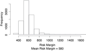
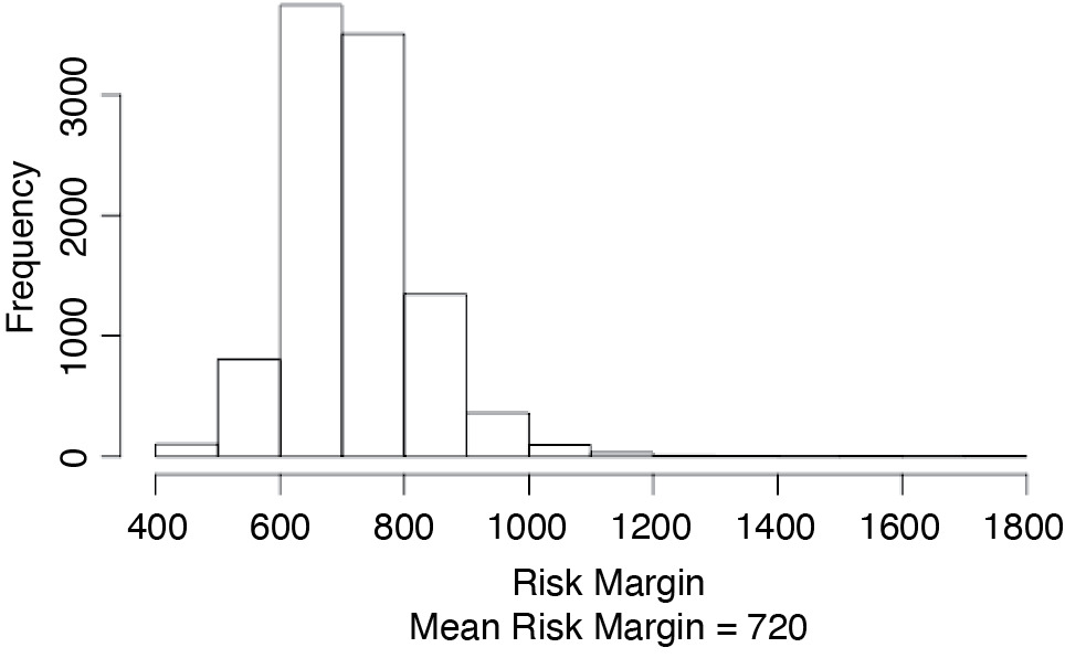
Figure 3.2 shows a histogram of the $R^k_{COC}$s for our example.

Figure 3.2.Risk margin

Of interest is the ratio of the risk margin and the size of the best estimate. To investigate, we calculated the risk margins for all 200 loss triangles in our data. After some exploratory analysis, we concluded that (1) significant differences exist by line of business; and (2) there is an approximate linear relationship between the log of the risk margin and the log of the best estimate. Figure 3.3 shows the plots of the log(R_COC) against log(E_Best), along with the coefficients, along with their standard errors, of an ordinary linear regression of the form

$$\log \left(R_{C O C}\right)=a+b \cdot \log \left(E_{\text {Best }}\right) \tag{9}$$

Figure 3.3.log(Risk Margin) vs. log(Best Estimate)^[5]

We can rewrite Equation 9 in the form

$$\frac{R_{\text {COC }}}{E_{\text {Best }}}=e^{a} \cdot\left(E_{\text {Best }}\right)^{b-1} \tag{10}$$

Note from Figure 3.3 that b 1 for all four lines of insurance. This implies that the risk margin–to–best estimate ratio decreases as the best estimate increases. As Figure 3.4 shows, the ratio can be quite high for insurers with small best estimates. It is easy to see where some insurers might object, especially if the line with the high ratio is a small part of the insurer’s book of business.

Figure 3.4.Risk margin ratio vs. best estimate^[6]

4. Diversification

As noted in the introduction, one provision of the European Union Solvency II act says explicitly, “Insurance undertakings shall segment their insurance obligations into homogeneous risk groups, and as a minimum by lines of business, when calculating the technical provisions.” This means that the total risk margin for a multiline insurer is the sum of the risk margins over its individual lines of business.

Longtime observers of the insurance business have recognized that multiline insurers benefit from the diversification of their risk of loss. This being the case, they might well want to reflect the benefits of diversification in their risk margins. The problem with a formal recognition of diversification is that the benefits have been difficult to quantify. What many are afraid of is the possibility that significant losses from the different lines of business could happen at the same time. This possibility is often referred to as the “dependency problem.”

As such, the Solvency II nonrecognition of diversification may appear to some to be prudent.

Mathematical tools that can be used to describe dependency have been available for quite some time. See, for example, Frees and Valdez (1998) and Wang (1998). The main tool described in those papers is called a copula, which is a multivariate distribution on an L-dimensional unit hypercube in which the marginal distributions have a uniform (0,1) distribution. Given a copula and samples {_lS_t^k} (see Section 2), for each line l of L lines of business one begins to calculate R_COC by first executing Algorithm 2.

Algorithm 2.Calculate samples for dependent lines

Use the output of this algorithm to calculate $\left\{\mathstrut_{T}C_{t}^{k}\right\}_{k=1}^{10,000}$
for t = 1, . . . , 9 and Equations 7 and 8 to calculate _TR_COC.

So if one believes that the lines of business are correlated, it is possible to calculate the risk margin for the total liability that reflects whatever diversification one’s choice of a dependency structure warrants. As it turns out, there has been some recent empirical work on determining that structure.

Let’s first look at Avanzi, Taylor, and Wong (2016). The point of their paper is that correlations can arise from an inappropriate model. To quote their abstract: "We show with some real examples that, sometimes, most (if not all) of the correlation can be ‘explained’ by an appropriate methodology. Two major conclusions stem from our analysis.

1. "In any attempt to measure cross-LoB correlations, careful modeling of the data needs to be the order of the day. The exercise will not be well served by rough modeling, such as the use of simple chain ladders, and may indeed result in the prescription of excessive risk margins and/or capital margins.

2. “Such empirical evidence as examined in the paper reveals cross-LoB correlations that vary only in the range zero to very modest. There is little evidence in favor of the high correlation assumed in some jurisdictions. The evidence suggests that these assumptions derived from either poor modeling or a misconception of the cross-LoB dependencies relevant to the purpose to which they are applied.”

Meyers (2018) arrives at a similar conclusion. That paper first shows how to fit a bivariate CSR model, that allows for dependencies, to triangles for two lines of business from the same insurer. It then compares the fit of the bivariate model to a similar bivariate model that assumes independence for 102 within-insurer pairs. Taking into account the additional parameter introduced by the dependent model, it concludes that the model assuming independence has a better fit for all 102 pairs of triangles.

In other words, the appropriate dependency structure is to assume that the lines of business are independent. This assumes, as demonstrated in Meyers (2018) for the CSR model used in this paper, that careful modeling has been carried out.

The independence assumption allows us to simplify the procedure described at the beginning of this section. Given the samples {_lS_t^k}, for each line l of L lines of business one begins to calculate R_COC by first executing Algorithm 3.

Algorithm 3.Calculate samples for independent lines

Use the sample, {_TS_t^k}, to obtain $\left\{\mathstrut _{T} C_t^k\right\}_{k=1}^{10,000}$ for t = 1, . . . , 9. Then use Equations 7 and 8 to calculate the combined risk margin, _TR_COC.

The combined risk margins in this paper were calculated using the independence assumption. This choice was not made for mathematical convenience. Meyers (2018) shows how to estimate the parameters of a model with dependency between the lines. The steps outlined at the beginning of this section show how to implement a dependency assumption if warranted.

From the loss triangles studied in Meyers (2015), five insurers had a loss triangle in all four lines. Table 4.1 gives the combined risk margin for those five insurers in the “Total” rows in the “Allocated Risk Margin” column. Over all five insurers, the diversification credit,

$$1-\frac{\text { Combined Risk Margin }}{\text { Total Standalone Risk Margin }},$$

ranged from 30.3% to 48.3%.

Of interest, if not essential, is to see how this combined risk margin is allocated down to the individual lines of insurance. Allocating the cost of capital to individual lines is more important for pricing than for financial reporting as the former case requires an insurer to quote a price for an individual insurance contract. For the latter case, a risk margin need only apply to the total insurer liabilities.

Allocating the cost of capital has been debated in the actuarial profession for decades. About 15 years ago, a number of papers addressed the issue in a pricing context. Mango and Ruhm (2003) and Meyers (1999) are two of many papers that were published around then. Forgoing the seemingly endless discussion that accompanies this topic, this paper allocates combined capital to lines of insurance in proportion to each line’s marginal cost of capital.

Once one has done the coding necessary to calculate the combined risk margin, it takes only a little additional computer run time to allocate the combined risk margin to individual lines. So let’s proceed.

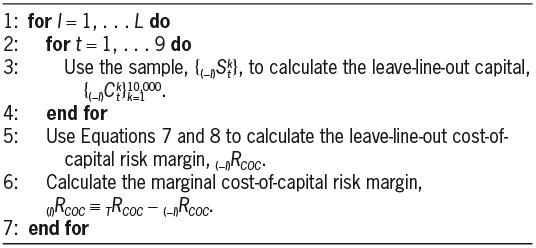
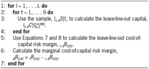
Given the samples, {_lS_t^k}, for each line l of L lines of business one begins to calculate marginal cost of capital for line l, _(l)R_COC, by first executing Algorithm 4 below. Then for each line l execute Algorithm 5.

Algorithm 4.Calculate leave-line-out samples

Algorithm 5.Calculate marginal cost of capital

The fourth column of Table 4.1 gives the marginal cost of capital, _(l)R_COC, by insurer for each line of insurance. Note that the sum of the marginal cost of capitals by line is less than the combined cost of capital in the “Total” column. We then allocate the cost of capital by line of insurance in proportion to the marginal capital by

$$\mathstrut_{(l)} {R}_{A C O C} \equiv \mathstrut_{(l)} {R}_{C O C} \cdot \frac{\mathstrut_{T} {R}_{C O C}}{\mathstrut_{(1)} {R}_{C O C}+\ldots+_{(L)} {R}_{C O C}} \tag{11}$$

Note that there are many instances where the diversification credit is in excess of 80%. This occurs when a “small” line of insurance is part of the portfolio of a “large” insurer. Regardless of what one thinks of allocating the cost of capital, one cannot deny that a small line of insurance adds little to the risk of a large insurer. The insurer size effect illustrated in Figure 3.4 can be significantly reduced by taking diversification into account.

5. One-year time horizon

In the risk margin calculations above, we assumed an “ultimate” time horizon to establish the required capital. Some regulatory jurisdictions, such as Solvency II, specify that the insurer should assume a one-year time horizon. This section extends the methodology of the previous sections to cover the one-year time horizon.

A high-level description of the methodology is to use a Bayesian MCMC model to obtain 10,000 equally likely scenarios that represent the future evolution of the line of business that produced the loss triangle. Then, as new losses come in, one uses Bayes’ theorem to update the probability of each scenario. From those updated probabilities, one can then calculate the statistics that are needed to calculate the risk margin.

Under a one-year time horizon capital requirement, the capital is determined by the estimate of the ultimate losses after one more calendar year of loss experience. A key step in this methodology is to determine the ultimate loss estimate associated with each scenario. For the ultimate time horizon, it is simply U_j. However, as Figure 2.1 illustrates, with only one year of losses from the jth scenario, there may be several scenarios with a significant positive probability.

To get a good approximation, O_t,j, of the expected ultimate loss for the jth scenario, one can simulate future loss experience from the parameter set of that scenario and calculate the ultimate loss estimate, M times. Then set O_t,j equal to the average of those estimates. Algorithm 6 shows the details.

Algorithm 6.Calculate scenario estimates by calendar year

Both the accuracy of the estimate of O_t,j and the computer run time increase with M. After experimenting with different values of M, we found that M = 12 obtained results that were sufficiently accurate given the intrinsic variation of the underlying MCMC simulation.

Algorithm 7 is used to calculate the risk margin for the one-year time horizon. In this algorithm, one simply substitutes O_t+1,j for U_j in the fifth step of Algorithm 1. Given the output of Algorithm 7, one then calculates risk margins using Equations 7 and 8.

Algorithm 7.Calculate capital scenarios for a one-year time horizon

Figures 5.1, 5.2, and 5.3 show the one-year time horizon capital paths, release paths, and risk margins of Insurer #353 for commercial auto that correspond to Figures 2.2, 3.1, and 3.2, respectively, for the ultimate time horizon.

Figure 5.1.Required capital by calendar year

Figure 5.2.Paths of released capital

Figure 5.3.Risk margin

6. Concluding remarks

There has been no universal agreement on the assumptions underlying a cost-of-capital risk margin formula. Beyond the underlying Bayesian MCMC stochastic loss reserve model, this paper makes the following key assumptions:

1. The required assets for an insurer are determined by the TVaR@α measure of risk.

2. The required capital calculation assumes an “ultimate” time horizon.

3. The outcome distributions for the different lines of business are independent.

In numerous advisory committee meetings held at International Actuarial Association events, the author has heard the following argument supporting the one-year time horizon: Insolvency is usually not an instantaneous event. If the insurer finds itself under stress within a year, it will have time to make the necessary adjustments.

At the same meetings the following heuristic definition of a risk margin was also heard: The risk margin is to provide sufficient funds to transfer the insurer’s liability to another insurer. “Sufficient funds” should include the cost of capital.

The following considerations govern our approach to risk margins:

1. The term of such a portfolio risk transfer contract is unlikely to be for a single year, with the risk reverting back to the original insurer at the end of the year. This being the case, we used an ultimate time horizon to determine the capital requirements.

2. For a multiline insurer, the risk being transferred is unlikely to consist of a single line of insurance.

3. Dependency between lines is model dependent. In Meyers (2018) the author demonstrated that the independence assumption is warranted for the CSR model used in this paper.

4. The theoretical advantages of the TVaR@α over the VaR@α have been well documented by Artzner et al. (1999). Whatever computational difficulty there may have been with the TVaR is not an issue with the methodology used in this paper.

Recognizing that reasonable people may differ in their assumptions, this paper points the way to use alternative assumptions. The methodology described in this paper can be readily adopted for any Bayesian MCMC model.