Estimating an Implied Paid Tail Factor: An Application of Shepard’s Method

1. Introduction

Traditional chain-ladder methods are typically based on paid losses or incurred losses, i.e., the sum of paid losses and case reserves. When based on paid losses, an incurred loss tail factor may be used. To do this, the paid loss projection must be converted to an incurred value prior to attaching the tail factor.^[1] In other words, the paid tail factor must be implied using the incurred tail factor and a payout pattern assumption. One simple method to calculate the paid-to-incurred conversion factor is with an average of historical paid-to-incurred (P/I) ratios—the conversion ratio. “Historical” is defined as a year that has reached a development period at or later than the point of conversion.

The application of Shepard’s method^[2] in determining the P/I conversion factor is a distance-weighting of historical P/I ratios, where the distance is based on how closely each historical payout pattern resembles that of a more recent/less mature year.

2. Estimating conversion factors

2.1. The issue of using averages of historical P/I ratios to estimate conversion factors

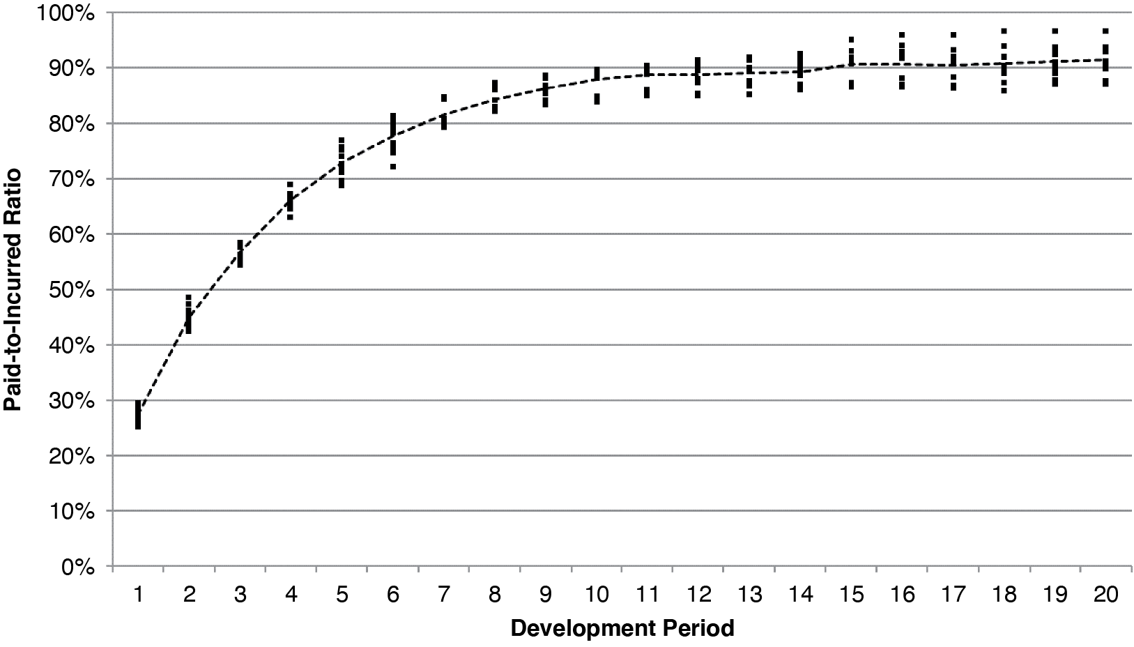
Let us consider a workers compensation portfolio. For this portfolio, the development triangle is used explicitly for the first 20 years, and then a tail factor is attached to arrive at an ultimate loss amount. The paid loss estimate at the end of the 20th year is converted using historical paid-to-incurred ratios prior to attaching the tail factor. The loss payout rate for any individual year may differ from the overall average rate of payout. In Figure 1, 10 P/I ratios are shown at each of the first 20 annual development periods.

Figure 1.A P/I ratio pattern

Conversion ratios applied to the immature years are based on historical P/I ratios at the 20th development period. In response to the range of P/I ratios observed in Figure 1, common practice is to use an average to provide more temperate results. In Table 1, several alternatives are shown.

The use of each alternative averaging method implies an assumption about how losses on an immature year will ultimately be paid. As the number of years included in the average increases (decreases), the less (more) volatile the calculated conversion factor may become. With these averages, two potential issues arise: the calculated conversion may not reflect individual payout patterns of the more immature years, and if new years with largely different payout patterns enter the conversion calculation, the predicted ultimate loss values may abruptly change.

2.2. Applying Shepard’s method to historical P/I ratios

Common averaging techniques of historical P/I ratios rely on a weak assumption that all immature years will pay out similarly to the average payout pattern of the historical years. The distance-weighting of the historical years’ information underlying Shepard’s method may produce conversion factors that better predict the future payout patterns of currently immature years.

To produce a conversion factor for an immature year, we weigh P/I ratios from historical years using their similarity to the immature year. The development periods used to measure similarity will be the most recently available for the immature year. The historical years included in the distance-weighting should provide a sufficient range of potential payout patterns and avoid historical years that may be less relevant to current patterns. Factors that should be considered include, but are not limited to, changes in claim handling, legal reforms that may have affected claim payment patterns, or large shifts in the risk profile of a portfolio.

In Table 2, P/I ratios by development quarter for one immature and 10 historical policy years are compared. The four quarters displayed are the most recently available for the immature year.

Compared with the latest historical years (1992–1996), the relatively lower P/I ratios for the immature year suggest that 2010 may have a relatively slower rate of loss payout. This indicates that using a short-term P/I ratio average for the immature year may be sub-optimal.

To quantify these intuitive conclusions, we must establish a “distance” to use to compare the quarterly P/I ratios for each historical year to those observed for the immature year. Historical years whose P/I ratios are closest to those observed in the immature year should be most heavily weighted in the calculation of the average P/I ratio.

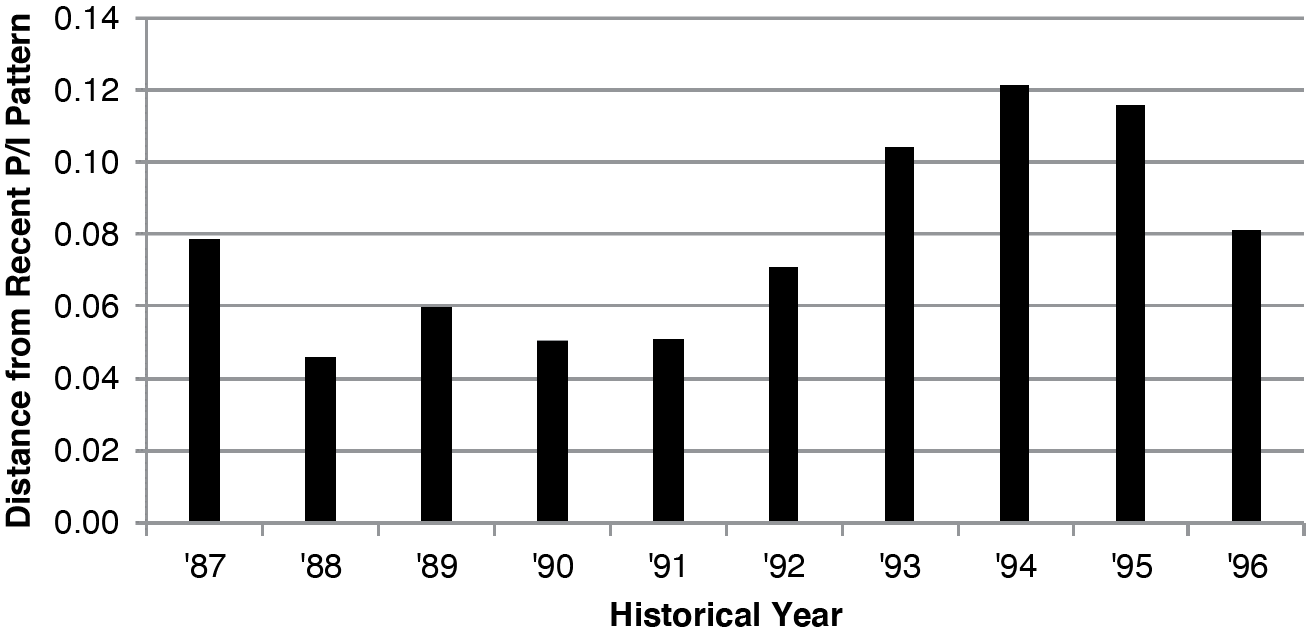
In Figure 2, the distances (see formula in section 2) between the immature year and each historical year are displayed. The historical years with P/I ratios that most closely resemble those of the immature year are those with the smallest distances (Years 1988, 1990, and 1991).

Figure 2.Distance between immature and historical year P/I ratios

Note that the four quarters included in the above calculations contain claim reserve reviews throughout the year. The comparison can be done with more quarters (say 8 or 12) but would lose responsiveness to a changing pattern. On the other hand, using more quarters may increase the stability of the comparison between valuations.

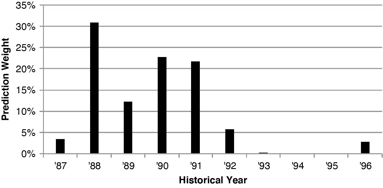
With the distances above, Shepard’s method^[3],^[4] can be used to assign weights to each of the historical years based on the inverse of their relative distance to the largest distance calculated. The largest distance in Figure 2 is observed in 1994, so it will receive zero weight. Weights for the other historical years are determined using the respective relative distances to the immature year (see Section 2 for additional detail).

Figure 3 presents the weights derived from the distances in Figure 2. The historical years with the smallest distances (Years 1988, 1990, and 1991) receive the most weight.

Figure 3.Inverse-distance weights for historical P/I ratios

Using the weights in Figure 3, we calculate a weighted average of the P/I ratios at the conversion period. This is the estimated P/I ratio for the immature year. The inverse of that ratio will be the selected conversion factor.

This method explicitly reflects the expected payout pattern of the immature year, while addressing a primary concern with using traditional P/I ratio averaging techniques when determining the paid-to-incurred conversion factor. Also, based on its construction, the Shepard method may produce results that are less volatile when a year with a largely different payout pattern enters the historical development periods.

2.3. Limits of applying Shepard’s method

This section explores two issues that may arise when using Shepard’s method to estimate conversion factors. First, the immature year’s payout pattern may differ from all the historical years. Second, one or more of the historical payout patterns could be unstable and unfit for prediction.

2.3.1. Unique P/I ratio pattern

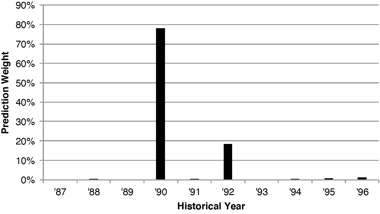
Applying Shepard’s method in this context assumes that the future payout pattern of an immature year will be within the range of those observed in the historical years. When the payout pattern of an immature year is outside the historical range, inverse-distance weighting will heavily weigh one end of the range. This result may not provide a reasonable P/I ratio estimate for the immature year. Table 3 presents an example of this scenario.

In this case, the immature year has comparatively lower P/I ratios than each of the historical years. The weights will be allocated heavily to the years with the lowest P/I ratios. In this scenario, any average P/I ratio using the historical years will be closer to 1.0000 than it likely should be. The Shepard method conversion factor may still understate true ultimate losses, albeit less so than common averaging techniques. The exact weighting of the historical years in Table 3 is shown in Figure 4.

Figure 4.Inverse-distance weights for Table 3

2.3.2. Unstable historical P/I ratio patterns

A historical year may have major, abrupt shifts in its P/I ratio over time. This can happen for several reasons, including large claim emergence, low volume sensitive to small claim fluctuations, reopened claims, and large settlements. Providing significant weight to unstable historical P/I ratios may provide non-intuitive results and/or cause large fluctuations in P/I ratio estimates between valuations.

Applying Shepard’s method will control for this if the development quarters used in the distance calculation are those with large shifts in the payout pattern. The squared distance between P/I ratios for the immature year and those in the historical year will be large—resulting in relatively less weight assigned to that historical year’s information. If, instead, the historical year has large shifts after the quarters used in the distance calculation, it may produce an unreasonable P/I ratio estimate. For example, an immature year developed to Quarter 20 will weigh historical years based on Quarters 20 and prior. If a historical year closes a large claim in Quarter 30, Shepard’s method could incorrectly allocate weight based on the slower payout periods.

The risk of volatile payout patterns in conversion factors is not a new problem. The simpler/traditional averaging techniques will include unstable or otherwise unreasonable P/I ratios if they are the earliest available. In the next section, the NCCI approach to identify abrupt changes in historical P/I ratios will be discussed.

2.4. NCCI’s approach to address the limits of applying Shepard’s method

The following sections will present NCCI’s current approach to address the previously mentioned limitations of applying Shepard’s method. NCCI’s approach was guided by metrics measuring the predictive accuracy and stability of ultimate loss projections based on NCCI’s workers compensation loss reserving portfolios.

2.4.1. Smoothing conversion factor prediction for unique P/I ratio pattern

As seen in section 1.3.1, when an immature year’s payout pattern is unlike those in historical years, Shepard’s method will provide an estimate at one end of the historical P/I ratio range. This over- or under-estimation will continue for each new evaluation period until the point of conversion. If there is a large difference between the estimated value one evaluation period prior to conversion and the actual value at conversion, the ultimate loss projection could change significantly.

To limit the ultimate loss volatility entering the tail development periods, the latest quarterly P/I ratio for the immature year can be weighed with the Shepard’s method estimate. Over the last four quarters prior to tail attachment (Quarters 76–79), the immature year’s latest actual P/I ratio will receive an increasing weight.

The workers compensation portfolio presented in Table 4 (Portfolio 2) demonstrates this conversion factor smoothing.

In this example, the immature year is fully paid out, while all historical years remain active. Any average P/I ratio using these historical years, including one derived with the method described in this paper, will be less than one and would likely overstate the conversion factor and ultimate loss projection. At Quarter 80 and subsequent, the ultimate loss projection will incorporate the actual P/I ratio. This would result in a decrease in ultimate loss in the first tail development period because the applied P/I would be increased.

To minimize any large change in ultimate loss projection, NCCI has implemented a smoothing procedure beginning four evaluations prior to the point of conversion, quarter 80. A demonstration of this can be seen in Table 5.

The final conversion—which includes weighting the Shepard method result with the latest actual P/I ratio—spreads the total impact of the incurred value change across each valuation quarter. The percentage sliding scale is a judgmental selection. Four quarters are smoothed because the P/I ratio is not expected to change much prior to Quarter 80. The earlier the smoothing is applied, the more likely the final estimated conversion factor is overstated. Using the Shepard conversion alone would result in a 2% decrease in ultimate loss at Quarter 80, caused entirely by the conversion factor.

2.4.2. Removing unstable historical P/I ratio patterns

In section 1.3.2, we discussed the impact that unstable historical P/I ratio patterns can have on conversion factor estimation. A stable payout pattern is one that steadily progresses the P/I ratio toward one over time, with limited large changes or reversals. NCCI’s approach to measure payout pattern stability is to fit a curve to the historical P/I ratios and to compare the sum of squared errors to those of the surrounding years.

Figure 5 shows the P/I ratios for a historical year (1988) that contains a noticeable shift at Quarter 74. A logarithmic curve was fit to these ratios to recognize that P/I ratios generally increase to unity at a decreasing rate. The fit uses the latest four development years (16 quarters) to mitigate against large changes commonly observed in early quarters and for easier curve-fitting.

Figure 5.Logarithmic fit to P/I ratio pattern

Table 6 displays the results of fitting curves to the P/I ratios for 10 historical years. If one historical year has a relatively large percentage of the total sum of squared errors observed across the entire 10-year historical period, it may suggest that that year is notably less stable than the others; in this case, NCCI reduces the weight factor calculated using Shepard’s method to zero. This is accomplished by incorporating a penalty factor that is either one (stable year) or zero (unstable year). After a review of accuracy and stability metrics using several percentage thresholds, NCCI chose a threshold of 40%. This resulted in predictions that were largely unbiased, more accurate, and provided stability of ultimate loss projections between valuations.

Historical year 1988 is shown in Figure 5. While this was the least stable of the historical years, it did not comprise more than 40% of the total error and, therefore, was not excluded from the distance-weighting method.

3. Theory and formulas

In this section, we will outline the general formulas for applying Shepard’s method to estimate conversion factors.

Shepard’s method was initially created to interpolate points in irregularly spaced data to create smooth surface models.^[5] This was done with a two-dimensional space and could be generalized for a three-dimensional space. In our case, we will generalize the method to any number of dimensions, which are represented by periods of development time. The focal point of this application will be the inverse-distance weighting formula that determines which surrounding points are most similar to the one being estimated. The surrounding points, in this context, will be the P/I ratios for years that have reached the point of conversion. The estimated point will be the (unknown) P/I ratio at conversion for the immature year.

This method is simple to implement and efficient to calculate.

The conversion ratio is estimated at a selected tail attachment point. Ultimate losses for an immature year are estimated by developing observed paid losses with the product of paid link ratios prior to the tail attachment point, the conversion factor, and an incurred loss tail factor. To begin, we define:

1. \(P_{s,i}\)    Paid loss value at year s and development time i

2. \(f_{i,A}\)    Paid cumulative development factor for development from time i to tail factor attachment point A

3. \(I_{s,i}\)    Incurred loss value at year s and development time i

4. \(Q_{s, i}=\frac{P_{s, i}}{I_{s, i}}\)    Observed P/I ratio at year s and development time i

5. \(\hat{Q}_{s,A}\)    Estimated conversion ratio at year s and the tail factor attachment point A

6. \(T_{s,A}\)    Incurred tail factor for loss valued at year s and tail factor attachment point A

7. \(R_{s, A}=\frac{T_{s, A}}{\hat{Q}_{s, A}}\)    Implied paid tail factor for year s at development time A

An ultimate loss projection is defined:

\[ U L_{s}=P_{s, i} \cdot f_{i, A} \cdot R_{s, A} . \]

The major assumption for actuarial use is that the historical payout patterns are relevant to the patterns of the immature years. It is up to the discretion of the actuary to judge the reasonableness of this assumption. Dramatic changes in claim payout practices may result in distortions. This is similarly true for chain-ladder methods.

Now, we can present the formulas for applying Shepard’s method to P/I ratio prediction. The first step in applying Shepard’s method is to calculate the distance between P/I ratios for the more immature years and those in the historical years for all \(s\) and \(t\):

\[ h_{s, t}=\sqrt{\sum_{x=\max (i \mid t)-(n-1)}^{\max (i l t)}\left(Q_{s, x}-Q_{t, x}\right)^{2}} \]

where \(h_{s,t}\) represents a distance calculated using \(n\) development time periods.^[6] This is calculated for each of the N historical years, \(s\), and a fixed immature year \(t\).

After the distances have been calculated, weight factors are derived for all \(s\):

\[ W_{s, t}=\left[\frac{R-h_{s, t}}{R \cdot h_{s, t}}\right]^{2} \]

where \(R=\max \left(h_{1, t}, \ldots, h_{N, s}\right)\).

The incorporation of penalty factors, \(P_s\), as discussed in section 1.4.2, can be used to produce adjusted weights that are rescaled to sum to unity:

\[ w_{s, t}=\frac{W_{s, t} x P_{s}}{\sum_{s=1}^{N} W_{s, t} x P_{s}} \]

The final estimated P/I ratio is then calculated as

\[ \hat{Q}_{t, A}=\sum_{s=1}^{N} w_{s, t} \cdot Q_{s, A} . \]

As noted in section 1.4.1, the final conversion ratio may be adjusted to limit the influence of historical ratios when immature years’ payout patterns appear largely different than the range observed in the historical years.

This application of Shepard’s method provides a specific \(\hat{Q}\) value for each of the years at development periods prior to the tail attachment point. The favorable characteristics of Shepard’s inverse-distance weighting to estimate P/I ratios include:

1. The weighting of P/I ratios will be limited to those in the portfolio’s history.

2. Distance formulas provide an intuitive recognition of historical payout patterns that resemble those observed in the immature year.

3. Distance formulas are efficient to calculate and easy to implement.

4. Inverse-distance interpolation can be applied to any number of dimensions, i.e., development periods.

5. Distance formulas that include multiple development periods capture the direction of the payout pattern, or whether the P/I ratio is currently moving closer to or farther from unity.

6. Euclidean distance^[7] provides greater penalties to volatile historical patterns than Manhattan distance,^[8] though any distance function can be used.

7. The number of development periods used in the distance formula should be low, avoiding issues with Euclidean distances in high-dimensional analysis.^[9]

8. Shepard’s weighting formula can be implemented across multiple portfolios without further assumptions.

9. Shepard’s method is distribution-free.

4. Complete example and results

In this section, we will provide a full example estimating conversion factors for the initial example portfolio above. For the sake of brevity, the triangle of P/I ratios is suppressed. Table 7 shows the distances between the P/I ratios for each immature year and each of 10 historical years. The distances rely on the most recent four P/I ratios. An example in policy year 2005 is calculated in a footnote.

Next, we will show the R values, which are the maximal h values for each row above. With these, we can calculate the weighting factors.

At this point, the actuary may apply a penalty factor for unstable historical years that are unfit for prediction. For this data, no outlying historical years exceeded the 40% error tolerance described in section 1.4.2, and therefore no penalty factors were used. In Table 9, we show the inverse-distance weights calculated using the weighting factors in Table 8. Note that all rows sum to 100% but may display otherwise due to rounding.

These weights are then applied to the historical year P/I ratios at Quarter 80 shown in Table 10, providing an estimated P/I ratio for each immature year. With the estimated Quarter 80 P/I ratios, we can calculate the final conversion factors. The payout patterns near the conversion development period were within historical ranges, so smoothing was unnecessary.

The boundaries of potential conversion factors (see Table 1) suggest a 3%–15% increase to the paid projection at Quarter 80. In Table 11, we can see that applying Shepard’s method to weigh the historical years’ P/I ratios allows the full range of potential factors to be applied to the differing payout patterns. In contrast, using various averages of historical P/I ratios (see Table 1) would produce results similar to Shepard’s method in only a few years, potentially overstating or understating losses in most years.

To expand on these results, we can look across multiple portfolios. A retrospective test was performed on a mix of small, medium, and large workers compensation portfolios. P/I ratios were estimated using various averaging methods and Shepard’s method for all available years. In Figure 6, we summarize the distributions of squared error percentage values in these estimates across methods. In the error formula on the y-axis, “A” represents the actual P/I ratio at Quarter 80 and “E” represents the expected P/I ratio in prior periods based on the method on the x-axis. The box plots condensed closest to zero suggest the greatest predictive accuracy.

Figure 6.Box plots of squared error percentage by P/I prediction method

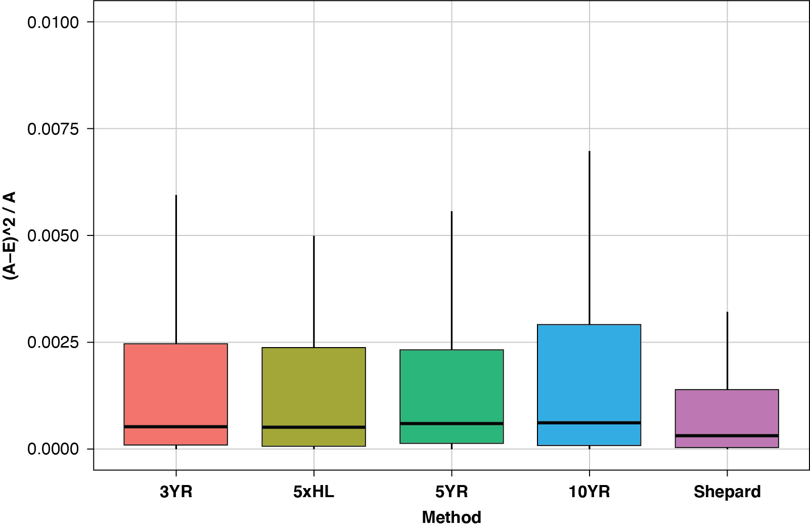
The results of the Shepard method are superior to every averaging method presented, with a reduced median and maximum error.

5. Conclusion

When using paid loss chain-ladder methods to estimate ultimate losses, an incurred loss tail factor can be used with a paid-to-incurred conversion factor to convert developed paid losses to an incurred basis. This implies a paid tail factor from a combination of the incurred factor and the year’s loss payout pattern. We showed that relying on common averaging techniques of the most recent historical years’ P/I ratios may not appropriately reflect the payout pattern of the relatively immature years. Also, large unwarranted changes in P/I estimates may arise when a new year enters the historical averages.

By applying Shepard’s method, we can develop weighted averages of historical P/I ratios that adjust for the payout pattern of the immature year. This method also readily adjusts at each reserve valuation, so large changes in the P/I ratio projections are limited to those justified by changes in the payout pattern. Overall, this method has been shown to reduce error in predicting P/I ratios compared with commonly used averages. These results suggest that Shepard’s method more reliably incorporates information from case reserves in ultimate paid loss indications.

Acknowledgments

I would like to express my gratitude to several people who made my research successful:

My manager, Ia Hauck, and the NCCI Actuarial & Economic Services Division’s leadership for supporting my research into this topic, as well as helping me present it at multiple actuarial forums.

Damon Raben, for his extensive review and suggestions throughout the research, writing, and presentation processes. He consistently challenged and improved my work.

Jay Rosen, Barry Lipton, Kirt Dooley, Sean Cooper, and Erik Miller for their assistance in the final stages of editing and review of the paper.

All the members of the Actuarial Reserving team, who helped to not only review but also implement this new method at NCCI.