A Bayesian Approach to Excess of Loss Pure Premium Rating

1. Introduction

When pricing excess of loss (XOL) programs, many reinsurance and large account pricing actuaries may rely on assumptions that are difficult to support. This is particularly true when the actuary is uncertain of the underlying exposure or of which exposure curve(s) to use. An additional complication arises when the reinsurer does not receive all individual claims in the reinsurance submission, because claims are typically reported only above some truncation point. Finally, maximum likelihood estimation (MLE) and, by extension, Bayesian analysis is generally not amenable to modeling long-tailed lines of business in which claims tend to develop upward or downward over time. This paper attempts to solve all of these problems within a single coherent framework.

Meyers (2005) provides a Bayesian methodology for estimating loss costs associated with high layers. An introduction to the methodology can be found as a solution to the COTOR Challenge. It’s been many years in the making, but Meyers’ solution to the COTOR Challenge was a primary motivation for much of the work I have done here. Following his solution to the COTOR Challenge, Meyers offers solutions to address what he feels are two serious shortcomings of the methodology: (1) the way in which prior severity models were developed and (2) the effect of settlement time on ultimate value. These are major issues for which this paper offers two more solutions. Finally, the framework presented here includes a Bayesian estimate (the mean of the posterior loss ratio distribution) for the ground-up loss ratio. Actuarial literature is relatively absent any discussion of Bayesian loss ratios for XOL rating.

Gelman (2006) distinguishes three categories of priors: (1) prior distributions giving numerical information that is crucial to estimation of the model—such a prior would be a traditional informative prior, which might come from a literature review or explicitly from an earlier data analysis; (2) prior distributions that are not supplying any controversial information but are strong enough to pull the data away from inappropriate inferences that are consistent with the likelihood—this type of prior might be called a weakly informative prior; and (3) prior distributions that are uniform, or nearly so, and basically allow the information from the likelihood to be interpreted probabilistically—such priors are noninformative priors or maybe, in some cases, weakly informative. The approach taken here uses a weakly informative prior for the prior severity distributions. The prior loss ratio distribution is implied by the prior severity distributions (as described in section 5).

When significant claim volume is available, accurate severity distributions can be estimated by using empirical methods, nonparametric statistics, or maximum likelihood methods (Klugman, Panjer, and Willmot 2009). When little or no data is available, actuaries may rely on an exposure curve. There are numerous approaches for deciding upon an exposure curve. For example, one can use an external curve acquired from a statistical agency or an internal curve developed from a similar business line. In the limiting case, where there is no data, the Bayesian approach defaults to the average of the prior distributions. In such cases, with little or no data, it becomes useful to calibrate prior severity distributions to agree with the exposure curve selected for the underlying insured. In such a case, we prefer an informative prior. As the volume of claim data grows, it becomes less critical for the average of the priors to agree with the exposure curve selected for the underlying insured. This paper does not assume that an exposure curve underlying the insured risk is available. A Bayesian approach is most useful when we are between the two extremes of no data and a significant volume of data. The posterior severity distribution can be viewed as a nonlinear weighing of data and prior curves.

Prior to the application of the model, it will be assumed that the premium is on level and losses have been properly adjusted for trends and changes in attachment points and limits. Improper adjustments may lead to estimates with greater error.

Section 2 outlines how the severity distribution and the likelihood function can be adjusted for age of claim. This is accomplished through estimating claim count emergence patterns from various sizes of loss triangles and applying these patterns directly to the likelihood function. Section 3 examines 24 severity distributions used as priors for Bayesian analysis purposes. Using “only” 24 curves is a relatively simple implementation of the approach. The curves are not meant to be prescriptive but are selected for illustrative purposes.

Section 4 describes the assumptions and sample data (one simulation) underlying the model. Section 5 describes the process of estimating an underlying loss ratio for each curve using MLE. Section 6 describes the calculation of the posterior weight for each curve. Section 7 describes a Bayesian approach for estimating the ground-up loss ratio weighting over all MLE estimates, also called the mean of the posterior loss ratio distribution. Section 8 compares Bayesian claim count estimates with experience and MLE estimates for 200 sets of data (simulations). Section 9 summarizes and concludes.

2. Adjusting the likelihood function

The likelihood function is the probability of observing the specified data, given a hypothetical value of the parameter. In the example presented here, the data is the number of reported claims in each layer and the hypothetical parameter is a hypothetical severity distribution. The MLE estimate is the distribution yielding the highest probability of obtaining the observed reported claim counts, weighted over all layers. However, in the case of liability business, data is immature. Ultimate claim counts by layer will generally not be the same as reported claim counts by layer. In general, curves fitted to reported and to ultimate claim counts utilizing MLE will not produce the same parameter estimates.

Reported claims may be available, but can we get the severity distribution for ultimate claims? The form of the likelihood function used in this paper is based on grouped data. Let a range of possible values be partitioned as $c_0<c_1<\ldots c_k$, where $c_0$ is the smallest possible value in the model (i.e., the truncation point) and $c_k$ is the largest possible value (i.e., the maximum policy limit). Let $\left[F\left(c_j ; \theta\right)-F\left(c_{j-1} ; \theta\right)\right]$ represent the proportion of ultimate claims in the band $c_j$ to $c_{j-1}$, given the distribution $F$ and parameter $\theta$. The grouped likelihood function is given by the expression

$$L(\theta)=\prod_{j}\left[F\left(c_{j} ; \theta\right)-F\left(c_{j-1} ; \theta\right)\right]^{n_{j}}, \tag{1}$$

where $n_j$ is the number of claims in the band. Note that the proportion of claims for the reported data will differ from ultimate claim counts by the emergence pattern. In other words, the relative proportion of claims reported in each band is the following:

$$\% \text { Reported }_{j} x\left[F\left(c_{j} ; \theta\right)-F\left(c_{j-1} ; \theta\right)\right]. \tag{2}$$

For reported claims, the proportion of claims in each band is

$$\begin{array}{l} \% \text { Reported }_{j} x\left[F\left(c_{j} ; \theta\right)-F\left(c_{j-1} ; \theta\right)\right] / \\ \qquad \sum_{j} \% \text { Reported }_{j} x\left[F\left(c_{j} ; \theta\right)-F\left(c_{j-1} ; \theta\right)\right]. \end{array} \tag{3}$$

The denominator is simply a normalizing constant so that the probabilities sum to unity.

The adjusted likelihood function for reported claims is

$$\begin{aligned} L(\theta)= & \prod_{j}\left\{\% \operatorname{Reported}_{j} x\left[F\left(c_{j} ; \theta\right)-F\left(c_{j-1} ; \theta\right)\right] /\right. \\ & \left.\sum_{j} \% \text { Reported }_{j} x\left[F\left(c_{j} ; \theta\right)-F\left(c_{j-1} ; \theta\right)\right]\right\}^{n_{j}} . \end{aligned} \tag{4}$$

Exhibit 2.1 illustrates one way we might simulate reported claim counts from a lognormal distribution with an underlying emergence pattern. Only 10 of 30,000 simulations are displayed. Column (2) represents an ultimate claim value. At any point in time, the estimated claim value may be more, or less, than the ultimate value. We are assuming an emergence pattern as shown in column (9). Smaller claims, from $0 to $100K, are assumed to be reported more quickly. We assume that 90% of all claims less than $100K have been reported and that of the largest claims, only 60% have been reported. It is common for reinsurers to examine separately the incurred and paid claim count triangles by size of loss. To convert ultimate counts to reported counts, we first augment the emergence pattern, shown in column (3). A unit-uniform random variable is generated, shown in column (4). If the random variable is less than the emergence pattern [i.e., if column (4) column (3)], the claim is considered reported [column (5) = 1]. If the claim is reported, it is shown in column (6). At this point, roughly 90% of the claims less than $100K show up as reported claims in column (6), while only 60% of the claims from $2M to $4M show up as reported.

Exhibit 2.1.One way to simulate reported claim counts from a lognormal distribution with an underlying emergence pattern

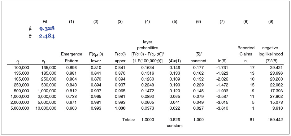
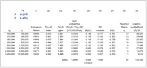
Exhibit 2.2 illustrates the application of equation (4) to the reported claim counts simulated in Exhibit 2.1. In practice, it is typical to minimize the negative log-likelihood function, $-\ln [L(\theta)]=\Sigma_j n_j \ln [(3)]$. Minimizing column (9) produces the parameters shown in the upper left of the exhibit. We can see that the fit is in close agreement with the underlying severity parameters, or “actual.”

Exhibit 2.2.Application of equation (4) to reported claim counts simulated in Exhibit 2.1

So what does this exercise tell us? It tells us that if we have reported claim amounts (counts) and an estimate of the emergence pattern, we can replicate the parameters of the underlying severity distribution, and we are well on our way to implementing a Bayesian approach. Why not just use adjusted MLE rather than a Bayesian approach? Because we usually don’t see 25,655 reported claims [the total of column (8) in Exhibit 2.2]. Fewer claims leads to greater parameter uncertainty underlying the MLE estimates. For smaller portfolios, Bayesian estimates utilizing the mean of the posterior distribution are less impacted by random variation than are MLE estimates. Krishnamurthy (2017) provides an illustration of and explanation for this case. However, the adjusted MLE does seem especially well suited for pricing very large portfolios or creating exposure curves for individual lines of business.

3. Prior distributions

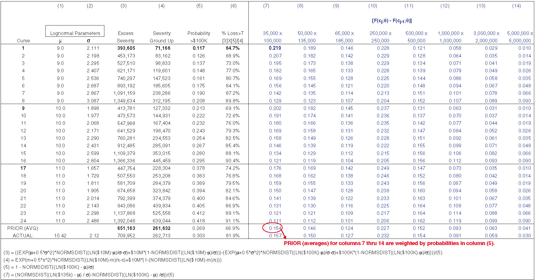
For this paper, we implement just 24 severity distributions as priors. Exhibit 3.1 displays the parameters and some statistics for the 24 curves. The mean of the prior distribution is an equal weighted average of the curves, labeled “PRIOR (AVG)” (the excess severity is also weighted by the probability of a claim’s exceeding the truncation point, $100K). “ACTUAL” denotes the statistics associated with the lognormal curve in section 2. It should be noted that statistics and probabilities for the prior curves are net of any insurer attachment/limit profile. These figures can be calculated easily in most exposure rating models. For the implementation here, I have selected lognormal curves for prior distributions. Although we may be unsure of the underlying stochastic process, I have found that in most cases this choice of prior produces a reasonable estimate of the underlying severity distribution even when the underlying process is not lognormal. However, using priors that better match the distributional form generally produces estimates with lower variance and bias. I suggest that readers identify the most appropriate distribution underlying their data and use priors that match that distribution. This exposition uses expressions and calculations for the lognormal distribution. MLE is one possible approach for identifying the distribution. Given the same number of parameters, one could select the distribution that produces the greatest value of the likelihood function.

Exhibit 3.1.Prior severity distributions

How might prior severity distributions be constructed? Assume we are pricing a $5M excess $5M layer on a per-occurrence basis and receive only claims above some truncation, say $100K.^[1] To calibrate the curves as shown in Exhibit 2.2, and in general, the following procedure can be utilized. Examine the company’s exposure curves. What are the lowest and highest probabilities indicated by the curves for the highest layer, $5M × $5M? The prior severity distributions should span the low and high probabilities indicated by the curves. For the exposure curves available to me, a range from 1% to 9% was sufficient. These figures represent the proportion of claim counts above $5M, given only claims above $100K. Next, I’ve judgmentally selected three scale parameters: 9, 10, and 11. With the given scale parameters, I use Excel’s solver to find the shape parameters to match the target probabilities shown in Exhibit 3.1, column (14). In practice, I suggest using more than three scale parameters and extending the range of probabilities beyond the highest and lowest indicated by the exposure curves. Extending the ranges reduces the bias that may result when rating an account that tests the extremes of the prior severity curves.

4. Assumptions and “data”

The following discussion assumes an identical severity distribution for each risk. This is an appropriate assumption for testing the efficacy of the model. The underlying ground-up loss ratio for each risk will vary. Since each risk is of identical severity, the impact of the loss ratio is felt through the frequency of claims.

In the example that follows, “data” will be the result of one simulation, to which we fit the model. We simulate an emergence pattern, a ground-up loss ratio, and the size of claim(s). The Bayesian approach will simultaneously fit both the severity distribution and the ground-up loss ratio. We examine 10 years of losses with the following additional assumptions: a $6M premium is written each year, and the loss ratio is drawn from a lognormal distribution with mean 100% and coefficient of variation 20.2% (σ = .2).^[2] Size of loss is drawn from a lognormal distribution with parameters as shown in Exhibit 2.1, μ = 10.42 and σ = 2.12. Maximum loss size (the policy limit) is $10M. The expected annual number of ground-up claims over all risks is 22.8 ($6M divided by an expected severity of $262,713). However, for each risk, the expected frequency varies as a function of the underlying loss ratio. We assume that the reinsurer receives only those claims above $100K (due to truncation: T = $100K). Given this lognormal assumption, roughly 6.9 claims per year are in excess of $100K (69 claims over 10 years). Based on simulated emergence patterns, roughly 78% of these claims are reported. The percentage reported declines as the size of loss increases. Frequency is simulated from a negative binomial distribution with a variance-to-mean ratio of 1 + cL, with c = .01^[3] and where L is the expected number of ground-up claims.

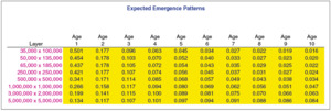
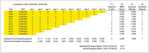
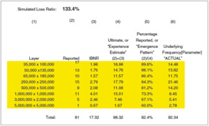
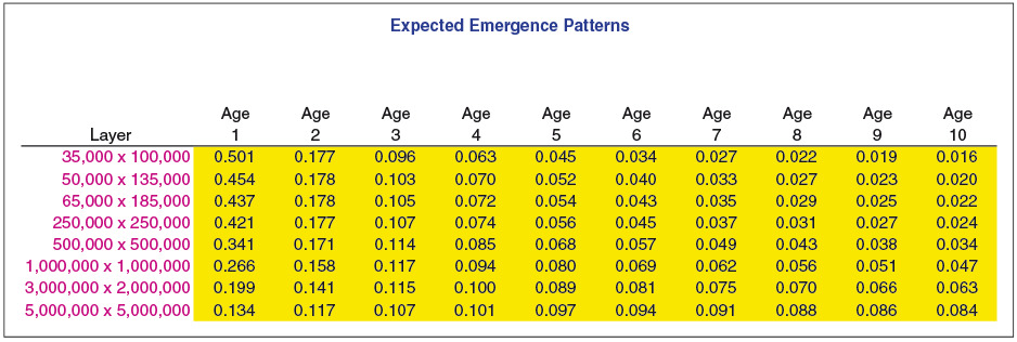
Exhibit 4.1 displays the expected emergence pattern for each of the layers (bands) of loss. The emergence patterns are unknown parameters and are therefore estimated. This paper suggests an approach to estimating these patterns, but that is not a goal of the model. Losses are reported more quickly for lower layers than for higher layers. The variation around the expected pattern for each age is modeled as lognormal with a sigma of 50%. After emergence patterns are simulated for each age, they are scaled so that the patterns add up to unity for each accident period. Exhibit 4.2 displays the reported claims, ultimate claims, estimated emergence pattern, and actual emergence pattern for the $3M × $2M layer. Since each year has identical exposure, the incremental claim count pattern can be calculated simply as the incremental number of claims reported in the lag period (the development period) divided by the years of data for that age. For example, in the triangle shown in Exhibit 4.2, one claim is reported from age 1 to age 2 (over accident periods 2007 through 2015). This results in .111 claims expected to emerge from age 1 to age 2 (1 claim over 9 years). For 10 years of data, 5 claims have been reported to date, 7 ultimate claims have been simulated, and we estimate 2.46 claims incurred but not reported (IBNR). The estimated percentage reported for the $3M × $2M layer is 67.1% (5/[5 + 2.46]). The 67.1% will be the $3M × $2M contribution to adjust the 24 severity distributions to a reported level. Exhibit 4.3 displays the simulated loss ratio, reported claims, IBNR claims, ultimate claims, and estimated emergence pattern (percentage reported) for all the layers. The simulated loss ratio is an unknown parameter, which the Bayesian framework will estimate. The reported claims and the ultimate claims are totals over 10 years. Column (4), “Ultimate,” represents an “experience” or “emergence” estimate. The Bayesian estimate will be compared with this estimate.

Exhibit 4.1.Expected emergence patterns

Exhibit 4.2.Reported claims, ultimate claims, estimated emergence pattern, and actual emergence pattern, $3M × $2M layer

Exhibit 4.3.Simulated loss ratio, reported claims, IBNR claims, ultimate claims, and estimated emergence pattern, all layers

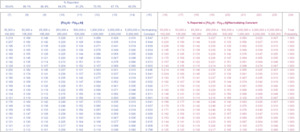
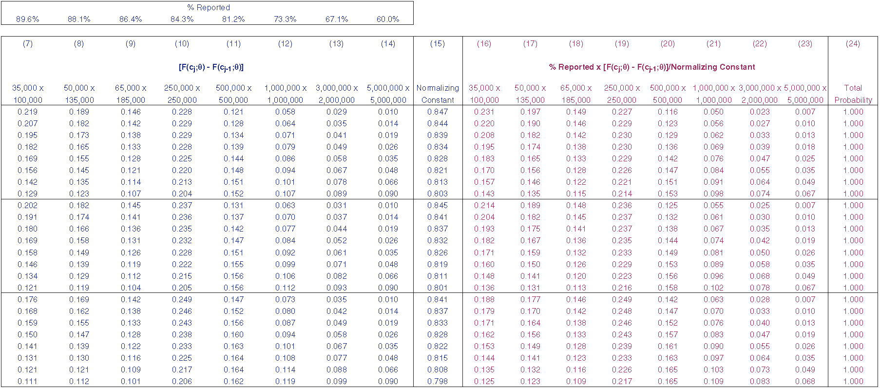
The adjustment of the severity distributions to a reported basis from an ultimate basis is shown in Exhibit 4.4. At the top left of the exhibit is the emergence pattern, or percentage reported, in each layer (see Exhibit 4.1). Examining layer probabilities reveals that adjusting the distributions shifts some probability from the higher-attaching layers to the lower-attaching layers.

Exhibit 4.4.Ultimate and reported probabilities

5. MLE estimate for the ground-up loss ratio

For each curve, we can calculate the probability of a claim’s exceeding the truncation (T = $100K), along with the ground-up and excess claim severities. Given a ground-up loss ratio, it is possible to estimate the ground-up claim count and the number of claims in excess of a given truncation point. Recall that we started our example (or analysis) with an estimate of the total on-level premium for all years. Applying a loss ratio produces total loss, total ground-up claim counts, and the number of claims above the truncation.

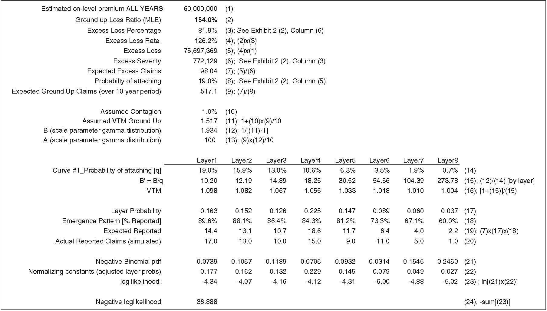
Also for each curve, given a loss ratio, we can estimate the expected number of claims in each layer. Applying the emergence pattern (Exhibit 4.3) to these counts gives us the expected number of reported claims in each layer. We can assume a frequency distribution for each layer and solve for the loss ratio that maximizes the likelihood of observing the reported claim counts in each layer, given the expected number of reported claims in each layer. Under this framework, we can view the loss ratio as a parameter of the frequency distribution. For the ground-up claim counts, we assume a negative binomial distribution with a variance-to-mean (VTM) ratio of 1 + cL, with c = .01 and where L is the number of ground-up claims as a function of the MLE. The model is robust to the choice of c. The maximum likelihood function is the product of eight frequency distributions normalized for probability in each band; the probability in each band can be found in Exhibit 4.3, columns (16) through (23). Normalizing assures us that the total probability summed over the eight frequency distributions is 100%. Normalizing doesn’t affect the MLE for each curve, but it does affect the relative likelihood between curves, which in turn influences the ground-up loss ratio (i.e., the mean of the posterior loss ratio distribution) weighted over all curves (more in section 7).

The VTM ratio generally declines as we move up into successively higher layers. Patrik and Mashitz (1990) describe expressions that modify the ground-up VTM ratio as we move into higher layers. We can view the dispersion in the ground-up claim count as the result of independent Poisson random variables, each with a different underlying mean. We assume the mean is gamma distributed, with parameters A and B calibrated to produce the observed ground-up claim count and VTM ratio. Expressions are as follows:

$$\text{Ground-up claim counts} = A/B$$

$$\text{VTM ratio} = (1+B)/B$$

$$\text{Ground-up parameters are } B = 1/(VTM-1)$$

$$A = (\text{Ground-up counts}) \times (VTM - 1)$$

As we move into higher layers, Patrik and Mashitz proceed to show that the scale parameter B B/(probability of attaching). The expression for the VTM above gets updated as B gets transformed. The probability of attaching is calculated directly from the prior severity distribution.

Exhibit 5.1 takes us through the calculations for curve #1 (see Exhibit 2.2 for parameters). The MLE estimate shown on line (2), 97.8%, minimizes the negative log-likelihood function on line (22). The negative binomial density function on line (19) evaluates the probability of observing the actual number of reported claims, given the number of expected reported claims and the VTM ratio. The expected number of claims is a function of the ground-up loss ratio. An identical calculation is performed for each curve.

Exhibit 5.1.MLE estimate of the ground-up loss ratio for curve #1

6. Posterior weights for the severity distribution

The severity likelihood function depends on two expressions. The first expression is equation (4) above, the adjusted likelihood function. The second expression will be described below.

It is quite common that only claims in excess of some given truncation are submitted to a reinsurer. In many instances, a severity distribution that appears to be a good candidate (fit) from an excess perspective may not be a good candidate from a ground-up perspective. Why does this matter? Because in many instances, curves that seem to fit well just above the truncation point do not adequately capture the tail of the underlying severity distribution. A curve that fits well on an excess basis might imply a loss ratio significantly or implausibly different than expected. Therefore, we examine the MLE for the ground-up loss ratio. If the MLE is significantly different than the expected loss ratio (ELR), the curve is not a good candidate for the underlying severity distribution. The ELR can be the result of a detailed analysis for the individual risk, or it can be the result of an industry study. Given estimates of the ELR, uncertainty surrounding the ELR, and the process risk underlying the frequency and severity assumptions, we can calculate the likelihood of observing the MLE. This is the second expression mentioned above.

For our case study, we assume that ground-up triangles are not available, and we utilize a mean industry loss ratio of 100%, with individual risks varying around this mean loss ratio. We will assume a lognormal distribution with σ = 40%. Our estimate of the dispersion around the ELR is considerably wider than the underlying 20%. Again, we will assume the MLE is lognormally distributed with mean 100% and σ (.4² + process variance)^.5, where the process variance is calculated assuming the underlying ELR of 100%. For the likelihood, we calculate the density of the MLE using the parameters above. For this calculation, we use Excel’s built-in function LOGNORM.DIST. Exhibit 6.1 takes us through the calculation for curve #1. The calculation assumes that the premium charged for excess losses mirrors the ELR. A discussion of each term used to calculate the process variance is beyond the scope of this paper. However, analytical expressions are defined in Exhibit 6.1. We use simulation to validate the process variance.

Exhibit 6.1.Likelihood of the MLE, given the ELR and total variance for curve #1

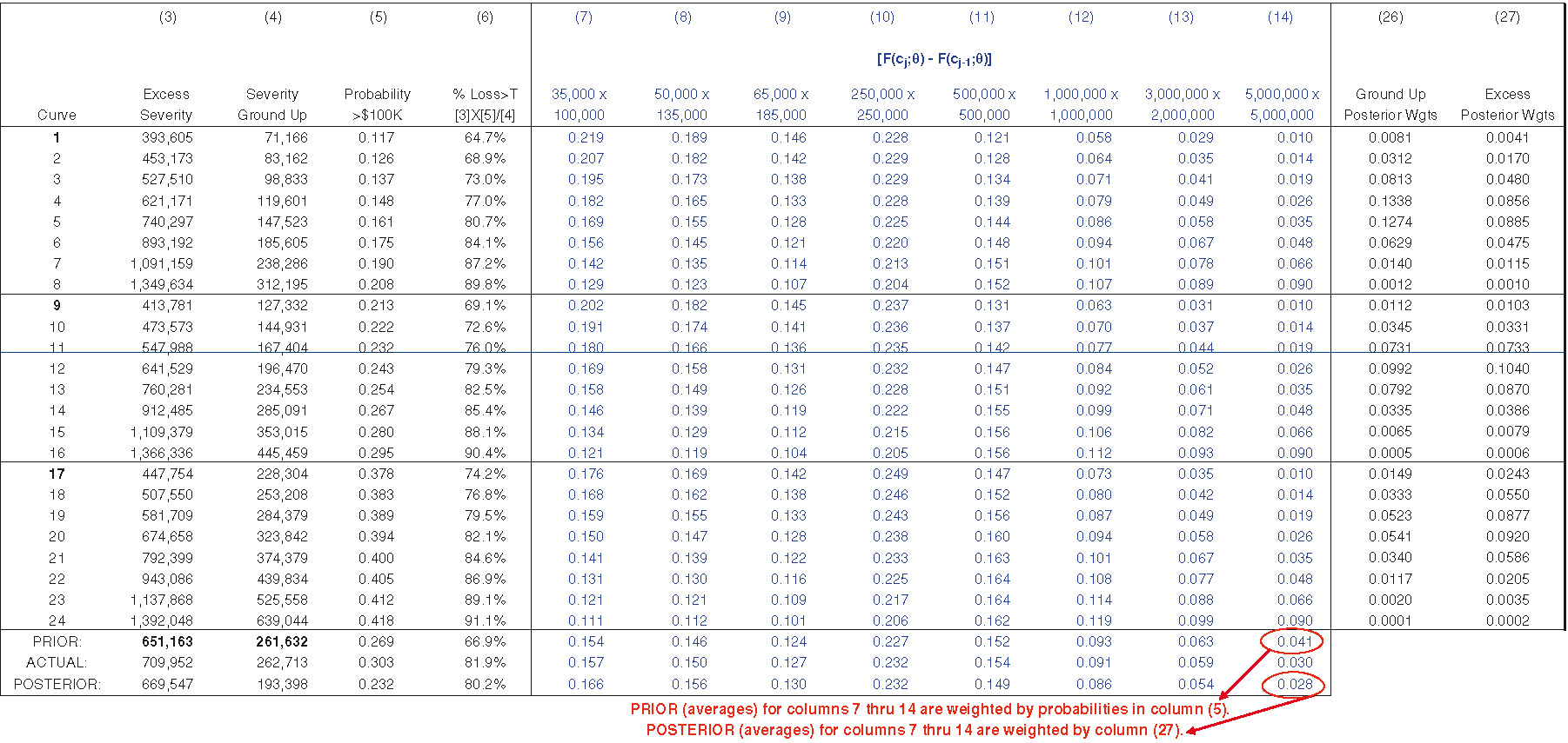
Exhibit 6.2 displays the posterior weight for each severity distribution. Columns (26) and (27) display ground-up weights and excess weights. Equation (5) states the posterior weight as proportional to the product of the probability of the data given the model, also called the likelihood, and the prior probability. Since prior weights are equal, posterior weights are proportional to the likelihood function.

$$\begin{array}{c} \text {Posterior}\{\text{model} \mid \text{data}\} \propto \text {Probability}\{\text{data} \mid \text{model}\} \\ \times \text {Prior}\{\text {model}\} \end{array} \tag{5}$$

Exhibit 6.2.Posterior weights for severity distributions

Ground-up weights are necessary to calculate ground-up statistics such as ground-up severity, while excess weights are used to calculate excess statistics. For informational purposes, the MLE for each curve is shown in column (28). One can see that the likelihood of the MLE, and thus the weights, declines as the MLE deviates from the ELR. The likelihood function in column (24) may potentially create numerical underflow problems. One possible way of handling this is by taking logarithms of each term in the likelihood function, adding the absolute value of the smallest log-likelihood value to each log-likelihood value, exponentiating the results, and then normalizing.

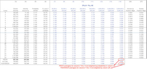
Exhibit 6.3 displays the posterior severity distribution. To create Exhibit 6.3, we append columns (26) and (27) from Exhibit 6.2 to Exhibit 2.2. The last row of columns (7) through (14) of Exhibit 6.3 represents the posterior severity distribution, conditioned on claims greater than the truncation. It is important to note that given the statistics in the last row of columns (3) through (6), and an estimate for the ground-up loss ratio, claim count estimates for the eight bands can be produced. We will refer to these claim count estimates as Bayesian claim count estimates, or Bayesian estimates. It is also instructive to note that curve #12 produces the greatest likelihood (posterior weight) of generating the observed data. Looking back at Exhibit 2.2, we can see that compared with the other curves, the parameters and statistics for curve #12 are relatively close to the underlying, or ACTUAL.

Exhibit 6.3.Posterior severity distribution

7. The ground-up loss ratio (mean of the posterior loss ratio distribution)

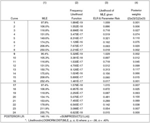
As described in section 5, an MLE estimate for the ground-up loss ratio is derived for each curve. We can view these estimates as a set of priors, all initially receiving equal weight. As with the severity distribution, the likelihood of each MLE estimate depends on two expressions. The first expression can be found on line (21) of Exhibit 5.1. However, instead of transforming the likelihood to a negative log-likelihood, we will rely directly upon the likelihood function. To convert the 43.1159 negative log-likelihood found in Exhibit 5.1, we change sign and exponentiate: e^−43.1159 = 1.884E – 19. The second expression is described below.

The eight frequency distributions, one for each layer, are a function of the MLE. As with a severity distribution, a frequency distribution that may be a good candidate for the excess frequency may not be a good candidate for the underlying ground-up frequency. Again, if the MLE is significantly different than the ELR, the MLE is not a good candidate for the underlying frequency distribution. Whereas process risk should be recognized when identifying which severity curves could potentially produce the observed data, the expected process risk underlying each curve should not be reflected when calculating the likelihood of the MLE given the ELR and the surrounding uncertainty (i.e., the parameter uncertainty). Our second expression reflects only this parameter uncertainty. As described above, we assume an industry loss ratio of 100% with individual risks lognormally distributed and σ = 40%.

Exhibit 7.1 displays the calculation of the ground-up loss ratio, which is a weighted average over all MLEs. In this example, the underlying, or ACTUAL, loss ratio is 133.4%, while the posterior loss ratio is 146.1%.

Exhibit 7.1.Mean of the posterior loss ratio distribution

Exhibit 7.2 ties together the posterior severity distribution in Exhibit 6.3 with the mean of the posterior loss ratio distribution in Exhibit 7.1 to arrive at Bayesian claim count estimates. We can see that the Bayesian count better mirrors ACTUAL (the underlying frequency/parameter) than does the experience estimate. An experience approach is more responsive to the reported claims in the layer and is thus more responsive to random variation. Exhibit 4.3 shows that only 1 claim has been reported at the 5 × 5 layer, while the true underlying frequency is 2.78 claims. Thus, experience rating is too responsive to the reported claim counts. Where reported claims are higher than the underlying expected reported claims, experience rating tends to produce an estimate that is too high. Where reported claims are lower than the underlying expected reported claims, experience rating tends to produce an estimate that is too low. A Bayesian approach takes into account experience in all layers and does not overreact to random variation to the degree that experience rating does.

Exhibit 7.2.Projected claim counts

8. Bayesian estimates versus MLE and experience estimates

Exhibit 8.1 displays an extract of Bayesian, MLE, and experience fits (estimates) for 200 sets of simulated data; 200 is enough simulations to be an effective illustration of expected results. The MLE approach utilizes parameters as estimated by the methods discussed above: specifically, the adjusted likelihood function, as in equation (3), and the MLE estimate for the ground-up loss ratio, as shown in section 5. The calculations for simulation 1 can be found in appendix A. We use estimated emergence patterns for the experience estimates.^[4] For ease of exposition, only the top three layers for each approach are shown. Columns (1) through (3) are Bayesian claim count estimates, columns (4) through (6) are MLE estimates, and columns (6) through (9) are experience estimates. Each set of claim count estimates relies on the same estimated emergence pattern. We also show the underlying, Bayesian, and MLE loss ratios. The underlying loss ratio is the simulated loss ratio, while the Bayesian and MLE loss ratios are estimates. The last column, (13), is the underlying frequency for the $5M × $5M layer for each simulated set of data. This is the parameter we are attempting to estimate.

Exhibit 8.1.Bayesian versus MLE and experience claim count estimates (over 10 years)

The average of the Bayesian loss ratios shown in Exhibit 8.1 is 105.8%, while the underlying parameter for these 200 simulations is 98.6%. Some of this loss ratio bias is due to the choice of prior curves; however, the bias may also “force” expected counts to more closely mirror reported counts. It is difficult to come up with general rules for constructing prior severity distributions. Not only can the choice of curves reduce or increase bias, but it also affects variance. This trade-off should be tested in the development of prior curves. MLE loss ratios exhibit less bias than Bayesian loss ratios, but their mean square error is significantly greater.

The “actual” number of claims for each layer is shown in column (13). “Actual” represents the underlying parameter, not the actual simulated counts. Simulation 1 represents estimates for the sample data. For each simulation, any deviation from “actual” is due to process risk. The goal of any model is to produce estimates that are both unbiased and have minimum variance. Exhibit 8.1 shows that the experience and MLE estimates tend to have slightly lower bias but much higher variance than the Bayesian estimates. It is worth noting that in some instances, actuaries will price higher layers by applying increased limit factors (ILFs) to lower layers, where there is more experience. In this case, Exhibit 8.1 suggests that pricing would be improved by applying the ILF to the Bayesian estimate for the lower layer. However, deciding which ILF to utilize still requires judgment, while a Bayesian framework is objective in nature.

Exhibits 8.2 and 8.3 are pricing exercises of the Bayesian framework contrasted against the experience and MLE approaches. We assume that an insured will select the lowest of the prices offered in the market. For the 200 simulations, we assume 0% expense and profit loads. For calculating pure premium, the experience approach utilizes experience frequency and the actual underlying severity. For the Bayesian approach, severity is a posterior weighted average of the individual severities for each curve. For the MLE approach, severity can be calculated directly. For contrasting the Bayesian and experience approaches, using actual severity for the experience rate is conservative. The simulations have been sorted in descending order of loss ratio and separated into five quintiles, allowing us to do some testing to determine whether the Bayesian model is picking up differences in loss ratio.

Exhibit 8.2.Pricing exercise: Bayesian approach versus experience approach

Exhibit 8.3.Pricing exercise: Bayesian approach versus MLE approach

Based on the 200 simulations found in Exhibits 8.2 and 8.3 (showing only the first 10 simulations), if a competitor were to use rates indicated by the experience and MLE approaches, it would write less business at a significantly higher loss ratio. We can also see that the Bayesian approach does a reasonably good job of reflecting loss ratio differences. Recall that we assume an ELR of 100% with a parameter coefficient of variation of 40%. For risks with the highest loss ratios, the top 20%, the model estimate is 130.2%, while the actual is 128.9%. This should alleviate some concern regarding adverse selection. There are 40 simulations in each quintile. The profit or loss is the sum of all simulations in the quintile. The other statistics are averages for the quintile. We can see that the Bayesian loss ratio tracks the underlying loss ratio reasonably well, and that a Bayesian underwriting profit is produced for each quintile.

Exhibit 8.4 is a head-to-head comparison/competition of all three approaches.

Exhibit 8.4.Pricing exercise: Bayesian approach versus MLE and experience approaches

9. Summary and conclusions

XOL rating generally requires an exposure curve, a loss ratio, and a credibility procedure to weight experience and exposure estimates. In many instances, at least one and sometimes all three of these parameters are judgmentally selected. Just as experience or MLE estimates can overreact/overfit to random variation in the data, so can actuarial judgment. When we see higher-than-expected loss, we tend to pick conservatively. When we see lower-than-expected loss, we are optimistic. The author believes that relying on judgment may produce results no more accurate, and possibly even less so, than the experience and MLE approaches presented in this paper. Another drawback of approaches that utilize too much judgment is that they are difficult to monitor or recalibrate.

This paper provides a Bayesian framework for XOL rating. There are many possible variations on the approach provided here, each providing possible advantages and/or disadvantages. These variations include the family of prior distributions, how the curves are calibrated, the number of layers utilized, and the introduction of credibility into the procedure. The approach taken here can be viewed as a starting point, or “Barnett approach.”

The author believes that a single set of prior severity distributions allows for the development of a model that could be monitored for performance and recalibrated over time (a technical price can be constructed and compared with actual results to potentially recalibrate the model). Based on the volume of losses simulated in the exhibits above, in my opinion, it is preferable to develop a single set of prior severity distributions that fit well to a wide range of potential losses (severity distributions) and produce results similar to those above.^[5]

Readers may be tempted to develop separate sets of curves for different risks, or lines of business, so I offer a word of caution: try to develop an objective set of standards that clearly define under what circumstances each risk will be assigned to a set of curves. Otherwise, a technical price is difficult to monitor and recalibration becomes problematic. Another issue with separate sets of curves is bias. Presumably, separate sets are developed to capture differences in severity potential. A risk that is not properly assigned could potentially lead to greater bias. However, if risks are properly assigned, we generally find an estimate with lower mean square error.

It should be noted that biased low estimates can still be profitable relative to traditional pricing techniques, suggesting that narrow priors with some bias are acceptable. However, this is a function of the relative variance. If a competitor can produce unbiased estimates with comparable variance, it is likely that the biased low portfolio will be unprofitable.

Even if the risk exposure is well known and an exposure curve is available, a Bayesian approach may be preferable if the exposure curve is not properly constructed. Improperly constructed curves may lead to bias in all business priced. A Bayesian approach could be preferable even when a properly constructed exposure curve is available. Recall that an exposure curve may be accurate for all risks in aggregate, but it is unlikely that all risks share the same underlying severity propensity.

The error statistics presented in this paper are a function of known underlying parameters. In practice, we do not know the underlying severity and loss ratio distributions. With the emergence of Bayesian Markov chain Monte Carlo (MCMC) models, actuaries can estimate the uncertainty associated with expected outcomes. It is the author’s hope that readers can embed the Bayesian approach presented here within an MCMC framework.

On a final note, the technical price should be considered a lower bound. If a competitor’s price is significantly above the technical price, one need only price below the competitor’s price to write the business. In a head-to-head competition with experience rating, Bayesian profitability would be even more pronounced than shown in Exhibit 8.1.

Acknowledgments

The author wishes to thank friends, family, and colleagues.