Preliminary Selection of Risk Factors in P&C Ratemaking

1. Introduction

Insurers now have access to many possible classification variables that are based on information provided by policyholders or that are contained in external data bases (such as Mosaic, for instance). The actuarial analyst must thus be able to make a first selection among these pieces of information to detect the relevant risk factors at an early stage of the study. This is precisely the topic of the present paper.

In the preliminary analysis, the actuary first considers the marginal impact of each rating factor. The possible effect of the other explanatory variables is thus disregarded. The aim at this stage is to make a first selection of potential risk factors, and to eliminate all the variables that are not linked with at least one component of the yearly aggregate cost (frequency or severity). This part of the analysis is often referred to as a one-way analysis: the effect of each variable on insurance losses is studied without taking the effect of other variables into account. Multivariate methods (such as the GLM/GAM regression approach) that adjust for correlations between explanatory variables are then applied to a subset of the initial variables contained in the data basis. See, e.g., Denuit et al. (2007) for an overview of risk classification based on GLM and GAM techniques. The actuarial analyst’s task is much simplified when the variables that do not play any significant role in explaining the insurance losses can be eliminated at an early stage, before starting the multivariate analysis.

Our aim in this paper is to provide actuaries with efficient statistical tools to select among a set of possible explanatory variables (or risk factors) X₁, X₂, . . . the components that appear to be correlated with a response Y. Here, Y is a loss variable that can be

1. the number N of reported claims over a given period of time;

2. the binary indicator I of the event N ≥ 1, i.e., I = 1 if at least one claim has been reported, and I = 0 otherwise;

3. the number N⁺ of reported claims when at least one claim has been filed against the company, i.e., N⁺ corresponds to N given that N ≥ 1 ⇔ I = 1;

4. the yearly total claim amount S;

5. the total cost S⁺ when at least one claim has been reported, i.e., S⁺ corresponds to S given that S > 0 ⇔ N ≥ 1;

6. the average claim severity \(\overline{S}\) = S⁺/N⁺.

The candidate risk factors X_j may have different formats:

1. categorical (such as gender);

2. integer-valued, or discrete (such as the number of vehicles for the household);

3. continuous (such as policyholder’s age).

Notice that some X_j may be treated as if they were continuous. This is, for instance, the case for policyholder’s age. Age last birthday is often recorded in the data base and used in ratemaking so that age could be considered as an ordered categorical covariate. However, as the number of age categories is substantial and as a smooth progression of losses with age is expected, age is generally treated as a continuous covariate.

The techniques we propose in the remainder of this paper depend on the format of the response and of the risk factor, and the text is organized accordingly. For each case, we propose nonparametric tests for independence that allow the actuary to decide whether the two variables are dependent or not. In Section 2, we consider the situation where the response and the possible risk factor are both discrete or categorical. It is therefore natural to work with contingency tables. Then, in Section 3, we discuss the situation where one of the variables is discrete and the other one is continuous. Finally, Section 4 covers the case where both variables are continuous. Numerical illustrations are proposed in Section 5 to demonstrate the practical relevance of the tools developed in Sections 2–4. Section 6 concludes the paper.

2. Discrete-discrete case

2.1. Contingency tables

Consider a discrete response Y with values y₁, . . . , y_p. In most cases, such a Y represents the number of claims so that y_i = i – 1, with an open category y_p of the form “more than p – 2 claims.” The candidate risk factor X may be discrete or categorical with values x₁, . . . , x_q.

When dealing with two discrete variables, it is convenient to display the observations in a contingency table. Let n_ij be the number of observed pairs (y_i, x_j), i = 1, . . . , p, j = 1, . . . , q, in the data set of size n and define the marginal totals

\[ n_{i \cdot}=\sum_{j=1}^{q} n_{i j} \text { and } n_{\cdot j}=\sum_{i=1}^{p} n_{i j} \]

2. From Pearson’s chi-square to Cramer’s V

To detect an association between such variables, actuaries often use Pearson’s chi-square independence test statistic given by

\[ \chi^{2}=\sum_{i=1}^{p} \sum_{j=1}^{q} \frac{\left(n_{i j}-e_{i j}\right)^{2}}{e_{i j}} \]

where \(e_{i j}=n \frac{n_{i \cdot}}{n} \frac{n_{\bullet j}}{n}\) is the estimated expected number of observed pairs (y_i, x_j) under the null assumption H₀ of independence between X and Y. Under H₀, the test statistic χ² is known to be approximately distributed according to the chi-square distribution with (p – 1)(q – 1) degrees of freedom.

Often, in practice, the assessment of correlation between risk factors and loss responses is performed with the help of Cramer’s V. This measure of association is based on contingency tables and assumes its values in the unit interval [0, 1], with the extremities corresponding to independence and perfect dependence. Being based on data displayed in tabular form, Cramer’s V is widely applicable, even to continuous variables after a preliminary banding.

Several actuarial software packages routinely compute Cramer’s V to measure association between Y and X. This statistic is defined according to Cramer (1945, Section 21.9) as

\[ V=\sqrt{\frac{\chi^{2} / n}{\min \{p-1, q-1\}}} \in[0,1] . \]

Dividing χ² by the number n of observations makes the statistic independent of the number of observations, i.e., multiplying each cell of the contingency table with a positive integer does not alter the value of Cramer’s V. Moreover, the maximum of χ²/n is attained when there is total dependence, i.e., each row (or column, depending on the size of the table) exhibits only one strictly positive integer. This means that the value of X determines the value of Y. The maximum of χ²/n is equal to the smallest dimension minus 1. Thus, dividing χ²/n by min{p – 1, q – 1} ensures that V assumes its value in the unit interval [0, 1]. Taking square-root guarantees that Cramer’s V and Pearson’s linear correlation coefficient

\[ \varphi=\frac{n_{22} n_{11}-n_{21} n_{12}}{\sqrt{n_{2} \cdot n_{1} \cdot n_{\cdot 1} n_{\cdot 2}}} \]

coincide on 2 × 2 tables (i.e., for two binary variables, with p = q = 2).

2.3. Likelihood ratio test statistic

Despite its popularity among actuaries, Pearson’s chi-square statistic is not optimal from a statistical point of view and the likelihood ratio test statistic should be preferred. In contingency tables, the likelihood ratio statistic for the test of independence of two discrete variables is given by

\[ \begin{aligned} G^{2} & =-2 \ln \left(\frac{\prod_{i=1}^{p} \prod_{j=1}^{q}\left(n_{i} \cdot n_{\cdot j}\right)^{n_{i j}}}{\prod_{i=1}^{p} \prod_{j=1}^{q} n_{i j}^{n_{i j}}}\right) \\ & =2 \sum_{i=1}^{p} \sum_{j=1}^{q} n_{i j} \ln \left(\frac{n_{i j}}{e_{i j}}\right) . \end{aligned} \]

As shown, e.g., in Pawitan (2013), Pearson’s χ² is in fact an approximation to G². Precisely, if the expected frequencies e_ij are large enough in every cell, then the likelihood ratio statistic can be approximated by the χ² statistic, i.e.,

\[ G^{2} \approx \sum_{i=1}^{p} \sum_{j=1}^{q} \frac{\left(n_{i j}-e_{i j}\right)^{2}}{e_{i j}}=\chi^{2}. \tag{2.1} \]

Whatever the sample size, the exact likelihood ratio statistics G² should thus be preferred over the approximations V or χ².

Pearson’s chi-square is in fact an approximation to the likelihood ratio

Under mild regularity conditions, Wilks’ theorem guarantees the convergence of G² to the chi-square distribution with (p – 1)(q – 1) degrees of freedom. Quine and Robinson (1985) established that G² is more efficient in the Bahadur sense than Pearson’s χ² statistic. The asymptotic Bahadur efficiency of G² implies that a much smaller sample size is needed when using G² than when using χ² if a fixed power should be achieved at a very small significance level for some alternative. See also Harremoes and Tusnady (2012). The convergence of the exact distribution of the statistic under H₀ towards the asymptotic chi-square distribution is discussed in Dunning (1993). As the likelihood ratio test statistic G² appears to be more efficient than Pearson’s χ², it should be preferred to Cramer’s V in actuarial applications.

2.4. Computational aspects

The likelihood ratio can be easily computed with R using the function likelihood.test comprised in the package Deducer contributed by Fellows (2012). This function, which can take as input a contingency table, outputs the resulting value of the likelihood ratio statistic G² as well as the corresponding p-value based on the asymptotic chi-square distribution.

Exact p-values for independence tests between two discrete variables can be obtained using the function multinomial.test comprised in the R package EMT contributed by Menzel (2013), which takes as input a contingency table and outputs the corresponding p-value. This approach implies that one has to compute the probability of occurrence of every possible contingency table, which is out of reach with the currently available computational power when the variables have many possible values, or for large data bases such as those commonly encountered in actuarial applications.

3. Discrete-continuous case

3.1. Conditional distributions

Let us now assume that X is a categorical or discrete variable with values x₁, x₂, . . . , x_q and that Y is continuous. Of course, the procedure described in the preceding section also applies to the present situation, provided Y is made categorical by partitioning its domain into disjoint intervals. Continuous variables can always be discretized (or banded) and hence be treated as discrete ones. However, the preliminary banding of a continuous variable is subjective (the choice of cut-off points is generally made somewhat arbitrary by the analyst) and leads to a possible loss of information. No optimal cut-off points are available in general. As shown in Section 5.2, the way Y is made categorical can lead to very different p-values when using the procedure described in the previous section. Thus, the choice of the categories used to build contingency tables from continuous data may influence the conclusion of the independence tests. This is why there is a need for specific tests when at least one variable is continuous.

Let us now describe a method to deal with a continuous response Y. Notice that the same technique applies when Y is discrete and X is continuous because dependence is a symmetric concept.

Consider the conditional distribution functions F₁, F₂, . . . , F_q defined as

\[ F_{j}(y)=\mathrm{P}\left[Y \leq y \mid X=x_{j}\right], \quad j=1, \ldots, q . \]

In case both random variables are independent, these conditional distribution functions F_j are all equal to the unconditional distribution function F(y) = P[Y ≤ y]. Therefore, a convenient way to test for independence between X and Y consists in testing whether the conditional distributions are equal to the unconditional distribution, i.e.,

\[ \left\{\begin{array}{ll} H_{0}: & F=F_{1}=\cdots=F_{q} \\ H_{1}: & F(y) \neq F_{j}(y) \text { for some } j \text { and } y . \end{array}\right. \]

3.2. Cramer–von Mises statistic

To test for H₀ against H₁, we can use the Cramer–von Mises type statistic for multiple distributions proposed by Kiefer (1959).

Assume that we have observed the pair (y_i, x_i) for policyholder i, i = 1, . . . , n, with x_i equal to one of the values x₁, x₂, . . . , x_q. Let n_j be the number of observations such that X = x_j, j = 1, 2, . . . , q and let us denote by I[•] the indicator function, i.e., I[A] = 1 if condition A is fulfilled and I[A] = 0 otherwise. The test statistic proposed by Kiefer (1959) is

\[ W_{n}=\int_{-\infty}^{+\infty} \sum_{j=1}^{q} n_{j}\left(\hat{F}_{j}(y)-\hat{F}(y)\right)^{2} d \hat{F}(y) \]

where \(\hat{F}\) and \(\hat{F}_j\) are empirical distribution functions given by

\[ \begin{array}{c} \hat{F}(y)=\frac{1}{n} \sum_{i=1}^{n} \mathrm{I}\left[y_{i} \leq y\right] \text { and } \\ \hat{F}_{j}(y)=\frac{1}{n_{j}} \sum_{i=1}^{n} \mathrm{I}\left[y_{i} \leq y, x_{i}=x_{j}\right] . \end{array} \]

3.3. Computational aspects

The asymptotic distribution of W_n under H₀ is given in Kiefer (1959) who established that

\[ \lim _{n_{1}, n_{2}, \ldots, n_{q} \rightarrow+\infty} \mathrm{P}\left[W_{n} \leq a\right]=\mathrm{P}\left[\int_{0}^{1} \sum_{j=1}^{q-1}\left(B_{j}(t)\right)^{2} d t \leq a\right] \]

where B_j are independent Brownian bridges, i.e.,

\[ B_{j}(t)=(1-t) X_{j}\left(\frac{t}{1-t}\right), \quad t \in(0,1) \]

where X_j are independent Brownian motions. The asymptotic distribution of W_n can then be obtained by simulations with the help of the R package Sim.DiffProc contributed by Guidoum and Boukhetala (2015), for instance. This package contains the function BB which enables one to simulate a Brownian Bridge once a discretization step has been set.

Since the statistic W_n does not depend on the distribution of the marginals on the one hand, and since the random variable F(Y) is uniformly distributed over the unit interval (because Y is continuous) on the other hand, the exact distribution of W_n can also be derived by using the ranks of simulated uniform random variables.

Notice that Kiefer (1959) also proposed a Kolmogorov–Smirnov type statistic for multiple distribution. However, the distribution of this test statistic is hard to obtain due to the difficulty in properly simulating maxima of Brownian Bridges.

4. Continuous-continuous case

4.1. Copula decomposition

Let us now turn to the case where both the candidate risk factor X and the response Y are continuous, with distribution functions F_X and F_Y, respectively. Once again, let us point out that we could apply previous procedures by making X and/or Y categorical. However, as already mentioned, banding continuous variables is not optimal and somewhat subjective.

In the continuous-continuous case, copulas are known to describe the dependence structure between X and Y. We refer to Denuit and Lambert (2005) or Nelsen (2007) for an introduction to copulas. As both random variables are continuous, the copula C associated to the random vector (X, Y) is unique and does not depend on the marginals of X and Y but only on the corresponding ranks F_X(X) and F_Y(Y). The copula C is just the joint distribution function of the random couple (F_X(X), F_Y(Y)) in this case.

4.2. Cramer–von Mises statistic

In case both random variables are independent, the copula C is the independence copula C^⊥ given by C^⊥(u, v) = uv. Hence, relying on the average distance between the empirical copula \(\hat{C}_n\) and the independence copula C^⊥ turns out to be convenient in order to test whether two continuous variables are independent. Recall that the empirical copula \(\hat{C}_n\) of (X, Y) is defined as

\[ \begin{array}{c} \hat{C}_{n}(u, v)=\frac{1}{n} \sum_{i=1}^{n} \mathrm{I}\left[\hat{F}_{X}\left(x_{i}\right) \leq u, \hat{F}_{Y}\left(y_{i}\right) \leq v\right], \\ 0 \leq u \leq 1,0 \leq v \leq 1 \end{array} \]

where \(\hat{F}_X\) and \(\hat{F}_Y\) are the empirical distribution functions of X and Y, respectively. Notice that \(\hat{F}_{X}\left(x_{i}\right)=\frac{R_{i}^{X}}{n}\) (with a similar expression holding for Y), where R_i^X is the rank of the observation x_i in {x₁, x₂, . . . , x_n}, i.e.,

\[ R_{i}^{X}=\sum_{j=1}^{n} \mathrm{I}\left[x_{j} \leq x_{i}\right] . \]

For convergences purposes, it is often preferable to use the scaled empirical distribution function defined as

\[ \hat{F}_{X}\left(x_{(i)}\right)=\frac{i}{n+1} \]

where x_(i) is the i-th order statistic (i.e., the observation x_j such that R_j^X = i). Indeed, using the scaling factor n/(n + 1) avoids problems at the boundary of the rectangle [0,1]². See, e.g., Kojadinovic and Yan (2010) for more details.

The test statistic used in this setting is then given by

\[ D_{n}=\int_{0}^{1} \int_{0}^{1} n\left(\hat{C}_{n}(u, v)-u v\right)^{2} d u d v, \]

which measures how the empirical copula Cˆn(u, v) is close to the independence copula uv.

To reduce bias and improve convergence, it is generally preferable to work with the centered version of empirical processes (see Genest and Remillard 2004). Therefore, in this setting, we rather use the following Cramer–von Mises statistic

\[ I_{n}=\int_{0}^{1} \int_{0}^{1}(G(u, v))^{2} d u d v \]

with

\[ \begin{array}{l} G(u, v)= \frac{1}{\sqrt{n}} \sum_{i=1}^{n}\left(\mathrm{I}\left[R_{i}^{X} \leq(n+1) u\right]-U_{n}(u)\right) \\ \left(\mathrm{I}\left[R_{i}^{Y} \leq(n+1) v\right]-U_{n}(v)\right), \end{array} \]

where \(u \mapsto U_n(u)\) is the distribution function of a discrete uniform random variable valued in the set \(\left\{\frac{1}{n+1}, \frac{2}{n+1}, \ldots, \frac{n}{n+1}\right\}\). Genest and Remillard (2004) showed that I_n approximates the statistic D_n and provided an explicit expression for In, namely,

\[ \begin{aligned} I_{n}= & \frac{1}{n} \sum_{i=1}^{n} \sum_{k=1}^{n}\binom{\frac{2 n+1}{6 n}+\frac{R_{i}^{X}\left(R_{i}^{X}-1\right)}{2 n(n+1)}}{+\frac{R_{k}^{X}\left(R_{k}^{X}-1\right)}{2 n(n+1)}-\frac{\max \left\{R_{i}^{X}, R_{k}^{X}\right\}}{n+1}} \\ & \times\binom{\frac{2 n+1}{6 n}+\frac{R_{i}^{Y}\left(R_{i}^{Y}-1\right)}{2 n(n+1)}}{+\frac{R_{k}^{Y}\left(R_{k}^{Y}-1\right)}{2 n(n+1)}-\frac{\max \left\{R_{i}^{Y}, R_{k}^{Y}\right\}}{n+1}} . \end{aligned} \]

Large values of I_n then lead to reject the independence hypothesis.

4.3. Computational aspects

The asymptotic distribution of I_n under independence hypothesis is given in Deheuvels (1981). We have

\[ \lim _{n \rightarrow \infty} \mathrm{P}\left[I_{n} \leq a\right]=P\left[\sum_{i, i_{i} \in \mathbb{N}^{2}} \frac{1}{\pi^{4} i_{1}^{2} i_{2}^{2}} Z_{i, i_{2}}^{2} \leq a\right], \]

where \(Z_{i_1, j_2}\) are independent standard Normal random variables. Let us notice that since this statistic is distribution-free, the distribution of I_n under the independence hypothesis for a given sample size can be obtained by simulation.

5. Numerical illustration with motor third party liability insurance

Let us now illustrate the proposed approach on the motor third party liability insurance portfolio of a Belgian insurance company.

5.1. Description of the data set

The portfolio has been observed during one year and comprises 162,471 insurance policies. We consider three of the response variables presented in the introduction, namely:

1. the indicator I = I[N ≥ 1], equal to 0 if there is no claim and equal to 1 otherwise;

2. the number N+ of reported claims when a least one claim has been reported to the company;

3. the average cost per claim \(\overline{S}\) when at least one claim has been reported.

Table 1 summarizes the information available in the data set for the response variables. In particular, we notice that N⁺ = 5 for only 2 policyholders and N⁺ = 4 for 17 policyholders. Hence, in the following, we group the cases N⁺ 3 into one category, i.e., we work with N*⁺ = min{N⁺, 3} instead of N⁺.

The explanatory variables available in the portfolio are described below, where we put in brackets the proportions observed in the data set for each level of the variable, when relevant:

1. AgePh: policyholder’s age;

2. AgeCar: age of the car;

3. Fuel: fuel of the car, with two categories gas (69.02%) or diesel (30.98%);

4. Split: splitting of the premium, with four categories annually (49.65%), semi-annually (28.12%), quarterly (7.72%) or monthly (14.51%);

5. Sport: classification of the car as a sports car, with two categories sports car (0.92%) or not (99.08%);

6. Fleet: whether the car is in a fleet or not, with two categories in a fleet (3.18%) or not (96.82%);

7. Gender: policyholder’s gender, with two categories female (26.48%) or male (73.52%);

8. Use: use of the car, with two categories private (95.16%) or professional (4.84%);

9. Cover: extent of the coverage, with three categories from compulsory third-party liability cover to comprehensive;

10. Region: geographical area, based on the first digit of the ZIP code.

The variables AgePh and AgeCar can be considered as continuous or discrete because these ages are generally recorded as integer values, only. Here, we treat these variables as continuous ones by adding a unit uniform noise in order to have unique values. This approach has now become standard when dealing with integer-valued observations, see, e.g., Denuit and Lambert (2005). Table 2 displays descriptive statistics for these two variables.

Notice that the exposure is to be understood in terms of policy-year. However, since the present study is restricted to single-vehicle policies, this coincides with vehicle-year exposure.

5.2. Use of banding techniques

It is common practice to band continuous variables in order to use techniques designed for discrete variables. However, as we show hereafter, the way the actuary bands a continuous variable can have a significant impact on the resulting p-values. Hence the need to develop specific tests when at least one variable is continuous.

The way the actuary bands a continuous variable can have a significant impact.

For instance, let us first consider the banded variable AgeCar with break points 0,6,10 and 20 and let us test the independence with the indicator variable I = I[N ≥ 1]. Table 3 (left) shows the resulting contingency table which provides a p-value of 0.03217. Now, if we had chosen 7 instead of 6 in order to band the variable AgeCar, we would have obtained the contingency table depicted in Table 3 (right) leading to a p-value of 0.2758. So, we see that the choice of a break point can lead to different conclusions for the independence test.

Another example consists in testing the independence between AgePh and \(\overline{S}\) using banding. If we band AgePh at break points 18, 39, 65 and \(\overline{S}\) at break points 0, 25, 2 500, we get the contingency table depicted in Table 4 (left) which yields a p-value of 0.1866. Now, if we chose 37 instead of 39 as a break point for AgePh, the p-value becomes 0.015 (see Table 4 (right) for the contingency table) and hence we come up with a different conclusion for the test.

5.3. Sample size and convergence towards asymptotic distributions

Before applying the proposed testing procedures on the motor insurance portfolio presented above, we first conduct a sensitivity analysis. Our aim is to determine the sample size needed to use the asymptotic distributions of the test statistics to compute the p-values. We also discuss the number of simulations and the discretization step for the Brownian bridge. Both aspects will be treated separately for the discrete-continous case and for the continuous-continous case.

5.3.1. Discrete-continuous case

As mentioned in Section 3.3, we can simulate the exact distribution for a given sample size. Specifically, we simulate for various sample sizes the distribution of the statistic under the null hypothesis. The number of simulations will be fixed at 100,000 and the total sample size varies from 50 and 2000 (to be divided in each of the q levels). Figure 1 displays the empirical distribution function resulting from these simulations, together with the distribution function obtained using the asymptotic distribution using 100,000 simulations and a discretization step 10^–4 (these values are discussed in the second point hereafter). We can see there the rapid convergence towards the asymptotic distribution. For the values of n encountered in actuarial applications, ranging in the thousands, we can safely rely on the asymptotic distribution of the proposed test statistics.

Figure 1.QQ-plot between exact distributions and asymptotic distribution for different sample sizes and values of q, together with the distribution function corresponding to asymptotic distribution (rightmost panels)

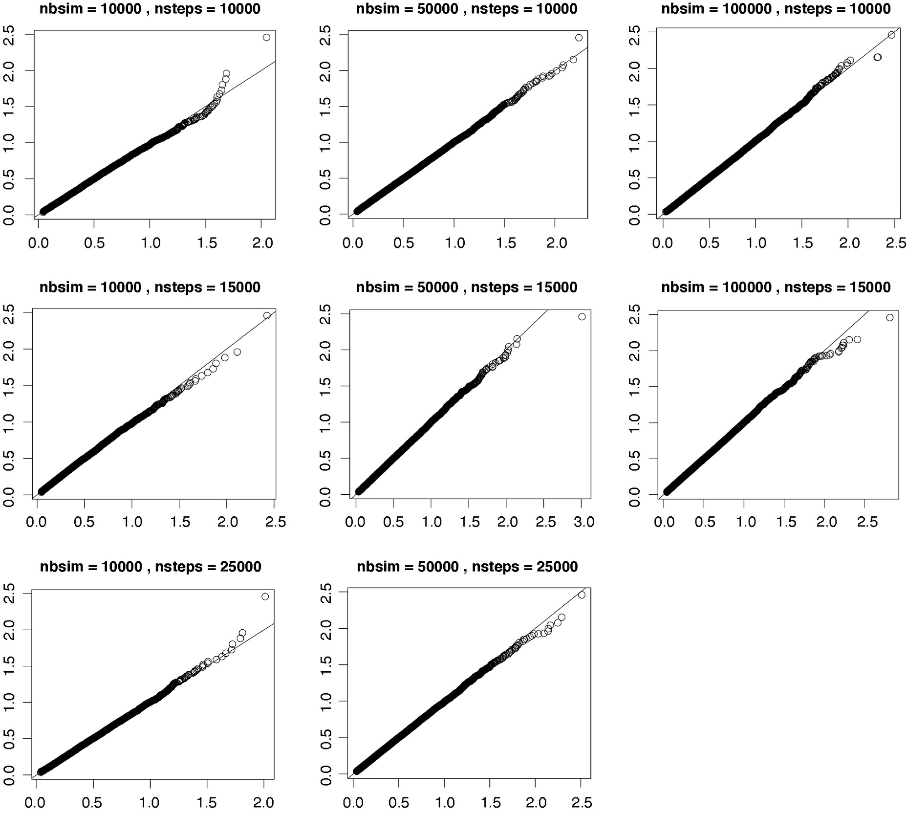
Let us now discuss the number of simulations and the discretization step for the Brownian bridge used in the simulation of the asymptotic distribution. We compare the simulated distribution function for different numbers of simulations ({1000, 10,000, 50,000, 100,000}) and different numbers of discretization steps ({10,000, 15,000, 25,000}). The sensitivity analysis is conducted for the common values for q. Figures 2–4 summarize the results for q {2, 3, 4}. The departures that are sometimes visible on the right occur in the far tail of the distribution. This is easily seen from the values of the 95th and 99th percentile of the distributions, which are equal to 0.4642337 and to 0.7457122 for q = 2, to 0.7536059 and to 1.0790407 for q = 3, and to 1.002293 and to 1.355677 for q = 4. Based on these results, performing 100,000 simulations with 10,000 discretization steps appears to be reasonable for practical applications.

Figure 2.QQ-plot for the simulated asymptotic distribution for various numbers of simulations and discretization steps for the Brownian bridge in the case q = 2. Comparisons with the asymptotic distribution obtained from 100,000 simulations and 25,000 discretization steps

Figure 3.QQ-plot for the simulated asymptotic distribution for various numbers of simulations and discretization steps for the Brownian bridge in the case q = 3. Comparisons with the asymptotic distribution obtained from 100,000 simulations and 25,000 discretization steps

Figure 4.QQ-plot for the simulated asymptotic distribution for various numbers of simulations and discretization steps for the Brownian bridge in the case q = 4. Comparisons with the asymptotic distribution obtained from 100,000 simulations and 25,000 discretization steps

5.3.2. Continuous-continuous case

Let us examine the convergence of the exact distribution towards the asymptotic distribution when both variables are continuous. To this end, we rely on the R package copula and its functions indepTestSim to compute the exact distribution for a given sample size and indepTest to compute the test statistic on a given data set. We also discuss there the number of simulations needed to obtain a stable asymptotic distribution.

Since the distribution only relies on ranks, we can simulate independent uniform random variables to assess the exact distribution under H₀. Repeating this 100,000 times allows us to simulate the exact distribution for a given sample size. Let us compute this distribution for the following sample sizes: 100, 200, 1000, 2000. We compare these exact distributions with the asymptotic distribution using a QQ-plot as depicted on Figure 5.

Figure 5.QQ-plot between the exact distributions for various sample sizes and the asymptotic distribution

We also analyze the sensitivity of the asymptotic distribution function to the number of simulations. Some quantiles for various numbers of simulations are given in Table 5. We can see there that as soon as the sample size reaches 250, the simulated quantiles stabilize after 10,000 simulations.

5.4. Results of the independence tests

We now apply the tests described in Sections 2–4: as explained in the previous sections, we use the likelihood ratio test, the discrete-discrete case, the Cramer–von Mises test in the discrete-continuous case, and the independence copula test in the continuous-continuous case. In Table 6 we display the p-values for each test. In the discrete-discrete case, we use the function likelihood.test from the R package Deducer. In the continuous-discrete case, the asymptotic distribution of the statistic W_n under the independence hypothesis was obtained using 100,000 simulations and 10,000 discretization steps for the Brownian bridge. This can be done in R using the following commands:

library(Sim.DiffProc)
mc-100000 #Number of simulations
T-matrix(nrow=mc,ncol=1)
# q = number of possible values for X
for (k in 1:mc)
{
simbbridge-BB(N=10000,M=q-1,x0=0,y=0,t0=0,T=1);
T[k, 1]-sum(rowSums(simbbridge^2))/10000;
}

Once the statistic has been computed on the data set, the p-values are found using the quantile function. In the continuous-continuous case, the asymptotic distribution of the statistic I_n was computed using 100,000 simulations. The distribution can be simulated using the formula from Section 4.3, and, as discussed in Table 5, by restricting the sum over the first 100 × 100 terms. Low p-values mean that independence is rejected. For the binary variable I, independence is rejected for most of the explanatory variables at all the usual confidence levels, with the exception of Use. Considering the response variable N*⁺, independence with respect to the explanatory variables is less often rejected. Hence, we observe that most variables could be used to explain whether at least one claim has been recorded, while fewer variables seem to be relevant to explain the number of claims, knowing that at least one claim has been registered. This would suggest to use a zero-modified count regression model as it enables to enter different scores for the probability mass at zero and for the probabilities assigned to positive integers. Nevertheless, let us mention that fewer data points are available to test the independence of the explanatory variables to N*⁺ compared to I, which may impact on the power of the test. Notice that the added uniform noise to the variables AgePh and AgeCar does not alter the results. P-values remain very similar and the conclusion of the tests are unaltered when other uniform noises are added.

Because of the large sample size (about 160,000 policies, among which about 18,000 produced claims) we could have expected that the independence tests would have been less effective since most variables would have a low p-value. The results reported in Table 6, however, show that some p-values remain high, suggesting that the corresponding explanatory variables can be excluded from the analysis, despite the large sample size.

Considering the average cost per claim \(\overline{S}\), we detect an effect of all covariates except Fuel that turns out to only impact the variable I. The effect of Use is moderate, with a p-value in the grey zone 5%–10%.

In this simple example, we see that some explanatory variables can be excluded from the very beginning, as they do not appear to be correlated with the responses. Reducing the number of explanatory variables to be considered in the multivariate regression analysis helps the actuary to simplify the interpretation of the results.

For the sake of comparison, we also run an ordered logistic regression using the function polr from package MASS in R to explain N^*+ with the covariate Fuel and a gamma regression to explain the average cost of claims \(\overline{S}\). In both cases, Fuel was found to be unsignificant (p-values of 0.7628 and 0.2561), so that we reach the same conclusion than those obtained with the tests presented in this paper. Notice that to obtain the p-value in the ordered logistic regression a likelihood ratio test between the model with only the intercept and the model with the variable Fuel was run. A logistic regression was also run between I and Fuel. A deviance test to compare both models (one with explanatory variable Fuel, and one with only an intercept) yielded similar results to those reported in Table 6: p-value below 2.2 × 10^–16, deviance of 136.38.

Even if both approaches agree on these examples, we believe that the results of Table 6 are more reliable in that they are fully nonparametric. The conclusions drawn from the logistic or gamma regressions could be distorted by an inappropriate choice of link function and/or distributional assumption.

Notice that the variable Region considered in our example has been considerably simplified, with only nine levels resulting from grouping according to the first digits of the ZIP code. Using the exact geographical location as reflected by ZIP codes would mean distinguishing more than 600 districts in Belgium. We must acknowledge that the tests proposed in the present paper cannot deal with such a multi-level risk factor. Credibility mechanisms, or mixed models, can be used to deal with such factors at a later stage of the analysis, as explained for instance in Ohlsson and Johansson (2010).

6. Discussion

In this paper, we have presented an approach to assess whether a covariate X influences a response Y. This approach enables actuaries to treat in a consistent way all the cases arising from the possible formats of X and Y (even if the underlying techniques differ from one case to another). Indeed, we have provided actuaries with nonparametric tests for independence, appropriate to each format and that come up with corresponding p-values. These independence tests can be applied routinely and the results are obtained in just a few seconds on a whole set of possible covariates. This is in contrast with other variable selection methods, such as random forests, which can take more time to be performed, as well as with other approaches (such as Lasso) which require careful selection of tuning parameters by cross-validation. Of course, the methods described in this paper do not replace these multivariate tools but only aim to reduce the number of predictors to be considered at later stages of the analysis. This can be particularly useful when GLMs are used, for instance. The conclusions of the independence tests may also guide the choice of the model, suggesting a specific score to capture the influence of the risk factors on the zero-claim probability.

The main discovery of our numerical illustrations is that some risk factors appear to influence the indicator I but not N*⁺, and vice versa. This suggests that the actuary resorts to zero-modified regression models, such as those studied in Boucher, Denuit, and Guillen (2007).

Notice that we have not discussed interactions. When these effects are included in the model by means of additional covariates, the proposed testing procedures can be applied to these new variables. For instance, when both explanatory variables are discrete, the presented likelihood ratio test can be performed on the variable which consists in the Cartesian product of both explanatory discrete variables. Also, if the variable of interest is discrete and only one of the explanatory variable is discrete, then the test from Section 3 can be used to assess the interaction.

Let us also mention that all the formulas rely on values of n, so that observations are not weighted by exposure. All independence tests have been developed for independent and identically distributed bivariate observations so that unequal risk exposures cannot be taken into account. As the tests are intended to be used in a preliminary stage, to perform a first selection of potential risk factors, this does not seem to be an issue. In the portfolio under study, most policyholders were present for the whole year. As long as the distribution of exposures does not vary according to the levels of the explanatory variables, unequal exposures should not affect the conclusions. In some cases where such a situation may occur (for instance, very young drivers who often spend less than one year in the portfolio after getting their license), this point may require further attention.

The presented methods, however, do not allow us to classify the variables by the strength of their dependence to the response because smaller p-values do not necessarily reveal stronger dependence. In order to measure the degree of association between the response Y and a risk factor X for which independence has been rejected, one can refer to association measures. One possibility is the comparison of the variability of the pure premium E[Y|X] with the variability of the loss variable Y. Specifically, we start from the well-known decomposition of the variance formula

\[ \mathrm{V}[Y]=\mathrm{E}[\mathrm{V}[Y \mid X]]+\mathrm{V}[\mathrm{E}[Y \mid X]] . \]

In case of independence, the last term is equal to zero, since E[Y|X] is constant, while in case of perfect association, i.e., when Y = f(X) for some measurable function f, the first term is equal to zero, since there is no uncertainty left when knowing X. So, the following reduction in variability

\[ \frac{\mathrm{V}[Y]-\mathrm{V}[\mathrm{E}[Y \mid X]]}{\mathrm{V}[Y]} \]

measures by how much the variability of Y is reduced by knowing X. Therefore, we can measure the degree of association between X and Y by the ratio

\[ \rho=\frac{\mathrm{V}[\mathrm{E}[Y \mid X]]}{\mathrm{V}[Y]} \in[0,1] . \tag{6.1} \]

The ratio ρ is the part of the total variance supported by the policyholders. See, e.g., De Wit and Van Eeghen (1984) for more details. The association measure (6.1) is currently under study.

Acknowledgements

We thank the editor and the four anonymous referees for their careful reading and for the numerous suggestions that greatly helped us to improve an earlier version of this text.

The authors gratefully acknowledge the financial support from the contract “Projet d’Actions de Recherche Concertées” No 12/17-045 of the “Communauté française de Belgique,” granted by the “Académie universitaire Louvain.” Also, the financial support of the AXA Research Fund through the JRI project “Actuarial dynamic approach of customer in P&C” is gratefully acknowledged. We thank our colleagues from AXA Belgium, especially Mathieu Lambert, Alexis Platteau and Stanislas Roth for interesting discussions that greatly contributed to the success of this research project.