Back-Testing the ODP Bootstrap of the Paid Chain-Ladder Model with Actual Historical Claims Data

1. Introduction

Reserve risk is one of the largest risks that non-life insurers face. A study done by Best (2010) identified deficient loss reserves as the most common cause of impairment^[1] for the U.S. non-life industry in the last 41 years. It accounted for approximately 40% of impairments in that period. This, as well as encouragement from Solvency II regulation in Europe, has resulted in the growing popularity of the estimation of reserve distributions.

The over-dispersed Poisson (ODP) bootstrap of the chain-ladder method, as described in England and Verrall (2002) is one of the most popular methods used to obtain reserve distributions.^[2] In the rest of this paper, we will simply refer to this as the “bootstrap model.”

Before relying on a method to estimate capital adequacy, it is important to know whether the method “works.” That is, is there really a 10% chance of falling above the method’s estimated 90th percentile? There have been many papers on different ways to estimate reserve risk, but very few papers on testing whether these methods work, and even fewer of these papers test the methods using real (as opposed to simulated) data.

In this paper, we test if the model works by back-testing the bootstrap model using real data spanning three decades on hundreds of companies. This paper differs from other papers on this topic to date because:

• We use real data, rather than simulated data.

• We test the reserve distribution in total—the sum of all future payments, not just the next calendar year’s payments.

• We test the distribution over many time periods—this is important due to the existence of the reserving cycle.

• We test multiple lines of business.

We suspect that other papers have not attempted this due to a lack of data of sufficient depth and breadth. In contrast, we have access to an extensive, cleaned U.S. annual statement database, as described in Section 3.

2. Summary of existing papers

There have been a limited number of papers on the back-testing of reserve risk methods. Below are summaries of three such papers.

2.1. General Insurance Reserving Oversight Committee (2007) and (2008)

The General Insurance Reserving Oversight Committee, under the Institute of Actuaries in the U.K., published two papers in 2007 and 2008, detailing their testing of the Mack and the ODP bootstrap models. They tested these models with simulated data that complied with all the assumptions under each model. The ODP bootstrap model tested by the committee is the same as the bootstrap of the paid chain-ladder model being tested in this paper, as detailed in England and Verrall (2002). The results showed that even under these ideal conditions, the probabilities of extreme results could be understated using the Mack and the ODP bootstrap models. The simulated data exceeded the ODP bootstrap model’s 99th percentile between 1% and 4% of the time. The 1% result was from more stable loss triangles. The simulated data exceeded the Mack model’s 99th percentile between 2% and 8% of the time.

The Committee also tested a Bayesian model (as detailed in G. G. Meyers (2007)) with U.K. motor data (not simulated data). The test fitted the model on the data, excluding the most recent diagonal, and the simulated distributions of the next diagonal are compared to the actual diagonal. The model allows for the error in parameter selection that can help overcome some of the underestimation of risk seen in the Mack and ODP bootstrap models. However, “it is no guarantee of correctly predicting the underlying distribution.”

2.2. “The Retrospective Testing of Stochastic Loss Reserve Models” by G. Meyers and Shi (2011)

This paper back-tests the ODP bootstrap model as well as a hierarchical Bayesian model, using commercial auto liability data from U.S. annual statements for reserves as of December 2007. Two tests were performed. The first was to test the modeled distribution of each projected incremental loss for a single insurer. The second was to test the modeled distribution of the total reserve for many insurers, which is very similar to the test in this paper, however limited to only one time period (reserves as of December 2007). The authors conclude: “[T]here might be environmental changes that no single model can identify. If this continues to hold, the actuarial profession cannot rely solely on stochastic loss reserve models to manage its reserve risk. We need to develop other risk management strategies that do deal with unforeseen environmental changes.”

3. Data

The data used for the back-testing are from the research database developed by Risk Lighthouse LLC and Guy Carpenter. In the U.S., (re)insurers file annual statements each year as of December 31. The research database contains annual statement data from the 21 statement years 1989 to 2009.^[3] Within the annual statement is a Schedule P that, net of reinsurance, for each line of business, provides the following:

• A paid loss triangle by development year for the last 10 accident years.

• Booked ultimate loss triangle by year of evaluation, for the last 10 accident years, showing how the booked ultimate loss has moved over time.

• Earned premium for the last 10 accident years.

Risk Lighthouse has cleaned the research database by

• Re-grouping all historical results to the current company grouping as of December 31, 2009, to account for the mergers and acquisitions activities over the past 31 years;

• Restating historical data (e.g., under new regulations a previous transaction does not meet the test of risk transfer and must be treated as deposit accounting);

• Cleaning obvious data errors, such as reporting the number not in thousands but in real dollars.

For the purposes of our back-testing study, we refined our data as follows:

• We used company groups rather than individual companies since a subsidiary company cedes business to the parent company or sister companies and receives its percentage share of the pooled business.

• To ensure we had a reasonable quantity of data to apply the bootstrap model, we used up to 100 of the largest company groups for each line of business. For each line we began with the largest^[4] 100 company groups and removed those with experience that cannot be modeled due to size or consistency (some companies are missing random pieces of data). The resulting number of companies ranges from a high of 78 companies for Private Passenger Auto to a low of 21 companies for Medical Professional Liability.^[5]

• We used losses net of reinsurance, rather than gross. As a practical issue, the paid loss triangles are only reported net of reinsurance, and this also avoids the inter-company pooling and possible double counting issue of studying gross data for company groups. Additionally, loss triangles gross of reinsurance can be created, but this data covers around half of the time span of the data net of reinsurance.

• We concentrated on the following lines of business:

  1. Homeowners (HO)

  2. Private Passenger Auto (PPA)

  3. Commercial Auto Liability (CAL)

  4. Workers Compensation (WC)

  5. Commercial Multi Peril (CMP)

  6. Medical Professional Liability—Occurrence and Claims Made (MPL)

  7. Other Liability—Occurrence and Claims Made (OL)

The Other Liability and Medical Professional Liability lines have only been split into Occurrence and Other Liability subsegments since 1993. Therefore, to maintain consistency pre- and post-1993, we have combined the two subsegments for these lines.

4. The method being tested

We are testing the reserve distribution created using the ODP bootstrap of the paid chain-ladder method, or simply the “bootstrap model” as described in Appendix 3 of England and Verrall (2002). We feel it is the most commonly used version of the model. How it specifically applies in our test is outlined below, and the steps with a numerical example are shown in Appendix A.

1. Take a paid loss and ALAE, 10 accident year by 10 development year triangle.

2. Calculate the all-year volume-weighted average age-to-age factors.

3. Estimate a fitted triangle by first taking the cumulative paid loss and ALAE to date from (1).

4. Estimate the fitted historical cumulative paid loss and ALAE by using (2) to undevelop (3).

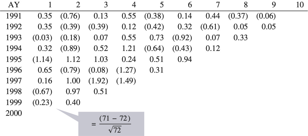
5. Calculate the unscaled Pearson residuals, r_p (from England and Verrall (1999)):

   $$r_{p}=\frac{C-m}{\sqrt{m}}$$

   where

   1. C = incremental actual loss from step (1) and

   2. m = incremental fitted loss from step (4).

6. Calculate the degrees of freedom and the scale parameter:

   $$D o F=n-p$$

   where

   1. DoF = degrees of freedom

   2. n = number of incremental loss and ALAE data points in the triangle in step 1, and

   3. p = number of parameters in the paid chain-ladder model (in this case, 10 accident year parameters and 9 development year parameters).

      $$\text {Scale Parameter}=\frac{\sum r_{p}^{2}}{D o F}.$$

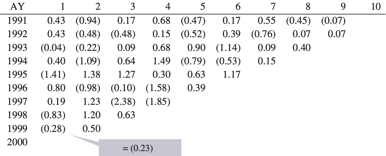
7. Adjust the unscaled Pearson residuals (r_p) calculated in step (5):

   $$r_{p}^{a d j}=\sqrt{\frac{n}{D o F}} \times r_{p}.$$

8. Sample from the adjusted Pearson residuals r_p^adj in step (7), with replacement.

9. Calculate the triangle of sampled incremental loss C.

   $$C=m+r_{p}^{a d j} \sqrt{m}.$$

10. Using the sampled triangle created in (9), project the future paid loss and ALAE using the paid chain-ladder method.

11. Include process variance by simulating each incremental future loss and ALAE from a Gamma distribution with the following:

    $$\begin{array}{c} \text { mean }=\text { projected incremental loss in step }(10), \text { and } \\ \text { variance }=\text { mean } \times \text { scale parameter from step }(6). \end{array}$$

    We assume that each future incremental loss is independent from each other. Note that theoretically we assume an over-dispersed Poisson distribution; however, we are using the Gamma distribution as a close approximation.

12. Estimate the unpaid loss and ALAE by taking a sum of the future incremental losses from step (10).

13. Repeat steps (8) to (12) (in our case, 10,000 times to produce 10,000 unpaid loss and ALAE estimates resulting in a distribution).

It is important to note that we are only testing the distribution of the loss and ALAE that is unpaid in the first 10 development years. This is to avoid the complications in modeling a tail factor.

5. Back-testing

5.1. Back-testing Accident Year 2000 as of December 2009

The steps in our back-testing are detailed below. First, we detail the steps for one insurer at one time period and then expand this to multiple insurers over many time periods.

1. Create a distribution of the unpaid loss and ALAE by using the bootstrap model as of December 2000, as detailed in section 4, using Schedule P paid loss and ALAE data for a particular company A’s homeowners book of business.

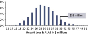
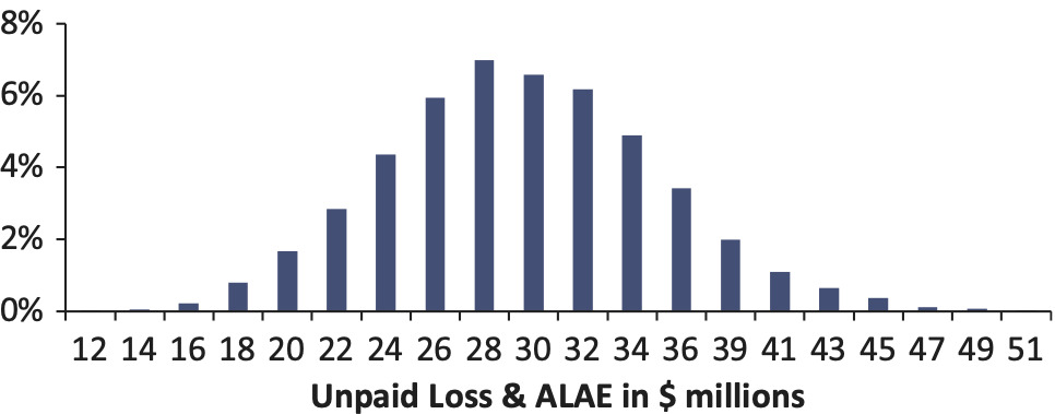
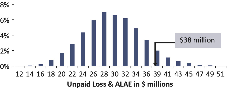
2. Isolate the distribution of unpaid loss and ALAE for the single accident year 2000, as shown in Figure 1. We do this so that we can test as many time periods as possible.

Figure 1.Company A’s distribution of unpaid loss & ALAE, net of reinsurance as of 12/2000

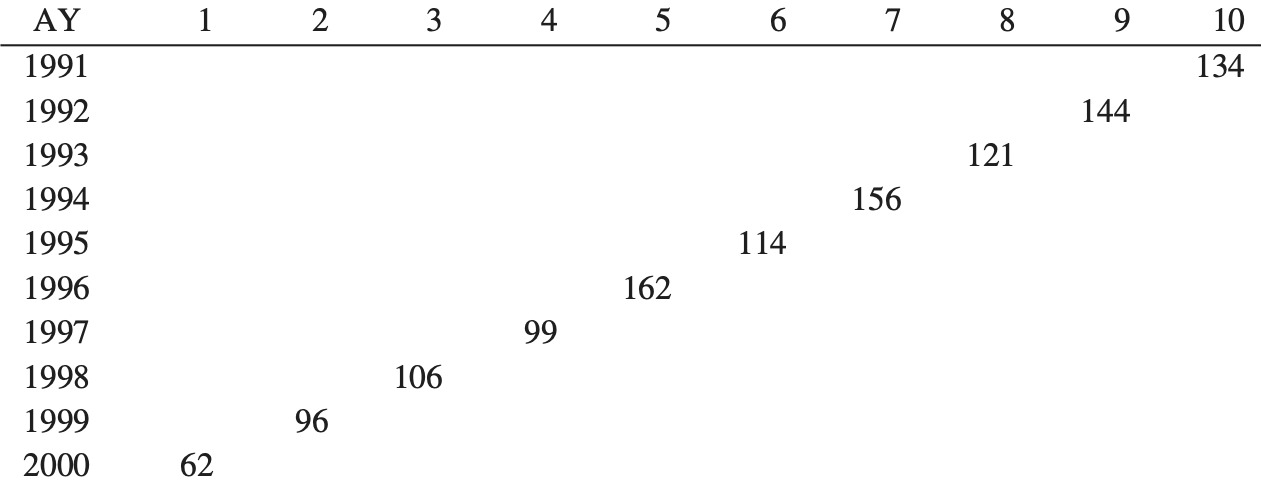
3. The unpaid loss and ALAE is an estimate of the cost of future payments. Eventually, we will know how much the actual payments cost. In this case, the actual payments made total $38 million^[6] (sum of the payments for accident year 2000 from development years 2 to 10). We call this the “actual” unpaid—what the reserve should have been, with perfect hindsight. Figure 2 shows that this falls at the 91st percentile of the original distribution.

Figure 2.Company A’s distribution of unpaid loss and ALAE, net of reinsurance as of 12/2000, for accident year 2000

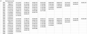
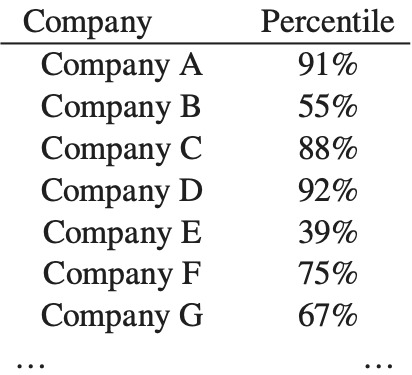
4. We can repeat steps 1 to 3 for another 74 companies. Some of the percentiles for these companies are listed in Figure 3.

Figure 3.Percentile where the actual unpaid falls in the distribution created as of 12/2000, by company

5.1.1. Results

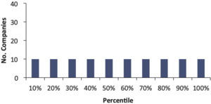
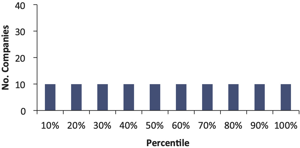
If the bootstrap model gives an accurate indication of the probability of the actual outcome, we should find a uniform distribution of these 75 percentiles. For example, the 90th percentile is a number that the insurer expects to exceed 10% of the time (that is the definition of the 90th percentile). Therefore, we should find 10% of the companies have an actual outcome that falls above the 90th percentile. And similarly, there should be a 10% chance that the actual unpaid falls in the 80th to 90th percentile and so on. That is, ideally we should see Figure 4 when we plot these percentiles.

Figure 4.Ideal histogram of percentiles

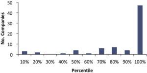
When we plot the percentiles in Figure 3, what we actually see is shown in Figure 5.

Figure 5.Histogram of percentiles for homeowners as of 12/2000, for the accident year 2000

This shows that 46 out of 75 companies had actual unpaid amounts that fell above the 90th percentile of the original distributions created as of 12/2000. For 46 out of 75 companies, the reserve was much higher than the mean of the paid chain-ladder bootstrap.

5.2. Back-testing Accident Year 1996 as of December 2009

The test can be repeated at another time period—instead of December 2000, we can try December 1996. That is, we repeat steps 1 to 4, but this time, we are creating distributions for the reserves for accident year 1996 only, for 76 companies as of December 1996.

5.2.1. Results

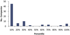
The histogram of the resulting percentiles is shown in Figure 6.

Figure 6.Histogram of percentiles for homeowners as of 12/1996, for accident year 1996

In this case, 45 out of 76 companies had actual unpaid amounts that fell below the 10th percentile of the original distributions created as of 12/1996. For 45 out of 76 companies, the reserve was much lower than expected by the paid chain-ladder bootstrap. This is the opposite of the result seen as of 12/2000.

These results mirror the reserve cycle, to be discussed in greater detail later, where most insurers are either under- or over-reserved at each point in time. At any one point in time, the reserve is estimated with what is currently known. As the future unfolds and the claims are actually paid, some systemic effect can cause the claims environment to move away from the historical experience, causing most insurers to be either under- or over-reserved. For example, at the time of writing (2012) inflation has been historically low, and actuaries set their current reserves in this environment. If, as the future unfolds, claims inflation increases unexpectedly, then the reserves for most insurers will be deficient, similar to what is seen in Figure 5.

Therefore, testing one time period at a time may not result in a uniform distribution of percentiles. However, if many time periods are tested, and all the percentiles are plotted in one histogram, this may result in a uniform distribution.

5.3. Back-testing multiple periods

For this test, repeat steps 1 to 4 in section 5.1, each time estimating the reserve distribution as of 12/1989, 12/1990, 12/1991 . . . to 12/2002. Note that at the time of testing, we only had access to data as of 12/2009. The actual unpaid for accident year 2002 should be the sum of the payments for that accident year from the 2nd to the 10th development year. However, as of 12/2009 we only have payments from the 2nd to the 8th development period. The remaining payments had to be estimated. A similar issue exists for the test as of 12/2001. We use the average of company’s accident year 1998 to 2000, 96th to 120th development factors to estimate the remaining payments.

5.3.1. Results

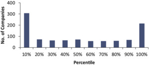
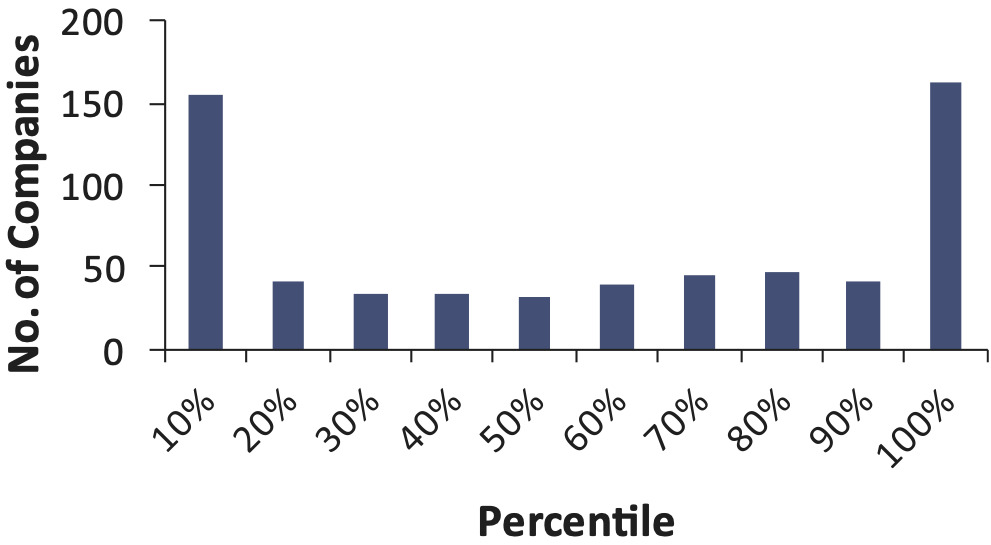
The test for an average of 74 companies for 14 accident years results in 1,038 percentiles, shown in a histogram in Figure 7.

Figure 7.Histogram of percentiles for Homeowners as of 12/1989, 12/1990 . . . and 12/2002

Figure 7 shows that, around 20% of the time, the actual unpaid is above the 90th percentile of the bootstrap distribution, and 30% of the time the actual unpaid is below the 10th percentile of the distribution. When you tell management the 90th percentile of your reserves, this is a number they expect the reserve to exceed 10% of the time. Instead, when using the bootstrap model, we find that companies have exceeded the modeled 90th percentile 20% of the time. In this test, the bootstrap model appears to be underestimating reserve risk.

5.4. Back-testing of other lines of business

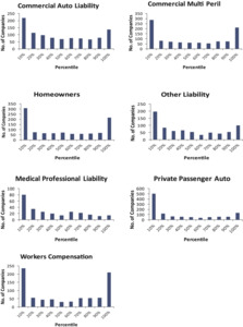
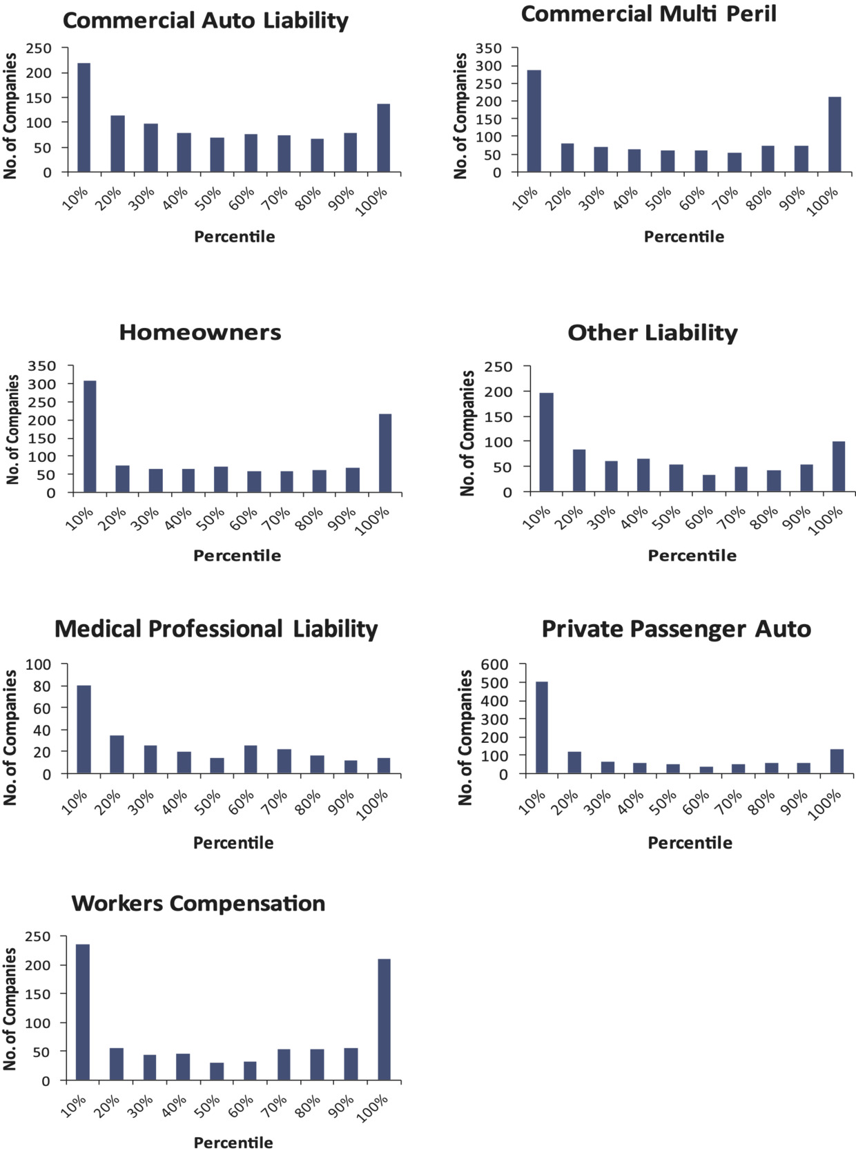
The test can be repeated for the other lines of business. When this is done, the results are shown in Figure 8.

Figure 8.Histogram of percentiles as of 12/1989, 12/1990 . . . and 12/2002

The histograms do not follow a uniform distribution. In this test, for most of these lines of business, using the bootstrap model has produced distributions that underestimate reserve risk. However, for medical professional liability and private passenger auto in particular, it appears that the paid chain-ladder method is producing reserve estimates that are biased high.

6. Analysis of the results

A reserve distribution is a measure of how the actual unpaid loss may deviate from the best estimate. By applying the ODP bootstrap to the paid chain-ladder method, we can get such a reserve distribution around a paid chain-ladder best estimate.

However, it is rare to rely solely on this method to determine an actuarial central reserve estimate. For better or worse, it is common practice for actuaries to estimate a distribution by using a similar ODP bootstrap of the chain-ladder method outlined here, and then “shift” this distribution by multiplication so that the mean is the same as an actuarial best estimate reserve or booked reserve.

We do not condone this practice, but it is so common that a natural question is whether the “shifting” of the distributions produced in our back-testing would result in a more uniform distribution. Booked reserve estimates use more sophisticated methods than the paid chain-ladder model, and therefore may be more accurate, so the width of the distributions being produced in this study may be perfectly suitable. If we had used the booked reserve, then we may not have seen the under- and over-reserving in the December 2000 and December 1996 results, respectively

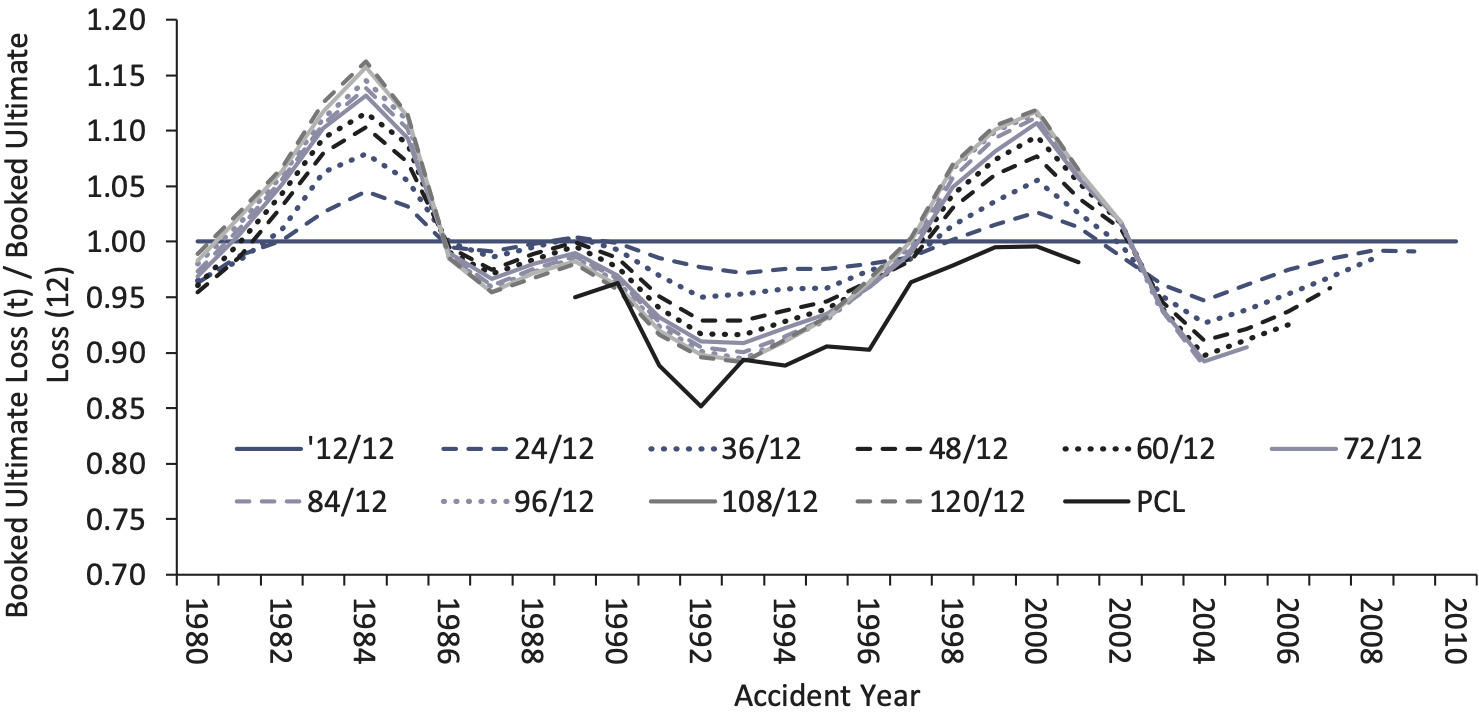
In reality, the industry does under- and over-reserve, sometimes significantly. In comparison to the paid chain-ladder method, the industry is sometimes better or worse at estimating the true unpaid loss. In Figure 9, we show the booked ultimate loss at 12, 24, 36 . . . and 120 months of evaluation, divided by the booked ultimate loss at the 12-month evaluation, for the U.S. industry, in aggregate for the seven lines of business tested in this paper.

Figure 9.Booked ultimate loss at t months of evaluation/booked ultimate loss at 12 months of evaluation, in aggregate for the industry for seven lines of business, net of reinsurance

The “PCL” line on this graph shows the cumulative paid loss and ALAE at 120 months of evaluation divided by the PCL estimate at 12 months of evaluation (using an all-year weighted average on an industry 10 accident year triangle by line of business and excluding a tail factor).

For example, for accident year 2000, the booked ultimate loss estimate as of 12/2009 ended up 12% higher than the initial booked ultimate loss as of 12/2000. In contrast, the paid chain-ladder estimate of the ultimate loss as of 12/2009 was the same as the estimate as of 12/2000—that is, the paid chain-ladder reserve estimate as of 12/2000 was more accurate than the booked reserve.^[7]

The cycle in Figure 9 is for all lines of business. However, the main driver of the cycle is the long-tailed casualty lines like Other Liability, Workers Compensation and Medical Professional Liability. They all individually have a strong cyclical pattern.

Shifting a distribution around another mean is not a sound practice. Even ignoring this, we did not feel that shifting the mean to equal the booked reserve at the time would have materially changed the broad result of our back-testing.

6.1. Why are we seeing these results?

In an Institute of Actuaries of Australia report, (IAAust 2008) the sources of uncertainty in a reserve estimate are grouped into two parts: independent risk and systemic risk.

1. Independent risk = “risks arising due to the randomness inherent in the insurance process.”

2. Systemic risk = a risk that affects a whole system, “risks that are potentially common across valuation classes or claim groups” (IAAust 2008). Even if the model is accurately reflecting the claims process today, future trends in claims experience may move systematically away from what was experienced in the past—for example, unexpected changes in inflation, unexpected tort reform, or unexpected changes in legislation.

They state that the traditional quantitative techniques, such as bootstrapping, are better at analyzing independent risk but aren’t able to adequately capture systemic risk. This is because, even if there are past systemic episodes in the data, “a good stochastic model will fit the past data well and, in doing so, fit away most past systemic episodes of risk . . . leaving behind largely random sources of uncertainty” (IAAust 2008).

The distributions produced in this paper using the bootstrap model may be underestimating reserve risk because they only capture independent risk, not systemic risk.

7. Possible adjustments to the method

If the ODP bootstrap of the paid chain-ladder method is producing distributions that underestimate the true reserve risk, then what adjustments can be made so that it more accurately captures the risk?

7.1. Commonly used possible adjustments

7.1.1. Bootstrapping the incurred chain-ladder method

Using the method outlined in this paper on incurred loss and ALAE data instead of paid loss and ALAE data produces reserve distributions with a smaller variance. This is understandable if you assume that the case reserves provide additional information about the true cost of future payments. We back-tested the incurred bootstrap model for the Workers Compensation line of business. The process was the same as for the paid bootstrap model, but incurred loss and ALAE was substituted for the paid loss and ALAE data, resulting in distributions of IBNR. The resulting percentiles are in Figure 10.

Figure 10.Histogram of percentiles for workers compensation as of 12/1989, 12/1990 . . . 12/2002 based on incurred loss and ALAE

From Figure 10, it appears that the incurred bootstrap model is also underestimating the risk of falling in these extreme percentiles.

7.1.2. Using more historical years of paid loss and ALAE data

Our back-testing used paid loss and ALAE triangles with 10 historical accident and development years. A loss triangle with more historical accident years may result in a wider distribution.

We applied the bootstrap model on 20 accident year × 10 development year homeowners paid loss and ALAE triangles, but this resulted in distributions that sometimes had more and sometimes had less variability than the original distributions from the 10 × 10-year datasets.

7.1.3. Making other adjustments

There are other additions to the bootstrap model that we have not considered here, and can be areas of further study:

• Parametric bootstrapping. It is possible to simulate the accident year and development year parameters from a multivariate normal distribution using a generalized linear model, which closely follows the structure of the ODP bootstrap of the paid chain-ladder model. This is commonly called parametric bootstrapping. Re-sampling the residuals, as outlined in section 3, may be limiting, and simulating from a normal distribution may result in wider reserve distributions.

• Hat matrix. The hat matrix can be applied to standardize the Pearson residuals and make them identically distributed, as per Pinheiro, Andrade e Silva, and De Lourdes Centeno (2003).

• Multiple scale parameters to account for heteroskedasticity in residuals.

None of these commonly used adjustments are specifically designed to account for systemic risk. Also, the method we are testing significantly underestimates the true risk and so requires an adjustment that significantly widens the distribution. Therefore, we outline below two methods that can be applied to the bootstrap model that account for systemic risk.

7.2. Two methods to account for systemic risk

We have derived two methods to adjust the ODP bootstrap of the paid chain-ladder model so that the resulting distributions of unpaid loss and ALAE describe the true reserve risk—that is, it passes our back-testing, so that, for example, 10% of the time the actual unpaid falls above the 90th percentile of our estimated distribution. These two methods are explicitly attempting to model systemic risk—the risk that the future claims environment is different from the past.

The two methods are:

1. The systemic risk distribution method, and

2. Wang transform adjustment.

The two methods are based on two different assumptions. The systemic risk distribution method does not adjust the actuary’s central estimate over the reserving cycle. The Wang transform adjustment does not assume that the central estimate reserve is unbiased and tries to estimate the systemic bias of the chain-ladder method over the course of reserving cycle.

Both methods are applied and the resulting distribution is back-tested again.

7.2.1. Systemic risk distribution method

As outlined in section 6.1, reserve risk can be broken down into two parts: (1) independent risk and (2) systemic risk. We believe that the bootstrap model only measures independent risk, not systemic risk. Systemic risk affects a whole system, like the market of insurers. It includes risks such as unexpected changes in inflation and unexpected changes in tort reform—in short, the risk that the future claims environment could be different from the past.

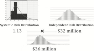
In this method, we estimate a benchmark systemic risk distribution by line of business, and combine this with the independent risk distribution (from the bootstrap model) to obtain the total reserve risk distribution. To combine the distributions we assume that they are independent from each other, and take one simulation from the systemic risk distribution and multiply this by one simulation from the independent risk distribution, and repeat for all 10,000 (or more) iterations.

Each of the outcomes from the systemic risk distribution, such as the 1.13 in Figure 11, can be thought of as a systemic risk factor. We can calculate historical systemic risk factors for each year and for each company by the following procedure:

1. Take the mean of the bootstrap model’s reserve distribution for each company, as of 12/1989 for accident year 1989.

2. Calculate what the reserve should have been for accident year 1989, as of 12/1989 (= the ultimate loss and ALAE as of 12/1998 less the paid as of 12/1989).

3. The systemic risk factor = (2)/(1).

4. Repeat 1 to 3 as of 12/1990, 12/1991, . . . . to 12/2002.

Figure 11.Example of one iteration of the systemic risk distribution adjustment

The systemic risk benchmark distribution is estimated by fitting a distribution to the historical systemic risk factors. Through a curve-fitting exercise, we found that a Gamma distribution was the best candidate to model systemic risk, with differing parameters by line of business. This results in uniform distributions of percentiles when the method outlined above is back-tested, as shown in Figure 12.

Figure 12.Histogram of percentiles as of 12/1989, 12/1990 . . . to 12/2002

Admittedly, the fitted systemic risk distribution may differ depending on the back-testing period. However, we took care to span a time period that incorporated one upwards and one downwards period of the reserve cycle, in an attempt to not bias the results.

As an example, for Homeowners, the systemic risk distribution is a gamma distribution with a mean of 0.98 and a standard deviation of 19%. Note that this is intended to adjust the distribution of the reserve for a single accident year at 12 months of evaluation.

Systemic risk has its roots in the reserving cycle and underwriting cycle. Indeed, there are documented evidences of the linkage between reserving cycle and underwriting cycle. Archer-Lock et al. (2003) discussed the reserving cycle in the U.K. The authors conclude that the mechanical application of traditional actuarial reserving methods may be one of the causes for the reserve cycle. In particular, the underwriting cycle may distort claims development patterns and that premium rates indices may understate the magnitude of the cycle. The Wang transform adjustment is an alternative systemic risk adjustment that explicitly accounts for the reserve cycle.

7.2.2. Wang-transform adjustment

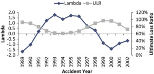
The Wang transform adjustment method does not assume that the unpaid loss and ALAE estimate is unbiased and tries to estimate the systemic bias over the course of reserving cycle. The reserving cycle shown in Figure 13 is an interesting phenomenon that indicates that reserve risk is cyclical, and the Wang transform adjustment method tries to capture this “systemic” bias.

Figure 13.Chain-ladder method back-testing error versus (ULR-ILR) for workers compensation

We use the workers compensation line of business for illustration. The data used in back-testing is the workers compensation aggregated industry data net incurred loss and ALAE. A series of back-tests (these back-tests are different from the test in section 4) are done using the chain-ladder method for industry loss reserve development. For accident years after 2001, we use the latest reported losses instead of the projected ultimate losses, since reported losses for those accident years are not yet fully developed.

In the following figures, which represent the entire non-life industry workers compensation line of business, Ultimate Losses (UL) stand for the 120-month incurred loss and ALAE for each accident year (AY) from the latest report year (RY), not including IBNR. Initial Losses (IL) represent the projected 120-month net incurred loss and ALAE for each AY from first report year, using the chain-ladder reserving method. Ultimate Loss Ratio (ULR) represents the ultimate booked including IBNR incurred loss and ALAE ratio for each AY and Initial Loss Ratio (ILR) represents the initial booked including IBNR incurred loss ratio for each AY. A more detailed explanation of the back-testing method is given in Appendix B.

For the workers compensation line of business, the chain-ladder reserving method has systematic errors that are highly correlated with the reserving cycle. The contemporary correlation between the estimation error (UL-IL) and the reserve development (ULR-ILR) is 0.64 for the chain-ladder method. More noticeably, the one-year lag correlation is 0.91. The estimation error leads the loss reserve development by one year.

In this study, we apply the Wang transform to enhance the loss reserve distribution created using the bootstrap of the chain-ladder method. Different from the systemic risk distribution method, the Wang transform adjustment method will first adjust the variability of the loss reserve then give each company group’s loss reserve distribution a shift, respectively.

The procedures below describe how to apply the Wang-Transform adjustment:

1. After bootstrapping each paid loss triangle with 10,000 iterations, we apply the ratio of double exponential over normal to adjust the chain-ladder reserve distribution to be wider than the original distribution. The formula is

   $$\begin{aligned} x^{*} & =(x-u) * \text { ratio }+u \\ \operatorname{ratio}(q) & =\operatorname{exponential}^{-1}(q) / \phi^{-1}(q) \end{aligned}$$

   where:

   1. $\phi$ is a normal distribution with mean 0 and standard deviation 1.

   2. Exponential stands for a double exponential distribution with density function *$f(x)=0.5 * \lambda * \mathrm{e}^{-\lambda *|x|},-\infty<x<\infty$.

   3. q is the quantile of each simulated reserve.

   4. u is the median of 10,000 simulated reserves.

   5. x is the simulated reserve.

   6. x* is the reserve after adjustment.

2. β is calculated for each company to measure the correlation between the company and industry. The method to calculate the β is

   For each AY, if the industry systemic risk factor is significantly different from one (greater than 1.01 or less than 0.99), we use an indicator of +1 if a company’s corresponding AY systemic risk ratio is in the same direction as the industry systemic risk factor, otherwise we use an indicator of −1. For example, say the industry systemic risk factor for AY 2000 is 1.122, which is greater than 1. If company A’s AY 2000 systemic risk factor is greater than 1, we assign an indicator of +1 to company A AY 2000. If company B’s AY 2000 systemic risk factor is less than 1, we assign an indicator of −1 to company B AY 2000.

   At last, for a company,

   $$\beta = \frac{\text{sum of indicators of all AYs}}{\text{count of indicators of all AYs}}.$$

   If β is less than zero, we force it to zero.

3. The Wang transform is finally applied to adjust the mean of the reserve distribution. The formula is shown below:

   $$\mathrm{F}_{2}(\mathrm{x})=\phi\left[\phi^{-1}\left(\mathrm{~F}_{1}(\mathrm{x})\right)+\beta * \lambda\right]$$

   Where:

   1. F₁(x) is reported reserve’s percentile in the reserve distribution after step 1 adjustment.

   2. Each company has its own $\beta$ value.

   3. $\phi$ is a normal distribution with mean 0 and stdev 1.

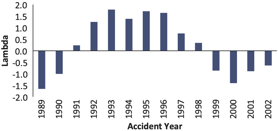
We change to result in the most uniformly distributed percentiles as measured by a chi-square test, when the adjusted reserve is back-tested. here is the fitted shift value of loss reserve distribution for each accident year.

The final $\lambda$s are shown in Figures 14 and 15.

Figure 14.Lambda for each accident year

Figure 15.Lambda vs. ULR

Comparing the fitted lambdas and the ultimate loss ratios (ULRs), we find that the loss reserve estimation error of the chain-ladder method is highly correlated with the non-life insurance market cycle. The correlation between lambda and ultimate loss ratio is −0.87.

For other lines of business, the estimated lambdas and ULRs by year are also negatively correlated, but the magnitude of correlation is not as strong as for workers compensation.

7.2.3. Areas of future research

In this paper we have demonstrated that different lambda values can be estimated at various stages of the reserve cycle. However, more research is needed in the future to illustrate the practical application of lambda in the Wang transform to the reserve cycle, and how well lambda along with the beta work for individual companies versus the industry as a whole.

In this paper, we have focused mostly on the paid loss development method. Another area of future research is to investigate the difference between using paid methods in isolation versus paid loss development methods in conjunction with case incurred loss development methods, exposure-based methods, and judgment.

Yet another area of future research is to investigate the reserve cycle illustrated in Figure 9.

8. Summary

The genesis and popularity of a reserve risk method lies in its theoretical beauty. However, as more insurers rely on actuarial estimates of reserve risk to manage capital, estimating a reserve distribution is no longer a purely theoretical exercise. Methods should be tested against real data^[8] before they can be relied upon to support the insurance industry’s solvency.

In this back-test, we see that the popular ODP bootstrap of the paid chain-ladder method is underestimating reserve risk. We believe that it is because the bootstrap model does not consider systemic risk, or, to put it another way, the risk that future trends in the claims environment—such as inflation, trends in tort reform, legislative changes, etc.—may deviate from what we saw in the past. We suggest two simple solutions to incorporate systemic risk into the reserve distribution so that the adjusted reserve distribution passes the back-test.

We hope to encourage more testing of models so that the profession has a more defensible framework for measuring risks for solvency and profitability.