Interval Estimation for Bivariate t-Copulas via Kendall’s Tau

1. Introduction

For a random vector (X, Y) with continuous marginal distributions F₁ and F₂, its copula is defined as

\[ C(x, y)=P\left(F_{1}(X) \leq x, F_{2}(Y) \leq y\right) \text { for } 0 \leq x, y \leq 1. \]

Due to its invariant property with respect to marginals, requirements in Basel III for banks and Solvency 2 for insurance companies enhance the popularity of copula models in risk management. In practice the family of elliptical copulas is arguably the most commonly employed class because it is quite easy to use in simulations with different levels of correlations. Peng (2008) used elliptical copulas to predict a rare event, and Landsman (2009) used elliptical copulas for capital allocation. Two important classes of elliptical copulas are the Gaussian copula and the t-copula. It is known that financial time series usually exhibit tail dependence, but the Gaussian copula has an asymptotically independent tail while the t-copula has an asymptotically dependent tail. Breymann, Dias, and Embrechts (2003) showed that an empirical fit of the t-copula is better than the Gaussian copula. Some recent applications and generalization of t-copulas include: Schloegl and O’Kane’s (2005) formulas for the portfolio loss distribution when a t-copula is employed; de Melo and Mendes’s (2009) option pricing applications in retirement funds using the Gaussian and t-copulas; Chan and Kroese’s (2010) t-copula model used to estimate the probability of a large portfolio loss; Manner and Segers’s (2011) study of the tails of correlation mixtures of the Gaussian and t-copulas; grouped t-copula applications were given in Chapter 5 of McNeil, Frey, and Embrechts (2005); Luo and Shevchenko (2012) and Venter et al. (2007) extended the grouped t-copula; and studies of tail dependence for multivariate t-copulas and their monotonicity were studied by Y. Chan and Li (2008).

The t-copula is an elliptical copula defined as

\[ \begin{aligned} C(u, v ; \rho, v)= & \int_{-\infty}^{5(u)} \int_{-\infty}^{\pi(v)} \frac{1}{2 \pi\left(1-\rho^{2}\right)^{1 / 2}} \\ & \left\{1+\frac{x^{2}-2 \rho x y+y^{2}}{v\left(1-\rho^{2}\right)}\right\}^{-(v+2) / 2} d y d x, \end{aligned} \tag{1.1} \]

where ν > 0 is the number of degrees of freedom, ρ ∈ [−1, 1] is the linear correlation coefficient, t_ν is the distribution function of a t-distribution with ν degrees of freedom and t_ν⁻ denotes the generalized inverse function of t_ν. When ν = 1, the t-copula is also called the Cauchy copula.

In order to fit the t-copula to a random sample (X₁, Y₁), . . . , (X_n, Y_n), one has to estimate the unknown parameters ρ and ν first. A popular estimation procedure for fitting a parametric copula is the pseudo maximum likelihood estimate (MLE) proposed by Genest, Ghoudi, and Rivest (1995). Although, generally speaking, the pseudo MLE is efficient, its computation becomes a serious issue when applied to t-copulas especially with a large dimension. A more practical method to estimate ρ uses Kendall’s tau, defined as

\[ \begin{aligned} \tau & =\mathrm{E}\left(\operatorname{sign}\left(\left(X_{1}-X_{2}\right)\left(Y_{1}-Y_{2}\right)\right)\right) \\ & =4 \int_{0}^{1} \int_{0}^{1} C\left(u_{1}, u_{2}\right) d C\left(u_{1}, u_{2}\right)-1 . \end{aligned} \]

It is known that τ and ρ have a simple relationship,

\[ \rho=\sin (\pi \tau / 2) . \]

By noting this relationship, Lindskog, McNeil, and Schmock (2003) proposed to first estimate ρ by

\[\begin{array}{c} \hat{\rho}=\sin (\pi \hat{\tau} / 2),\\ \text{where } \hat{\tau}=\frac{2}{n(n-1)} \sum_{1 \leq i<j s n} \operatorname{sign}\left(\left(X_{i}-X_{j}\right)\left(Y_{i}-Y_{j}\right)\right),\end{array} \]

and then to estimate ν by maximizing the pseudo likelihood function

\[ \prod_{i=1}^{n} c\left(F_{n 1}\left(X_{i}\right), F_{n 2}\left(Y_{i}\right) ; \hat{\rho}, v\right), \]

where \(c(u, v ; \rho, v)=\frac{\partial^{2}}{\partial u \partial v} C(u, v ; \rho, v)\) is the density of the t-copula defined in Equation (1.1), \(F_{n1}(x)\) = (n + 1)⁻¹ \(\sum_{i=1}^{n} I\left(X_{i} \leq x\right)\) and \(F_{n 2}(y)=(n+1)^{-1} \sum_{i=1}^{n} I\left(Y_{i} \leq y\right)\) are marginal empirical distributions. In other words, the estimator ν̂ is defined as a solution to the score equation

\[ \sum_{i=1}^{n} l\left(\hat{\rho}, v ; F_{n 1}\left(X_{i}\right), F_{n 2}\left(Y_{i}\right)\right)=0, \tag{1.2} \]

where \(l(\rho, v ; u, v)=\frac{\partial}{\partial v} \log c(u, v ; \rho, v)\). τ̂ is called the Kendall’s tau estimator. The asymptotic results of the pseudo MLE for the t-copula are shown in Genest, Ghoudi, and Rivest (1995). A recent attempt to derive the asymptotic distribution for the two-step estimator (ρ̂, ν̂) is given by Fantazzini (2010), who employed the techniques for estimating equations. Unfortunately the derived asymptotic distribution in Fantazzini (2010) is not correct since the Kendall’s tau estimator is a U-statistic rather than an average of independent observations. Numeric comparisons for the two estimation procedures are given in Dakovic and Czado (2011). Explicit formulas for the partial derivatives of logc(u, v; ρ, ν) can be found in Dakovic and Czado (2011) and Wang, Peng, and Yang (2013).

In this paper, we first derive the asymptotic distribution of the two-step estimator (ρ̂, ν̂) by using techniques for U-statistics. One may also derive the same asymptotic results by combining results in Genest, Ghoudi, and Rivest (1995) and Barbe et al. (1996). But one ends up with checking the (rather-complicated) regularity conditions in Barbe et al. (1996).

It is known that interval estimation is an important way of quantifying estimation uncertainty and is directly related to hypothesis tests. Efficient interval estimation remains a necessary part of the estimation procedure in fitting a parametric family to data. As showed in Section 2, the asymptotic covariance matrix for the proposed two-step estimators is very complicated, and hence some ad hoc procedures such as the bootstrap method are needed for constructing confidence intervals/regions for parameters and some related quantities. However, it is known that a naive bootstrap method performs badly in general; see the simulation study in Section 3. In order to avoid estimating the complicated asymptotic covariance matrix, we further investigate the possibility of applying an empirical likelihood method to construct confidence intervals/regions as the empirical likelihood method has been demonstrated to be effective in interval estimation and hypothesis testing. See Owen (2001) for an overview of the empirical likelihood method. Since Kendall’s tau estimator is a nonlinear functional, a direct application of the empirical likelihood method fails to have a chi-square limit in general; i.e., Wilks’ theorem does not hold. In this paper we propose to employ the jackknife empirical likelihood method from Jing, Yuan, and Zhou (2009) to construct a confidence interval for ν without estimating any additional quantities. We also propose a jackknife empirical likelihood method to construct a confidence region for (ρ, ν), and a profile jackknife empirical likelihood method to construct a confidence interval for the tail dependence coefficient of the t-copula.

We organize the paper as follows: Methodologies are given in Section 2. Section 3 presents a simulation study to show the advantage of the proposed jackknife empirical likelihood method for constructing a confidence interval for ν. Data analysis is given in Section 4. All proofs are delayed until Section 5.

2. Methodologies and main results

2.1. The asymptotic distribution of ρ̂, ν̂ and λ̂

As mentioned in the introduction, the asymptotic distribution for the two-step estimator (ρ̂, ν̂) only appears in Fantazzini (2010), who unfortunately neglected the fact that Kendall’s tau estimator is a U-statistic rather than an average of independent observations. Here we first derive the joint asymptotic limit of (ρ̂, ν̂) as follows.

Theorem 1. As n → ∞, we have

\[ \begin{aligned} \sqrt{n}\{\hat{\rho}-\rho\}= & \cos \left(\frac{\pi \tau}{2}\right) \frac{\pi}{\sqrt{n}} \sum_{i=1}^{n} 4\left\{C\left(F_{1}\left(X_{i}\right), F_{2}\left(Y_{i}\right)\right)\right. \\ & \left.-\mathrm{E} C\left(F_{1}\left(X_{1}\right), F_{2}\left(Y_{1}\right)\right)\right\} \\ & -\cos \left(\frac{\pi \tau}{2}\right) \frac{\pi}{\sqrt{n}} \sum_{i=1}^{n} 2\left\{F_{1}\left(X_{i}\right)+F_{2}\left(Y_{i}\right)-1\right\} \\ & +o_{p}(1) \end{aligned} \tag{2.1} \]

and

\[ \begin{array}{l} \sqrt{n}\{\hat{v}-v\} \\ =-K_{v}^{-1}\left\{\frac{1}{\sqrt{n}} \sum_{i=1}^{n} l\left(\rho, v ; F_{1}\left(X_{i}\right), F_{2}\left(Y_{i}\right)\right)+K_{\rho} \sqrt{n}(\hat{\rho}-\rho)\right. \\ \quad +\frac{1}{\sqrt{n}} \sum_{i=1}^{n} \int_{0}^{1} \int_{0}^{1} l_{u}(\rho, v ; u, v)\left\{I\left(F_{1}\left(X_{i}\right) \leq u\right)-u\right\} \\ \quad c(u, v) d u d v+\frac{1}{\sqrt{n}} \sum_{i=1}^{n} \int_{0}^{1} \int_{0}^{1} l_{v}(\rho, v ; u, v) \\ \quad \left.\left\{I\left(F_{2}\left(Y_{i}\right) \leq v\right)-v\right\} c(u, v) d u d v\right\}+o_{p}(1), \end{array} \tag{2.2} \]

where

\[ \begin{array}{l} l_{u}(\rho, v ; u, v)=\frac{\partial}{\partial u} l(\rho, v ; u, v), \\ l_{v}(\rho, v ; u, v)=\frac{\partial}{\partial v} l(\rho, v ; u, v), \end{array} \]

and

\[ \begin{aligned} K_{a} & =\mathrm{E}\left(\frac{\partial}{\partial a} l\left(\rho, v ; F_{1}\left(X_{1}\right), F_{2}\left(Y_{1}\right)\right)\right) \\ & =\int_{0}^{1} \int_{0}^{1} \frac{\partial}{\partial a} l(\rho, v ; u, v) d C(u, v), a=v, \rho . \end{aligned} \]

Using the above theorem, we can easily obtain that

\[ \sqrt{n}(\hat{\rho}-\rho, \hat{v}-v)^{T} \xrightarrow{d} N\left((0,0)^{T},\left(\begin{array}{ll} \sigma_{1}^{2} & \sigma_{12} \\ \sigma_{12} & \sigma_{2}^{2} \end{array}\right)\right), \tag{2.3} \]

where σ²₁, σ₁₂ and σ²₂ are constants whose values are given in the proof of Theorem 1 in Section 5.

Another important quantity related with t-copula is the tail dependence coefficient λ = 2t_ν+1\(\left(-\frac{\sqrt{(v+1)(1-\rho)}}{\sqrt{1+\rho}}\right)\), which plays an important role in studying the extreme co-movement among financial data sets. A natural estimator for λ based on the above two-step estimator is

\[ \hat{\lambda}=2 t_{\hat{\imath}+1}(-\sqrt{(\hat{v}+1)(1-\hat{\rho})} / \sqrt{1+\hat{\rho}}), \]

and the asymptotic distribution of λ̂ immediately follows from Equation (2.3) as given in the following theorem.

Theorem 2. As n → ∞, we have

\[ \sqrt{n}\{\hat{\lambda}-\lambda\} \xrightarrow{d} N\left(0, \sigma^{2}\right), \]

where

\[ \sigma^{2}=\left(\frac{\partial \lambda}{\partial \rho}\right)^{2} \sigma_{1}^{2}+\left(\frac{\partial \lambda}{\partial v}\right)^{2} \sigma_{2}^{2}+2 \frac{\partial \lambda}{\partial \rho} \frac{\partial \lambda}{\partial v} \sigma_{12} \]

and \(\lambda=\lambda(\rho, v)=2 t_{v+1}(-\sqrt{(v+1)(1-\rho)} / \sqrt{1+\rho}) .\)

Using the above theorems, one can construct confidence intervals/regions for ν, ρ, λ by estimating the complicated asymptotic variance/covariance (see the values of σ²₁, σ₁₂ and σ²₂ in Section 5 for instance). While estimators for σ²₁, σ₁₂, σ²₂ can be obtained by replacing ρ and ν in those involved integrals by ρ̂ and ν̂, respectively, evaluating those integrals remains computationally non-trivial. Hence we seek ways of constructing confidence intervals/regions without estimating the asymptotic variances. A commonly used way is to employ the bootstrap method. However, it is known that a naive bootstrap method performs badly in general; see the simulation results given in Section 3 below. An alternative way is to employ the empirical likelihood method, which does not need to estimate any additional quantities. Due to the fact that Kendall’s tau estimator is non-linear, a direct application of the empirical likelihood method can not ensure that Wilks’ theorem holds. Here we investigate the possibility of employing the jackknife empirical likelihood method. By noting that ρ̂ is a U-statistic, one can directly employ the jackknife empirical likelihood method in Jing, Yuan, and Zhou (2009) to construct a confidence interval for ρ without estimating the asymptotic variance σ²₁ of ρ̂. Therefore in the following we focus on constructing confidence intervals/regions for ν, (ρ, ν) and the tail dependence coefficient \(\lambda=2 t_{v+1}(-\sqrt{(v+1)(1-\rho)} / \sqrt{1+\rho}) .\)

2.2. Interval estimation for ν

In order to construct a jackknife sample as in Jing, Yuan, and Zhou (2009), we first define for i = 1, . . . , n

\[ \begin{aligned} \hat{\rho}_{i}= & \sin \left(\pi \hat{\tau}_{i} / 2\right), \quad \hat{\tau}_{i}=\frac{2}{(n-1)(n-2)} \\ & \sum_{1 s j j<s n, j i j l z z_{i}} \operatorname{sign}\left(\left(X_{j}-X_{l}\right)\left(Y_{j}-Y_{l}\right)\right), \end{aligned} \]

\[ F_{n, i, i}(x)=\frac{1}{n} \sum_{j x i} I\left(X_{j} \leq x\right), \quad F_{n 2, i}(y)=\frac{1}{n} \sum_{j x i} I\left(Y_{j} \leq y\right), \]

and then define the jackknife sample as

\[ \begin{aligned} Z_{i}(v)= & \sum_{j=1}^{n} l\left(\hat{\rho}, v ; F_{n 1}\left(X_{j}\right), F_{n 2}\left(Y_{j}\right)\right) \\ & -\sum_{j=i} l\left(\hat{\rho}_{i}, v ; F_{n 1, i}\left(X_{j}\right), F_{n 2, i}\left(Y_{j}\right)\right), \end{aligned} \]

for i = 1, . . . , n.

Based on this jackknife sample, the jackknife empirical likelihood function for ν is defined as

\[ L_{1}(v)=\sup \left\{\begin{array}{l} \prod_{i=1}^{n}\left(n p_{i}\right): p_{1} \geq 0, \ldots, p_{n} \geq 0 \\ \sum_{i=1}^{n} p_{i}=1, \sum_{i=1}^{n} p_{i} Z_{i}(v)=0 \end{array}\right\}. \]

By the Lagrange multiplier technique, we have

\[ l_{1}(v):=-2 \log L_{1}(v)=2 \sum_{i=1}^{n} \log \left\{1+2 \lambda_{1} Z_{i}(v)\right\}, \]

where λ₁ = λ₁(ν) satisfies

\[ \sum_{i=1}^{n} \frac{Z_{i}(v)}{1+\lambda_{1} Z_{i}(v)}=0 \]

The following theorem shows that Wilks’ Theorem holds for the above jackknife empirical likelihood method.

Theorem 3. As n → ∞, l₁(ν₀) converges in distribution to a chi-square limit with one degree of freedom, where ν₀ denotes the true value of ν.

Based on the above theorem, one can construct a confidence interval with level α for ν₀ without estimating the asymptotic variance as

\[ I_{1}(\alpha)=\left\{v: l_{1}(v) \leq \chi_{1, \alpha}^{2}\right\}, \]

where χ²_1,α denotes the α-th quantile of a chi-square limit with one degree of freedom. The above theorem can also be employed to test H₀: ν = ν₀ against H_a: ν ≠ ν₀ with level 1 − α by rejecting H₀ whenever l₁(ν₀) > χ²_1,α. For computing l₁(ν), one can simply employ the R package ‘emplik’ as we do in Section 3. For obtaining I₁(α), one has to compute l₁(ν) for all ν, which is usually done by step searching as we do in Section 4.

2.3. Interval estimation for (r, ν)

As mentioned previously, the Kendall’s tau estimator is not a linear functional, hence one can not apply the empirical likelihood method directly to construct a confidence region for (ρ, ν). Here we employ the jackknife empirical likelihood method by defining the jackknife empirical likelihood function as

\[ L_{2}(\rho, v)=\sup \left\{\begin{array}{l} \prod_{i=1}^{n}\left(n p_{i}\right): p_{1} \geq 0, \ldots, p_{n} \geq 0, \\ \sum_{i=1}^{n} p_{i}=1, \sum_{i=1}^{n} p_{i} Z_{i}(v)=0, \\ \sum_{i=1}^{n} p_{i}\left(n \hat{\rho}-(n-1) \hat{\rho}_{i}\right)=\rho \end{array}\right\}. \]

Theorem 4. As n → ∞, −2logL₂(ρ₀, ν₀) converges in distribution to a chi-square limit with two degrees of freedom, where (ρ₀, ν₀)^T denotes the true value of (ρ, ν)^T.

Based on the above theorem, one can construct a confidence region with level α for (ρ₀, ν₀)^T without estimating the asymptotic covariance matrix as

\[ I_{2}(\alpha)=\left\{(\rho, v):-2 \log L_{2}(\rho, v) \leq \chi_{2, \alpha}^{2}\right\}, \]

where χ²_2,α denotes the α-th quantile of a chi-square limit with two degrees of freedom.

2.4. Interval estimation for the tail dependence coefficient λ

In order to construct a jackknife empirical likelihood confidence interval for the tail dependence coefficient λ for the t-copula, one may construct a jackknife sample based on the estimator λ̂ given in Section 2.1. This method requires calculating the estimator for ν without the i-th observation. Since ν̂ has no explicit formula, it is very computationally intensive to formulate the jackknife sample. Although the approximate jackknife empirical likelihood method in Peng (2012) may be employed to reduce computation, it requires computing the complicated partial derivatives of the log density of the t-copula. Here we propose the following profile empirical likelihood method by treating ν as a nuisance parameter.

Define

\[ \begin{aligned} \tilde{Z}_{i}(v)= & 2 n t_{v+1}(-\sqrt{(v+1)(1-\hat{\rho})} / \sqrt{1+\hat{\rho}}) \\ & -2(n-1) t_{v+1}\left(-\sqrt{(v+1)\left(1-\hat{\rho}_{i}\right)} / \sqrt{1+\hat{\rho}_{i}}\right) \end{aligned} \]

for i = 1, . . . , n. Based on the jackknife sample \(Z_i^*(\nu, \lambda)=\left(Z_i(v), \tilde{Z}_i(\nu)-\lambda\right)\) for i = 1, . . . , n, and the fact that \(\lambda=2 t_{v+1}(-\sqrt{(v+1)(1-\rho)} / \sqrt{1+\rho}),\) we define the jackknife empirical likelihood function for (ν, λ) as

\[ L_{3}(v, \lambda)=\sup \left\{\begin{array}{l} \prod_{i=1}^{n}\left(n p_{i}\right): p_{1} \geq 0, \ldots, p_{n} \geq 0 \\ \sum_{i=1}^{n} p_{i}=1, \sum_{i=1}^{n} p_{i} Z_{i}^{*}(v, \lambda)=0 \end{array}\right\} . \]

By the Lagrange multiplier technique, we have

\[ \begin{aligned} l_{3}(\nu, \lambda) & =-2 \log L_{3}(\nu, \lambda) \\ & =2 \sum_{i=1}^{n} \log \left\{1+2 \lambda_{3}^{T} Z_{i}^{*}(\nu, \lambda)\right\}, \end{aligned} \]

where λ₃ = λ₃(ν, λ) satisfies

\[ \sum_{i=1}^{n} \frac{Z_{i}^{*}(\nu, \lambda)}{1+\lambda_{3}^{T} Z_{i}^{*}(\nu, \lambda)}=0. \]

Since we are only interested in the tail dependence coefficient λ, we consider the profile jackknife empirical likelihood function

\[ l_{3}^{p}(\lambda)=\min _{v>0} l_{3}(\nu, \lambda) . \]

As in Qin and Lawless (1994), we first show that there is a consistent solution for ν, say ν̃ = ν̃(λ), and then show that Wilks theorem holds for l₃(ν̃(λ₀), λ₀), where λ₀ denotes the true value of λ.

Lemma 1. With probability tending to one, l₃(ν, λ₀) attains its minimum value at some point ν̃ such that |ν̃ − ν₀| ≤ n^−1/3. Moreover ν̃ and λ̃₃ = λ₃(ν̃, λ₀) satisfy

\[ Q_{1 n}\left(\tilde{\nu}, \tilde{\lambda}_{3}\right)=0 \text { and } Q_{2 n}\left(\tilde{\nu}, \tilde{\lambda}_{3}\right)=0 \text {, } \]

where

\[ Q_{1 n}\left(v, \lambda_{3}\right)=\frac{1}{n} \sum_{i=1}^{n} \frac{Z_{i}^{*}\left(v, \lambda_{0}\right)}{1+\lambda_{3}^{\tau} Z_{i}^{*}\left(v, \lambda_{0}\right)} \]

and

\[ Q_{2 n}\left(\nu, \lambda_{3}\right)=\frac{1}{n} \sum_{i=1}^{n} \frac{1}{1+\lambda_{3}^{T} Z_{i}^{*}\left(v, \lambda_{0}\right)}\left\{\frac{\partial Z_{i}^{*}\left(\nu, \lambda_{0}\right)}{\partial v}\right\}^{T} \lambda_{3} . \]

The next theorem establishes the Wilks’ theorem for the proposed jackknife empirical likelihood method.

Theorem 5. As n → ∞, l₃(ν̃(λ₀), λ₀) converges in distribution to a chi-square limit with one degree of freedom.

Based on the above theorem, one can construct a confidence interval with level α for λ₀ without estimating the asymptotic variance as

\[ I_{3}(\alpha)=\left\{\lambda: l_{3}(\tilde{v}(\lambda), \lambda) \leq \chi_{1, \alpha}^{2}\right\} . \]

3. Simulation study

We investigate the finite sample behavior of the proposed jackknife empirical likelihood method for constructing confidence intervals for ν and compare it with the parametric bootstrap method in terms of coverage probability.

We employ the R package “copula” to draw 1,000 random samples with size n = 200 and 500 from the t-copula with ρ = 0.1,0.5,0.9 and ν = 3,8. For computing the confidence interval based on the normal approximation, we use the parametric bootstrap method. More specifically, we draw 1,000 random samples with size n from the t-copula with parameters ρ̂ and ν̂. Denote the samples by \(\left\{\left(X_i^{(j)}, Y_i^{(j)}\right)\right\}_{i=1}^n\), where j = 1, . . . , 1000. For each j = 1, . . . , 1000, we recalculate the two-step estimator based on the sample \(\left\{\left(X_i^{(j)}, Y_i^{(j)}\right)\right\}_{i=1}^n\), which results in \(\left(\hat{\rho}^{*(j)}, \hat{v}^{*(j)}\right)\). Let a and b denote the largest [n(1 − α)/2]-th and [n(1 + α)/2]-th values of \(\hat{v}^{*(1)}-\hat{v}, \ldots, \hat{v}^{*(1000)}-\hat{v}\). Therefore a bootstrap confidence interval for ν with level α is [ν̂ − b, ν̂ − a]. The R package “emplik” is employed to compute the coverage probability of the proposed jackknife empirical likelihood method. These coverage probabilities are reported in Table 1, showing that the proposed jackknife empirical likelihood method is much more accurate than the normal approximation method, and both intervals become more accurate when the sample size becomes large.

4. Empirical study

First, we fit the bivariate t-copula to the log-returns of the exchange rates between the Euro and the US dollar and those between the British pound and the US dollar from January 3, 2000 to December 19, 2007, which gives ρ̂ = 0.726 and ν̂ = 7.543. In Figure 1, we plot the empirical likelihood ratio function l₁(ν) against ν from 4.005 to 14 with step 0.005. The proposed jackknife empirical likelihood intervals for ν are (6.025,10.230) for level 0.9, and (5.410,10.910) for level 0.95. We also calculate the intervals for ν based on the normal approximation method as in Section 3, which result in (4.656,9.618) for level 0.9 and (3.847,9.864) for level 0.95. As we see, the intervals based on the jackknife empirical likelihood method are slightly shorter and more skewed to the right than those based on the normal approximation method.

Figure 1.The empirical likelihood ratio l₁(ν) is plotted against ν from 4.005 to 14 with step 0.005 for the log-returns of the exchange rates between the Euro and the US dollar and those between the British pound and the US dollar from January 3, 2000 to December 19, 2007

Second, we fit the bivariate t-copula to the data set of 3283 daily log-returns of equity for two major Dutch banks, ING and ABN AMRO Bank, over the period 1991–2003, giving ρ̂ = 0.682 and ν̂ = 2.617. The empirical likelihood ratio function l₁(ν) is plotted against ν in Figure 2 from 1.501 to 3.5 with step 0.001, which shows that the proposed jackknife empirical likelihood intervals for ν are (2.280,3.042) for level 0.9 and (2.246,3.129) for level 0.95. The normal approximation based intervals for ν are (2.257,2.910) for level 0.9 and (2.195,2.962) for level 0.95. As we see, the intervals based on the jackknife empirical likelihood method are slightly wider and more skewed to the right than those based on the normal approximation method. Note that this data set has been analyzed by Einmahl, de Haan, and Li (2006) and Chen, Peng, and Zhao (2009) by fitting nonparametric tail copulas and copulas.

Figure 2.The empirical likelihood ratio l₁(ν) is plotted against ν from 1.501 to 3.5 with step 0.001 for the daily log-returns of equity for two major Dutch banks (ING and ABN AMRO Bank) over the period 1991–2003

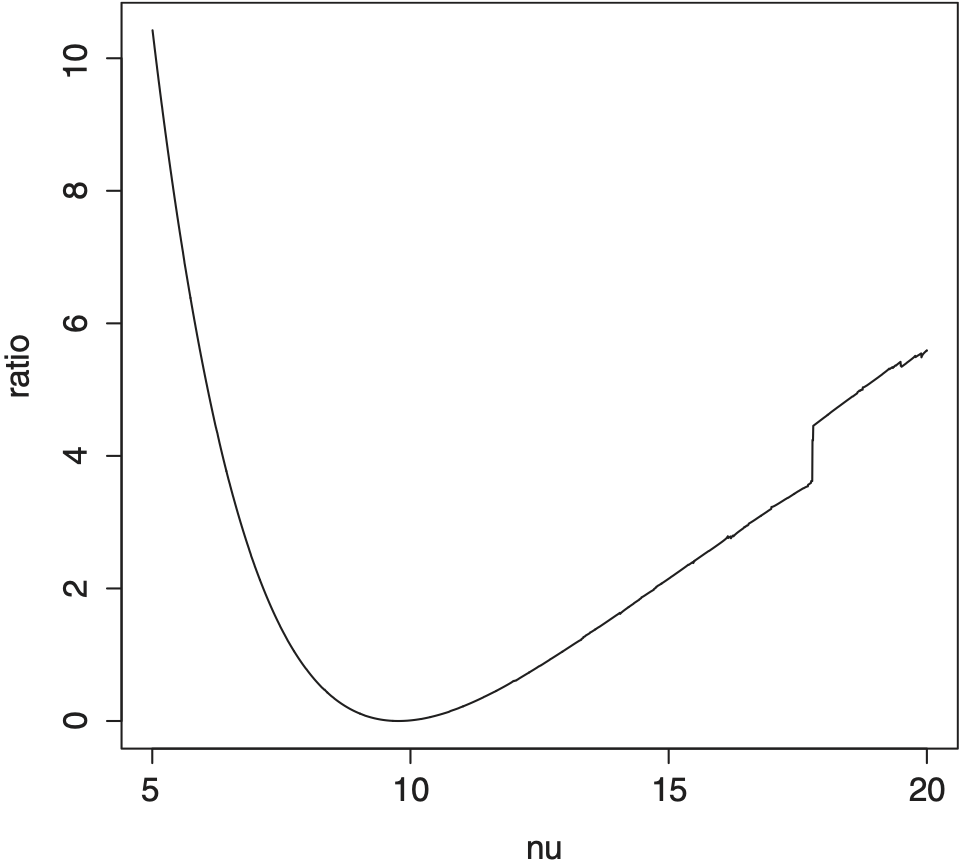
Finally, we fit the t copula to the nonzero losses to building and content in Danish fire insurance claims. This data set is available at www.ma.hw.ac.uk/~mcneil/, which comprises 2167 fire losses over the period 1980 to 1990. We find that ρ̂ = 0.134 and ν̂ = 9.474. The empirical likelihood ratio function l₁(ν) is plotted in Figure 3 against ν from 5.005 to 20 with step 0.005. The proposed jackknife empirical likelihood intervals for ν are (6.830,16.285) and (6.415,17.785) for levels 0.9 and 0.95 respectively, and the normal approximation based intervals for ν are (0.978,12.719) and (−2.242,13.070) for levels 0.9 and 0.95 respectively. The above negative value is due to some large values of the bootstrapped estimators of ν, which is a disadvantage of using the bootstrap method. It is clear that the proposed jackknife empirical likelihood intervals are shorter and more skewed to the right than the normal approximation based intervals.

Figure 3.The empirical likelihood ratio l₁(ν) is plotted against ν from 5.005 to 20 with step 0.005 for the nonzero losses to building and content in the Danish fire insurance claims

5. Proofs

Proof of Theorem 1. Define

\[ \begin{aligned} g(x, y) &=\operatorname{Esign}\left(\left(x-X_{1}\right)\left(y-Y_{1}\right)\right)-\tau \\ &=4\left\{C\left(F_{1}(x), F_{2}(y)\right)-\operatorname{E} C\left(F_{1}\left(X_{1}\right), F_{2}\left(Y_{1}\right)\right)\right\} \\ & \quad -2\left\{F_{1}(x)-\frac{1}{2}\right\}-2\left\{F_{2}(y)-\frac{1}{2}\right\}, \\ \psi\left(x_{1}, y_{1}, x_{2}, y_{2}\right) &= \operatorname{sign}\left(\left(x_{1}-x_{2}\right)\left(y_{1}-y_{2}\right)\right) \\ & \quad -g\left(x_{1}, y_{1}\right)-g\left(x_{2}, y_{2}\right) . \end{aligned} \]

It follows from the Hoeffding decomposition and results in Hoeffding (1948) that

\[ \begin{aligned} \sqrt{n}\{\hat{\tau}-\tau\}= & \frac{2}{\sqrt{n}} \sum_{i=1}^{n} g\left(X_{i}, Y_{i}\right) \\ & +\frac{2 \sqrt{n}}{n(n-1)} \sum_{1 s i j j s n} \psi\left(X_{i}, Y_{i}, X_{j}, Y_{j}\right) \\ = & \frac{2}{\sqrt{n}} \sum_{i=1}^{n} g\left(X_{i}, Y_{i}\right)+o_{p}(1), \end{aligned} \tag{5.1} \]

which implies Equation (2.1). By the Taylor expansion, we have

\[ \begin{aligned} 0 &= \frac{1}{\sqrt{n}} \sum_{i=1}^{n} l\left(\hat{\rho}, \hat{v} ; F_{n 1}\left(X_{i}\right), F_{n 2}\left(Y_{i}\right)\right) \\ & = \frac{1}{\sqrt{n}} \sum_{i=1}^{n} l\left(\rho, v ; F_{n 1}\left(X_{i}\right), F_{n 2}\left(Y_{i}\right)\right) \\ & \quad +\frac{1}{\sqrt{n}} \sum_{i=1}^{n}\left\{\frac{\partial}{\partial \rho} l\left(\rho, v ; F_{n 1}\left(X_{i}\right), F_{n 2}\left(Y_{i}\right)\right)\right\}(\hat{\rho}-\rho)\\ & \quad + \frac{1}{\sqrt{n}} \sum_{i=1}^{n}\left\{\frac{\partial}{\partial v} l\left(\rho, v ; F_{n 1}\left(X_{i}\right), F_{n 2}\left(Y_{i}\right)\right)\right\} (\hat{v}-v)+o_{p}(1) \\ & = \frac{1}{\sqrt{n}} \sum_{i=1}^{n} l\left(\rho, v ; F_{1}\left(X_{i}\right), F_{2}\left(Y_{i}\right)\right) \\ & \quad + \frac{1}{\sqrt{n}} \sum_{i=1}^{n} l_{u}\left(\rho, v ; F_{1}\left(X_{i}\right), F_{2}\left(Y_{i}\right)\right) \left\{F_{n 1}\left(X_{i}\right)-F_{1}\left(X_{i}\right)\right\} \\ & \quad + \frac{1}{\sqrt{n}} \sum_{i=1}^{n} l_{v}\left(\rho, v ; F_{1}\left(X_{i}\right), F_{2}\left(Y_{i}\right)\right)\left\{F_{n 2}\left(Y_{i}\right)-F_{2}\left(Y_{i}\right)\right\} \\ & \quad + \frac{1}{n} \sum_{i=1}^{n}\left\{\frac{\partial}{\partial \rho} l\left(\rho, v ; F_{1}\left(X_{i}\right), F_{2}\left(Y_{i}\right)\right)\right\} \sqrt{n}(\hat{\rho}-\rho) \\ & \quad + \frac{1}{n} \sum_{i=1}^{n}\left\{\frac{\partial}{\partial v} l\left(\rho, v ; F_{1}\left(X_{i}\right), F_{2}\left(Y_{i}\right)\right)\right\} \sqrt{n}(\hat{v}-v)+o_{p}(1), \end{aligned} \tag{5.2} \]

which implies Equation (2.2). More details can be found in Wang, Peng, and Yang (2013).

The values of σ²₁, σ₁₂ and σ²₂ can be calculated in a straightforward manner by using the Law of Large Numbers, which are given by

\[ \begin{array}{l} \sigma_{11}^{2}=\cos ^{2}\left(\frac{\pi \tau}{2}\right) \pi^{2}\left\{\begin{array}{l} 8 \int_{0}^{1} \int_{0}^{1}\left\{\begin{array}{l} 2 C^{2}(u, v) \\ -2(u+v) C(u, v)+u v \end{array}\right\} \\ d C(u, v)+\frac{5}{3}-\tau^{2}+2 \tau \end{array}\right\}, \\ \sigma_{2}^{2}=K_{v}^{-2}\binom{K^{2}+R_{1}+R_{2}+2 R_{3}+2 R_{4}+2 R_{5}+K_{\rho}^{2} \sigma_{1}^{2}}{+2 K_{\mathrm{\rho}}\left(L_{1}+L_{2}+L_{3}\right)}, \\ \sigma_{12}^{2}=-K_{v}^{-1}\left(K_{\rho} \sigma_{1}^{2}+L_{1}+L_{2}+L_{3}\right), \end{array} \]

where

\[ \begin{aligned} K^{2}= & \int_{0}^{1} \int_{0}^{1} l(\rho, v ; u, v)^{2} d C(u, v), \\ R_{1}= & \int_{0}^{1} \int_{0}^{1} \int_{0}^{1} \int_{0}^{1} l_{u}\left(\rho, v ; u_{1}, v_{1}\right) l_{u}\left(\rho, v ; u_{2}, v_{2}\right) \\ & \left(u_{1} \wedge u_{2}-u_{1} u_{2}\right) d C\left(u_{1}, v_{1}\right) d C\left(u_{2}, v_{2}\right), \end{aligned} \]

\[ \begin{aligned} R_{2}= & \int_{0}^{1} \int_{0}^{1} \int_{0}^{1} \int_{0}^{1} l_{v}\left(\rho, v ; u_{1}, v_{1}\right) l_{v}\left(\rho, v ; u_{2}, v_{2}\right) \\ & \left(v_{1} \wedge v_{2}-v_{1} v_{2}\right) d C\left(u_{1}, v_{1}\right) d C\left(u_{2}, v_{2}\right), \\ R_{3}= & \int_{0}^{1} \int_{0}^{1} \int_{0}^{1} \int_{0}^{1} l_{u}\left(\rho, v ; u_{1}, v_{1}\right) l_{v}\left(\rho, v ; u_{2}, v_{2}\right) \\ & \left(C\left(u_{1}, v_{2}\right)-u_{1} v_{2}\right) d C\left(u_{1}, v_{1}\right) d C\left(u_{2}, v_{2}\right), \\ R_{4}= & \int_{0}^{1} \int_{0}^{1} \int_{0}^{1} \int_{0}^{1} l_{u}\left(\rho, v ; u_{1}, v_{1}\right) l\left(\rho, v ; u_{2}, v_{2}\right) \\ & \left(I\left(u_{2} \leq u_{1}\right)-u_{1}\right) d C\left(u_{1}, v_{1}\right) d C\left(u_{2}, v_{2}\right), \\ R_{5}= & \int_{0}^{1} \int_{0}^{1} \int_{0}^{1} \int_{0}^{1} l_{v}\left(\rho, v ; u_{1}, v_{1}\right) l\left(\rho, v ; u_{2}, v_{2}\right) \\ & \left(I\left(v_{2} \leq v_{1}\right)-v_{1}\right) d C\left(u_{1}, v_{1}\right) d C\left(u_{2}, v_{2}\right), \\ L_{1}= & \cos \left(\frac{\pi \tau}{2}\right) \pi \int_{0}^{1} \int_{0}^{1} l(\rho, v ; u, v) \\ & \{4 C(u, v)-2 u-2 v\} d C(u, v), \\ L_{2}= & \cos \left(\frac{\pi \tau}{2}\right) \pi \int_{0}^{1} \int_{0}^{1} \int_{0}^{1} \int_{0}^{1} l_{u}\left(\rho, v ; u_{1}, v_{1}\right) \\ & \left\{4 C\left(u_{2}, v_{2}\right)-2 u_{2}-2 v_{2}\right\} \\ & \times\left\{I\left(u_{2} \leq u_{1}\right)-u_{1}\right\} d C\left(u_{1}, v_{1}\right) d C\left(u_{2}, v_{2}\right), \end{aligned} \]

and

\[ \begin{aligned} L_{3}= & \cos \left(\frac{\pi \tau}{2}\right) \pi \int_{0}^{1} \int_{0}^{1} \int_{0}^{1} \int_{0}^{1} l_{v}\left(\rho, v ; u_{1}, v_{1}\right) \\ & \left\{4 C\left(u_{2}, v_{2}\right)-2 u_{2}-2 v_{2}\right\} \\ & \times\left\{I\left(v_{2} \leq v_{1}\right)-v_{1}\right\} d C\left(u_{1}, v_{1}\right) d C\left(u_{2}, v_{2}\right) . \end{aligned} \]

Proof of Theorem 2. It follows from Equation (2.3) and the fact that

\[ \begin{aligned} \sqrt{n}(\hat{\lambda}-\lambda) & =\sqrt{n}(\lambda(\hat{\rho}, \hat{v})-\lambda(\rho, v)) \\ & =\sqrt{n} \frac{\partial \lambda}{\partial \rho}(\hat{\rho}-\rho)+\sqrt{n} \frac{\partial \lambda}{\partial v}(\hat{v}-v)+o_{p}(1) . \end{aligned} \]

Proof of Theorem 3. Here we use similar arguments in Wang, Peng, and Yang (2013). Write Z_i = Z_i(ν₀). Then it suffices to prove the following results:

\[ \frac{1}{\sqrt{n}} \sum_{i=1}^{n} Z_{i} \xrightarrow{d} N\left(0, \sigma_{3}^{2}\right) \text { as } n \rightarrow \infty, \tag{5.3} \]

\[ \frac{1}{n} \sum_{i=1}^{n} Z_{i}^{2} \xrightarrow{p} \sigma_{3}^{2} \text { as } n \rightarrow \infty, \tag{5.4} \]

and

\[ \max _{1 \leq i s n}\left|Z_{i}\right|=o_{p}(\sqrt{n}), \tag{5.5} \]

where σ²₃ = K²_ν σ²₂.

Write

\[ \begin{array}{l} \frac{1}{\sqrt{n}} \sum_{i=1}^{n} Z_{i}=\frac{1}{\sqrt{n}} \sum_{i=1}^{n} l\left(\hat{\rho}, v_{0} ; F_{n 1}\left(X_{j}\right), F_{n 2}\left(Y_{j}\right)\right) \\ \quad+\frac{1}{\sqrt{n}} \sum_{i=1}^{n} \sum_{j \times i}\left\{\begin{array}{l} l\left(\hat{\rho}, v_{0} ; F_{n 1}\left(X_{j}\right), F_{n 2}\left(Y_{j}\right)\right) \\ -l\left(\hat{\rho}_{i}, v_{0} ; F_{n 1, i}\left(X_{j}\right), F_{n 2, i}\left(Y_{j}\right)\right) \end{array}\right\} \end{array} \]

and using the arguments in the proof of Lemma 1 in Wang, Peng, and Yang (2013), we have

\[ \frac{1}{\sqrt{n}} \sum_{i=1}^{n} \sum_{j \neq i}\left\{\begin{array}{l} l\left(\hat{\rho}, v_{0} ; F_{n 1}\left(X_{j}\right), F_{n 2}\left(Y_{j}\right)\right) \\ -l\left(\hat{\rho}_{i}, v_{0} ; F_{n 1, i}\left(X_{j}\right), F_{n 2, i}\left(Y_{j}\right)\right) \end{array}\right\}=o_{p}(1) . \]

Hence, it follows from Equation (5.2) that

\[ \begin{aligned} \frac{1}{\sqrt{n}} \sum_{i=1}^{n} Z_{i}= & \frac{1}{\sqrt{n}} \sum_{i=1}^{n} l\left(\hat{\rho}, v_{0} ; F_{n 1}\left(X_{j}\right), F_{n 2}\left(Y_{j}\right)\right)+o_{p}(1) \\ = & \frac{1}{\sqrt{n}} \sum_{i=1}^{n} l\left(\rho, v_{0} ; F_{1}\left(X_{i}\right), F_{2}\left(Y_{i}\right)\right) \\ & +\frac{1}{\sqrt{n}} \sum_{i=1}^{n} l_{u}\left(\rho, v_{0} ; F_{1}\left(X_{i}\right), F_{2}\left(Y_{i}\right)\right) \\ & \left\{F_{n 1}\left(X_{i}\right)-F_{1}\left(X_{i}\right)\right\} \\ & +\frac{1}{\sqrt{n}} \sum_{i=1}^{n} l_{v}\left(\rho, v_{0} ; F_{1}\left(X_{i}\right), F_{2}\left(Y_{i}\right)\right) \\ & \left\{F_{n 2}\left(Y_{i}\right)-F_{2}\left(Y_{i}\right)\right\} \\ & +\frac{1}{n} \sum_{i=1}^{n}\left\{\frac{\partial}{\partial \rho} l\left(\rho, v_{0} ; F_{1}\left(X_{i}\right), F_{2}\left(Y_{i}\right)\right)\right\} \\ & \sqrt{n}(\hat{\rho}-\rho)+o_{p}(1) \\ = & -\frac{1}{n} \sum_{i=1}^{n}\left\{\frac{\partial}{\partial v} l\left(\rho, v_{0} ; F_{1}\left(X_{i}\right), F_{2}\left(Y_{i}\right)\right)\right\} \\ & \sqrt{n}\left(\hat{v}-v_{0}\right)+o_{p}(1) d \rightarrow N\left(0, \sigma_{3}\right), \end{aligned} \tag{5.6} \]

i.e., Equation (5.3) holds. Similarly we can show Equations (5.4) and (5.5).

Proof of Theorem 4. Write \(Y_i=n \hat{\rho}-(n-1) \hat{\rho}_i-\rho\). Similar to the proof of Theorem 3, it suffices to show that

\[ \frac{1}{\sqrt{n}} \sum_{i=1}^{n}\left(Z_{i}, Y_{i}\right)^{T} \xrightarrow{d} N(0, \Sigma) \text { as } n \rightarrow \infty, \tag{5.7} \]

\[ \frac{1}{n} \sum_{i=1}^{n}\left(Z_{i}, Y_{i}\right)^{T}\left(Z_{i}, Y_{i}\right) \xrightarrow{p} \Sigma \text { as } n \rightarrow \infty, \tag{5.8} \]

and

\[ \max _{1 \leq i \leq n}\left\|\left(Z_{i}, Y_{i}\right)^{T}\right\|=o_{p}(\sqrt{n}), \tag{5.9} \]

where

\[ \Sigma=\left(\begin{array}{ll} \sigma_{3}^{2} & K_{v} \sigma_{12} \\ K_{v} \sigma_{12} & \sigma_{1}^{2} \end{array}\right) . \]

Since \(\sum_{i=1}^{n}\left(\hat{\tau}-\hat{\tau}_{i}\right)=0 \text { and } \hat{\tau}-\hat{\tau}_{i}=O(1 / n)\) almost surely, we have

\[ \begin{array}{l} \frac{1}{\sqrt{n}} \sum_{i=1}^{n} Y_{i}=\sqrt{n}(\hat{\rho}-\rho)+\frac{n-1}{\sqrt{n}} \sum_{i=1}^{n}\left(\hat{\rho}-\hat{\rho}_{i}\right) \\ \quad=\sqrt{n}(\hat{\rho}-\rho)+\frac{n-1}{\sqrt{n}} \sum_{i=1}^{n}\binom{\frac{\pi}{2} \cos \left(\frac{\pi \hat{\tau}}{2}\right)\left(\hat{\tau}-\hat{\tau}_{i}\right)}{+O(1)\left(\hat{\tau}-\hat{\tau}_{i}\right)^{2}} \\ \quad=\sqrt{n}(\hat{\rho}-\rho)+O(\sqrt{n}) \sum_{i=1}^{n}\left(\hat{\tau}-\hat{\tau}_{i}\right)^{2} \\ \quad =\sqrt{n}(\hat{\rho}-\rho)+O(\sqrt{n}) \sum_{i=1}^{n}(O(1 / n))^{2} \\ \quad =\sqrt{n}(\hat{\rho}-\rho)+o_{p}(1) . \end{array} \]

Thus Equation (5.7) follows from Equations (2.3) and (5.6). Equations (5.8) and (5.9) can be shown by some similar expansions as in Wang, Peng, and Yang (2013).

Proof of Lemma 1. Similar to the proof of Theorem 3, we have

\[ \begin{array}{l} \frac{1}{\sqrt{n}} \sum_{i=1}^{n}\left\{\tilde{Z}_{i}\left(\nu_{0}\right)-\lambda_{0}\right\} \\ \quad=\left\{\frac{\partial \lambda}{\partial \rho}\left(\rho_{0}, \nu_{0}\right)\right\} \sqrt{n}\left(\hat{\rho}-\rho_{0}\right)+o_{p}(1) \end{array} \]

and

\[ \begin{array}{c} \frac{1}{\sqrt{n}} \sum_{i=1}^{n} Z_{i}\left(v_{0}\right)=-\frac{1}{n} \sum_{i=1}^{n} \frac{\partial}{\partial v} l\left(\rho_{0}, v_{0} ; F_{1}\left(X_{i}\right), F_{2}\left(Y_{i}\right)\right) \\ \sqrt{n}\left(\hat{v}-v_{0}\right)+o_{p}(1), \end{array} \]

where λ(ρ, ν) is defined in Theorem 2. That is, we can show that

\[ \frac{1}{\sqrt{n}} \sum_{i=1}^{n} Z_{i}^{*}\left(\nu_{0}, \lambda_{0}\right) \xrightarrow{d} N\left(0, \Sigma^{*}\right), \tag{5.10} \]

where the covariance matrix Σ* can be calculated by Equation (2.3). Further we can show that

\[ \frac{1}{n} \sum_{i=1}^{n} Z_{i}^{*}\left(\nu_{0}, \lambda_{0}\right) Z_{i}^{*^{T}}\left(\nu_{0}, \lambda_{0}\right) \xrightarrow{p} \Sigma^{*} \tag{5.11} \]

and

\[ \max _{1 \leq i \leq n}\left\|Z_{i}^{*}\left(v_{0}, \lambda_{0}\right)\right\|=o_{p}\left(n^{1 / 2}\right) \tag{5.12} \]

Hence, the lemma can be shown in the same way as Lemma 1 of Qin and Lawless (1994) by using Equations (5.10)–(5.12).

Proof of Theorem 5. Using the same arguments in the proof of Theorem 1 of Qin and Lawless (1994), it follows from Equations (5.10)–(5.12) that

\[ \binom{\tilde{\lambda}_{3}}{\tilde{v}-v_{0}}=S_{n}^{-1}\binom{-Q_{1 n}\left(v_{0}, 0\right)+o_{p}\left(n^{-1 / 2}\right)}{o_{p}\left(n^{-1 / 2}\right)}, \]

where

\[ \begin{aligned} S_{n} & =\left(\begin{array}{ll} \frac{\partial Q_{1 n}\left(v_{0}, 0\right)}{\partial \lambda_{3}} & \frac{\partial Q_{1 n}\left(v_{0}, 0\right)}{\partial v} \\ \frac{\partial Q_{2 n}\left(v_{0}, 0\right)}{\partial \lambda_{3}} & 0 \end{array}\right) \xrightarrow{p}\left(\begin{array}{cc} S_{11} & S_{12} \\ S_{21} & 0 \end{array}\right) \\ & =\left(\begin{array}{ll} -\mathrm{E}\left\{Z_{1}^{*}\left(v_{0}, \lambda_{0}\right) Z_{1}^{* T}\left(v_{0}, \lambda_{0}\right)\right\} & \mathrm{E}\left\{\frac{\partial Z_{1}^{*}\left(v_{0}, \lambda_{0}\right)}{\partial v}\right\} \\ \mathrm{E}\left\{\frac{\partial Z_{1}^{*}\left(v_{0}, \lambda_{0}\right)}{\partial v}\right\} T & 0 \end{array}\right) . \end{aligned} \]

By the standard arguments of the empirical likelihood method (see proof of Theorem 1 in Owen 1990), it follows from Lemma 1 that

\[ \begin{aligned} l_{3}( & \left.\tilde{\boldsymbol{v}}\left(\lambda_{0}\right), \lambda_{0}\right)=2 \sum_{i=1}^{n} \log \left\{1+\tilde{\lambda}_{3}^{T} Z_{i}^{*}\left(\tilde{\mathbf{v}}, \lambda_{0}\right)\right\} \\ & =2 n\left(\tilde{\lambda}_{3}^{T}, \tilde{\mathbf{v}}^{T}-\boldsymbol{v}_{0}^{T}\right)\left(Q_{1 n}^{T}\left(v_{0}, 0\right), 0\right)^{T} \\ & \quad +n\left(\tilde{\lambda}_{3}^{T}, \tilde{\mathbf{v}}^{T}-v_{0}^{T}\right) S_{n}\left(\tilde{\lambda}_{3}^{T}, \tilde{\mathbf{v}}^{T}-v_{0}^{T}\right)^{T}+o_{p}(1) \\ & =-n\left(Q_{1 n}^{T}\left(v_{0}, 0\right), 0\right) S_{n}^{-1}\left(Q_{1 n}^{T}\left(v_{0}, 0\right), 0\right)^{T}+o_{p}(1) \\ & =-\left(W^{T}, 0\right)\left(\begin{array}{ll} S_{11} & S_{12} \\ S_{21} & 0 \end{array}\right)^{-1}\left(W^{T}, 0\right)^{T}+o_{p}(1), \end{aligned} \tag{5.13} \]

as n → ∞, where W is a multivariate normal random variable with mean zero and covariance matrix S₁₁. Since

\[ \left(\begin{array}{ll} S_{11} & S_{12} \\ S_{21} & 0 \end{array}\right)^{-1}=\left(\begin{array}{ll} S_{11}^{-1}-S_{11}^{-1} S_{12} \Delta^{-1} S_{21} S_{11}^{-1} & S_{11}^{-1} S_{12} \Delta^{-1} \\ \Delta^{-1} S_{21} S_{11}^{-1} & -\Delta^{-1} \end{array}\right), \]

where Δ = S₂₁ S⁻¹₁₁ S₁₂, we have

\[ \begin{aligned} -( & \left(W^{T}, 0\right)\left(\begin{array}{ll} S_{11} & S_{12} \\ S_{21} & 0 \end{array}\right)^{-1}\left(W^{T}, 0\right)^{T} \\ = & -W^{T}\left\{S_{11}^{-1}-S_{11}^{-1} S_{12} \Delta^{-1} S_{21} S_{11}^{-1}\right\} W \\ = & \left\{\left(-S_{11}\right)^{-1 / 2} W\right\}^{T} S_{11}^{1 / 2}\left\{S_{11}^{-1}-S_{11}^{-1} S_{12} \Delta^{-1} S_{21} S_{11}^{-1}\right\} \\ & S_{11}^{1 / 2}\left\{\left(-S_{11}\right)^{-1 / 2} W\right\} \\ = & \left\{\left(-S_{11}\right)^{-1 / 2} W\right\}^{T}\left\{I-S_{11}^{-1 / 2} S_{12} \Delta^{-1} S_{21} 1_{11}^{-1 / 2}\right\} \\ & \left\{\left(-S_{11}\right)^{-1 / 2} W\right\} . \end{aligned} \tag{5.14} \]

Since

\[ \operatorname{tr}\left(S_{11}^{-1 / 2} S_{12} \Delta^{-1} S_{21} S_{11}^{-1 / 2}\right)=\operatorname{tr}\left(\Delta^{-1} S_{21} S_{11}^{-1} S_{12}\right)=1 \]

we have \(\operatorname{tr}\left(I-S_{11}^{-1 / 2} S_{12} \Delta^{-1} S_{21} S_{11}^{-1 / 2}\right)=1\) Hence it follows from Equations (5.13) and (5.14) that \(l_{3}\left(v\left(\lambda_{0}\right), \lambda_{0}\right) \xrightarrow{d} \chi^{2}(1)\) as n → ∞.

Acknowledgment

We thank the anonymous Variance reviewers for their helpful comments. Peng’s research was supported by the Actuarial Foundation.