Estimating Insurance Attrition Using Survival Analysis

1. Introduction

The retention ratio impacts both growth and profit, two important goals of insurance companies. Because of the importance of retention to insurance companies, CEOs often discuss it in earnings calls. Travelers commented in its 2010Q4 earnings call, “Given our strong retentions as well as the new business and account growth we’ve achieved over the last few years, we have significant positive leverage to an improving environment.” Allstate said in its 2010Q4 earnings call, “We were not successful in raising customer renewal rates, so that the new business success did not result in overall growth this quarter.”

In addition to profit and growth, effective marketing, underwriting, pricing, and customer service initiatives also depend on an accurate understanding of the retention/attrition of the customer. Gronroos (1994) points out that customer retention receives considerable attention in marketing research and practice. Reichheld and Sasser (1990) show that customer retention is a prime issue for firms to maximize profit and build a competitive advantage. Feldblum (1996) suggests that an insurance company should price risks to take into account the expected profitability over the lifetime of the policy, including the loss ratio, expense ratio, and retention level at each renewal. Ranaweera and Neely (2003) analyze the link between customer service and retention, and emphasize the importance of maintaining high retention through customer satisfaction and loyalty.

Insurance retention is often defined on an annual basis using snapshot data. For example, suppose a company had 1000 inforce policies at year-end 2009. If 900 of those 1000 policies were “in force” at year-end 2010, the retention is 90% (=900/1000). In this paper, retention is defined as the percentage of policies that are still effective after a year. Another popular definition of retention is the percentage of policies that are renewed at the expiration time. For example, if 100 policies were scheduled to expire in December 2010 and 95 policies were renewed, it is sometimes referred to as a 95% “retention” ratio. In this paper, we will refer to this second item as the renewal ratio. Renewal ratio is in general higher than retention ratio because a policy may leave its insurer after the renewal through a mid-term cancellation.

Conventional retention analysis focuses on whether or not the event of interest has occurred by some prespecified cutoff duration time. In insurance, the objective is often to estimate the likelihood that a policyholder will stay with the carrier for one year. Logistic or probit regressions are natural choices for modeling binary response variables. Sharma and Mahajan (1980), Lucas et al. (1987), and Peterson, Albaum, and Ridgway (1989) apply binary response models in marketing research on purchase decisions. Thomas, Edelman, and Crook (2002) show that logistic regression has become a standard method for credit risk analysis in the banking industry. The same assertion can probably be extended to insurance retention modeling. Despite the importance of retention to the insurance industry, there are few actuarial papers on retention analysis. However, there have been numerous presentations on insurance retention (Borgelt 2009; Tanser 2010, and Harbage 2010) at actuarial conferences. Because of the popularity of the generalized linear models (GLM) in insurance, insurance retention models are often presented under the GLM framework, as logistic (probit) regression can be thought of as a special case of GLM with binomial distribution and logit (probit) link function.

The binary retention models (such as logistic and probit regressions) have many advantages. First, they are easy to understand and explain. If a policy renews, the response variable in the regression is one; otherwise it is zero. Second, only snapshots of the inforce policies are needed for the binary retention analysis so that the data preparation is relatively simple. For example, year-end inforce policy data is readily available at almost all property and casualty insurance companies. Analysts can compare 2009 year-end inforce policies with 2010 year-end policies to determine whether a 2009 policy retained or left in 2010. Third, if the interest of the study is whether a policy will exceed the pre-specified duration time, binary models are powerful tools (Helsen and Schmittlein 1993).

The shortcomings of binary models are also well studied. By definition, binary models only analyze whether a customer will leave, but they do not tell when she will leave (Banasik, Crook, and Thomas 1999). If the topic of study is when, such as when a loan will default, logistic and probit regressions cannot help.

Many time-varying macroeconomic variables, such as unemployment rate, GDP change, and stock market return, may impact retention. Binary models cannot fully utilize the information from time-varying variables. Helsen and Schmittlein (1993) argue that, when time-varying variables are included in the model specification, the appropriate functional form will depend on the time path of the explanatory variables. Common ad hoc procedures, such as taking the within-horizon average values, fail to recognize the time-path differences of the predictor variables. Flinn and Heckman (1982) demonstrate that reliance on ad hoc procedures to cope with time-trended variables in logistic regression can produce pathological estimates.

Estimates from binary models do not allow the researchers to make predictions about either the expected duration time or the probability of the event happening to an individual policy for time intervals that are not integer multiples of the predefined horizon. For example, logistic regression based on year-end inforce datasets can only predict the likelihood of retention on a yearly basis. It cannot predict the probability that a policy will leave after 2.3 years.

In this paper, the authors propose to use survival analysis to model insurance retention and attrition. Survival analysis has been popular in biostatistics (Cnaan and Ryan 1989; Bull and Spiegelhalter 1997; Fleming and Lin 2000) and is becoming popular in the banking industry (Stepanova and Thomas 2002; Andreeva 2006; Tang et al. 2007). Compared with conventional binary models, survival analysis has the following advantages. First, the response variable in survival analysis is the continuous time, not yes or no. For example, if Policy A stays with an insurer for 2.75 years (cancels the third term at the 9th month), the response variables for the three policy terms are 12, 24, and 33. In logistic regression, the responses would be 0, 0, and 1. Because the response variable is time, the model predicts when a policy will leave, not just whether a policy will leave.

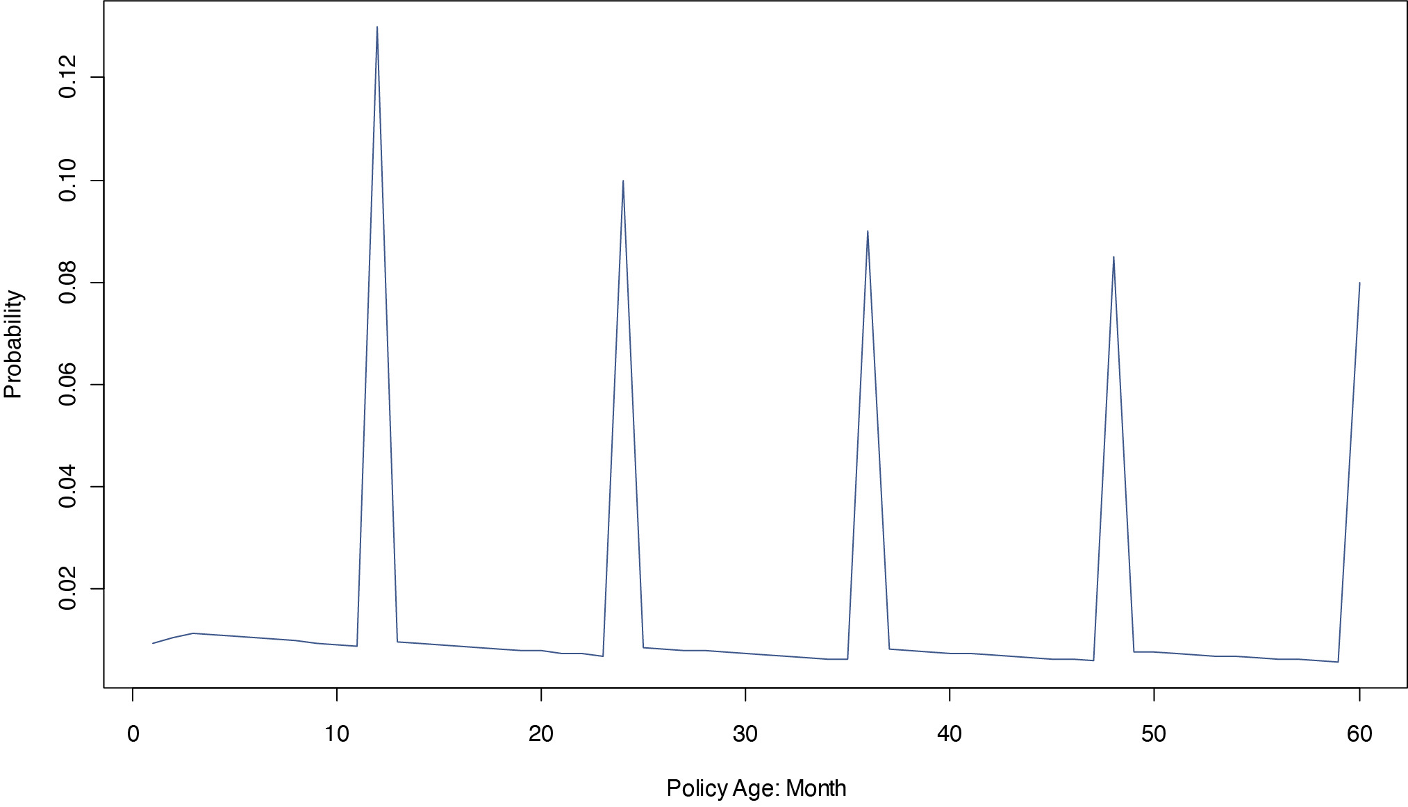
Second, insurance attrition comes from end-term nonrenewal and mid-term cancellation. Conventional binary models from snapshot data don’t differentiate between nonrenewal and cancellation.^[1] Using the example above, suppose another Policy B does not renew at the end of the third term. In binary models, the response variables for Policies A and B are the same. In survival analysis, the researcher differentiates Policy A from B, and treats A and B as a mid-term cancellation and a nonrenewal, respectively. The two sources of attrition result in a strong pattern of seasonality. When a new annual policy becomes effective, the likelihood of monthly attrition through cancellation in the middle of the term is relatively small. In the last month of the term, the probability of attrition through nonrenewal jumps significantly. If the policy renews, the probability of attrition will remain low for 11 months until it reaches the 2nd renewal at the 24th month. This cycle of seasonality continues into later terms. Figure 1 illustrates the monthly pattern of insurance attrition. If a new business (NB) policy originates in March and cancels in October of the same year, it will not be present in the year-end snapshot data. The information from those mid-term cancellation NB policies would be missing in logistic regression. Survival analysis is a panel data approach. It connects multiple policy terms from the same account and models them sequentially. Logistic regression, by contrast, treats individual terms from the same policy as independent records.^[2] By examining policy terms sequentially, survival analysis is able to utilize more information and provide a dynamic view of policy retention and attrition.

Figure 1.Probability of attrition: cancellation vs. nonrenewal

Third, survival analysis can take advantage of time-varying macroeconomic data. General economic conditions affect insurance retention. For example, unemployment rate increases may reduce retention and exposures. Many insurance companies experienced retention reductions during the great recession, especially in the contractor segment of business insurance. GDP growth may increase the probability of retention. These macroeconomic variables are not constant and can vary significantly within a policy term. In the framework of binary models using snapshot data, researchers can only use one summarized value over a time horizon for a macroeconomic variable. Helsen and Schmittlein (1993) point out that the duration time to the event of interest depends on the path of the predictive variables. Using one value instead of a series of values can produce significant estimation bias.

Survival analysis also has its disadvantages. First, the outputs of survival analysis cannot be applied as straightforwardly as those from binary models. Using logistic regression, the likelihood of retention after one year is a direct output of the model. Using survival analysis, one has to calculate the baseline survival function for the next several months, and then derive the survival function of each policy to calculate the expected annual retention ratio. This is a drawback of analyzing and predicting cancellation and nonrenewal sequentially. Second, although survival analysis can help actuaries to understand the relationship between retention and time-varying macroeconomic variables, it is difficult to capitalize on this knowledge in the real-world implementation because those macroeconomic variables are often more difficult to predict than the retention itself. Banks usually have professional teams to forecast major macroeconomic variables such as unemployment and interest rates. Most property and casualty insurance companies may not have this capacity.

This paper is organized in a straightforward manner. Section 2 introduces the theory of survival analysis, with particular focus on the proportional hazard model. Section 3 discusses how to prepare the panel data for survival analysis, while noting the data differences between survival model and logistic regression. Section 4 will provide a case study using survival analysis. The results from the proportional hazard model will be compared with those from logistic regression. The validation from holdout sample data demonstrates the theoretical advantages of survival analysis over the conventional logistic regression. Section 5 offers a summary of the main conclusions drawn from this analysis.

2. Survival analysis and the proportional hazard model

2.1. Survival analysis

Survival analysis is also named as time to event analysis or duration analysis. Kaplan and Meier (1958) pioneered the study of survival analysis and proposed to estimate survival functions from lifetime data using a series of horizontal steps of declining magnitude. Cox (1972) introduced the proportional hazard model, which examines the statistical relationships between a set of covariates and the survival function without assuming potentially questionable hazard distributions. Cox’s proportional hazard model represents a milestone, as it significantly improves the applicability of survival analysis.

Survival analysis was used predominantly in biomedical sciences where the dependent variable of study is often time to death (Oakes 2001). It is being widely applied in social and economic sciences when the research objective is to examine the time to a specific event such as unemployment (Arrow 1996), divorce (Hartley et al. 2010), product purchase (Helsen and Schmittlein 1993), loss of customer (Van den Poel and Lariviere 2004), or loan defaulting (Stepanova and Thomas 2002). In this paper we focus on insurance retention and attrition. The event of interest is the policy attrition (either through end-term nonrenewal or mid-term cancellation).

The most important concepts in survival analysis are survival and hazard functions. Let T denote the time until attrition occurs. The survival function, S(t), is defined as

$$S(t)=\operatorname{Prob}\{T \geq t\}, \quad \text { where } t \geq 0 \text {. }$$

The survival function is the probability that the attrition occurs later than some specified time t. The lifetime distribution function, F(t), is the complement of the survival function: F(t) = 1 − S(t). The derivative of F(t), $f(t)=\frac{d F(t)}{d t} \text {, }$ is the density function or event density. The density dt function represents the rate of attrition per unit of time. The hazard function, h(t), is the ratio of the density function to the survival function, $h(t)=\frac{f(t)}{S(t)}$ The hazard function is a measure of the tendency of attrition: the greater the value of the hazard function, the greater the probability of attrition. In actuarial science, the hazard function is often called the force of mortality.

The most popular survival distributions are the exponential and Weibull. The survival and density functions associated with the exponential distribution are $S(t)=e^{-\lambda t}$ and $f(t)=\lambda e^{-\lambda t}$, respectively. The hazard function for the exponential distribution is constant, $h(t)=\lambda$. The survival and density functions associated with the Weibull distribution are $S(t)=e^{-\beta t^\alpha \alpha}$ and $f(t)=\alpha \beta t^{\alpha-1} e^{-\beta t^\alpha}$, respectively. The hazard function of the Weibull distribution is $h(t)=\alpha \beta t^{\alpha-1}$. When $\alpha>1$, the hazard rate is increasing with time. When $\alpha<1$, hazard rate is decreasing.

Time to event in real applications is often not known because the event of interest may not occur prior to the end of study. This is called “right censoring.” In the context of insurance attrition analysis, if a policy is still effective with an insurance company when the study ends, the data is right-censored. We know the policy will eventually leave, but we do not know when it will leave. Right censoring implies that the duration time is only partially known (above a certain value). Survival analysis provides a powerful tool to utilize this partial information without introducing statistical bias (Lagakos 1979).

2.2. Proportional hazard model

Cox (1972) introduced the proportional hazards model to assess the effect of multiple covariates (explanatory variables) on survival time. The Cox model makes no assumptions on the nature or shape of the hazard function. Instead, it assumes that the underlying hazard rate (rather than survival time) is a function of the independent variables. The model can also take advantage of time-dependent covariates. These desirable features make Cox’s proportional hazard model the most popular approach in survival analysis.^[3]

The Cox’s proportional hazard model equation can be written as

$$h\left(t \mid x_{t}\right)=h_{0}(t) e^{\beta x_{t}} \tag{2.1}$$

where h(t|x_t) denotes the hazard rate at time t for an individual having covariate value x_t, where x_t = $\left(x_{1 t}, x_{2 t}, \ldots, x_{k t}\right)$; and $\beta=\left(\beta_1, \beta_2, \ldots, \beta_k\right)$, where k is the total number of the covariates, and $\beta_j$ is the constant proportional effect of x_j. The term $h_0(t)$ is called the baseline hazard; it is the hazard for the respective individual when there are no covariate impacts. The exponential term $e^{\beta^{\prime} x_t}$ is the parameter component, describing how the hazard varies in response to explanatory covariates. Dividing both sides of Equation (2.1) by $h_0(t)$ and then taking the natural logarithm of both sides, we can obtain a linear transformation of the model:

$$\log \left\{h\left(t \mid x_{t}\right) / h_{0}(t)\right\}=\beta x_{t} \tag{2.2}$$

The statistical estimation of β has been studied extensively. One of the popular numerical solutions is the semi-parametric partial maximum likelihood method by Helsen and Schmittlein (1993).

Like other concepts in survival analysis, the partial likelihood function is also related to time. Suppose that individual policy i leaves the insurer at duration time t. At t, a number of other policies were “at risk,” or effective with the company. Of all those at risk, policy i is the one that actually experienced the event (attrition) at t. The partial likelihood that this duration t indeed happened to policy i (and not to one of the other policies at risk) is

$$L\left(i \mid t, R_{t}\right)=\frac{h_{i}(t)}{\sum_{j \in R_{t}} h_{j}(t)}=\frac{\exp \left(\beta x_{i, t}\right)}{\sum_{j \in R_{t}} \exp \left(\beta x_{j, t}\right)} \tag{2.3}$$

where R_t represents the risk set at t (the group of policies that are still effective immediately before t). The partial likelihood estimate of $\beta$ can be obtained by maximizing the product of expression (2.3) over all observed duration times.

3. Survival analysis data construction

To create survival analysis data for insurance attrition, it is important to understand the difference between calendar time and duration time in the study. The concept of duration time is reflected in Figure 2, where the vertical line “|” represents the original inception date of the policies and each black triangle reflects the entry time in the study. The exhibit below shows four policies (A, B, C, and D) with varying inception times. Two policies (B and D) were still effective when the study ended and so are shown with simple circles at the end of the study to indicate that these policies were censored. The policies A and C ended with black squares experienced attrition. Thus, in calendar time both the entry and the exit time of the policies are staggered and can occur at any time throughout the course of the study. Duration time implies the length of time that the policies were a part of the study. Thus, every policy starts at time zero and has an ending point either when it experienced attrition or reached the end of the study (censored).

Figure 2.Calendar time vs. duration time in survival analysis

Table 1 provides more detailed information on the data construction using the example in Figure 2. Suppose the horizon of study is between 01/01/2000 to 12/31/2003. To create survival data, we only keep the policies for which the effective dates are within this predefined period of time. Policies A and B originate after the study starts, while C and D originate before the start date. The original inception dates are 01/01/2001, 07/01/2001, 03/01/1998, and 01/01/1997 for policies A through D, respectively. Policy A did not renew for the third term and ended its tenure at 12/31/2002. Policy C canceled the term at 11/30/2001. Policies B and D were inforce at the 12/31/2003, the end of study. The entry date of a policy is the effective date of the policy term immediately following the start time of study, as shown in Figure 2. For policies A and B, the entry dates are equal to the origination dates. For policy C, the entry time is 03/01/2000, two years after the origination. For Policy D, the entry time is three years after the origination. The start month (T1) of a specific policy term is defined as the number of months between the entry time and the start point of the term. The end month (T2) is the difference between the entry time and the end point of the policy term, which can be term expiration time, attrition time, or the end of study. Using policy C as an example, the entry time is 03/01/2000. The end time of the policy is 11/30/2001 when it canceled in its fourth term. The end month of the third record for Policy C is 21 months (11/30/2001 minus 03/01/2000). Policy C enters the study at its third term (the first two terms are out of the study horizon) and the time from the entry to the end of the third term is 12 months (03/1/2000–02/28/2001). Thus the end month for the survival analysis is 12 for the first record of Policy C. From the entry point to the end point of the fourth term is 21 months. So the end month is 21 for the second record of policy C. Policies B and D are still active at the end of the study so that the right-censor indicators are one for these two policies.

We now illustrate the estimation of partial likelihood, assuming that there are only four policies in the study. Policy A leaves the insurer at the 24th month. At t = 24, three policies (A, B, and D) are “at risk,” while policy C has already left. So the partial likelihood of policy A leaving at the 24th month is

$$L\left(A \mid 24, R_{24}\right)=\frac{\exp \left(\beta x_{A, 24}\right)}{\exp \left(\beta x_{A, 24}\right)+\exp \left(\beta x_{B, 24}\right)+\exp \left(\beta x_{D, 24}\right)} \tag{3.1}$$

All the explanatory variables at the 24th month are available in the data (Table 1).

Policy B is “at risk” of cancelling its insurance at the 30th month. At t = 30, policies A and C already left. Two policies (B and D) are in the risk set R₃₀. So, the partial likelihood of policy B’s attrition immediately after the 30th month is

$$L\left(B \mid 30, R_{30}\right)=\frac{\exp \left(\beta x_{B, 30}\right)}{\exp \left(\beta x_{B, 30}\right)+\exp \left(\beta x_{D, 30}\right)} \tag{3.2}$$

To calculate the partial likelihood in Equation (3.2), we need all the explanatory variables for policies B and D at t = 30, $x_{B, 30}$ and $x_{D, 30}$. The variables $x_{B, 30}$ are readily available in Table 1 because policy B is at the end of study time at the 30th month. The variables $x_{D, 30}$ are not readily available as there is no transaction record for policy D at the 30th month. In this case, to simplify the calculation, we obtain the values of those variables from the records immediately before the 30th month. So $x_{D, 24}$ would be used to replace $x$ in Equation (3.2) to calculate the partial likelihood function.^[4]

4. Case study

4.1. Data

To illustrate the survival analysis, we conduct a case study using simulated data from a commercial line book consisting of small business policies. The policy term is one year. A proportional hazard model is applied to six and half years of data containing over a million policy terms. Table 2 summarizes the traditional retention analysis by comparing the inforce policies at year ends 1 and 4. By row 1 of Table 2, there were a total of 197,954 inforce policies at the end of year 0. 156,477 policies were still effective at the end of year 1. The retention ratio is 79.05%. The total number of attritions during year 1 is 41,477. Among those attritions, 24,570 policies did not renew at the end of their terms and 16,907 policies canceled in the middle of their terms. The non-renewal and mid-term cancellation ratios are 12.41% and 8.54%, respectively. Most P&C actuaries are familiar with the retention measure in Table 2. Table 3 shows a monthly view of retention, and provides more detailed information that may not be included in standard reports of retention. By row 1 of Table 3, there were 199,099 inforce policies at the end of February of year 1. Among those policies, 16,938 policies would expire in March and 182,161 policies would expire in other months. During March, 87.68% of 16,938 policies (or 14,852) renewed, while 12.32% or 2,086 policies did not renew. Among those 182,161 policies with non-March expiration months, 0.88% or 1,609 policies canceled their terms during March; 99.12% or 180,552 policies remained effective. The mid-term cancellation percentages in Table 2 are much larger than those in Table 3 because the former is based on the number of cancellations in a full year while the latter is the same measure but within a month.

To create the panel data for survival analysis, we follow the general steps outlined in section 3. Internal data such as premium, loss, billing, and payments are at transaction level. External data, such as financial and macroeconomic variables, are month-end snapshot information. Many explanatory variables are constructed, including internal policy information (price change, policy age, policy size, risk types, limits, industry, package indicator, prior claims, late payments, payment frequency, etc.), external financial and credit information (age of business, number of inquiries, number of lawsuits, ownership indicator, commercial credit score, etc.), and macroeconomic information (GDP changes, stock index changes, inflations, interest rates, unemployment rates, market cycle, etc.).

Premium increase is often a top cause of attrition. Because of the importance of understanding the sensitivity of retention to price changes, retention models are often called “price elasticity models” in the context of price optimization projects. “Price change” is not as simple as comparing the premiums of adjacent terms because premium changes may be from non-rating reasons, such as changes from exposures (adding a vehicle, reducing payroll), coverages (increasing limit, removing an endorsement), and risk characteristics (having a claim, improving financial stability). To examine the attrition sensitivity to price change, we removed the premium impacts of non-rating factors to obtain the pure “price change.”

If a policy is active at the end of the study, the right-censor indicator is one for every record of the policy. If a policy is canceled in the middle of a term or not renewed at the end of a term, the right-censor indictor is zero for all its policy terms. When a record has zero earned premium, the record is deleted. If the duration of the last record within a policy panel is an integer multiple of a full policy term and the right-censor indictor is zero, the record is an end-term nonrenewal. If the duration of the last record is not a multiple of policy term and the right-censor indictor is zero, the record is a mid-term cancellation. By this rule, flat cancellation (an insurer books a premium when the renewal notice is sent out, and later offsets all the premium after the policyholder decides not to renew) is treated as end-term nonrenewal. In the whole modeling dataset, 830,874 records are right censored, 573,223 records are not censored. Among those 573,223 termination records, 307,454 are end-term nonrenewals and 265,769 are mid-term cancellations.

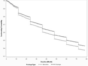
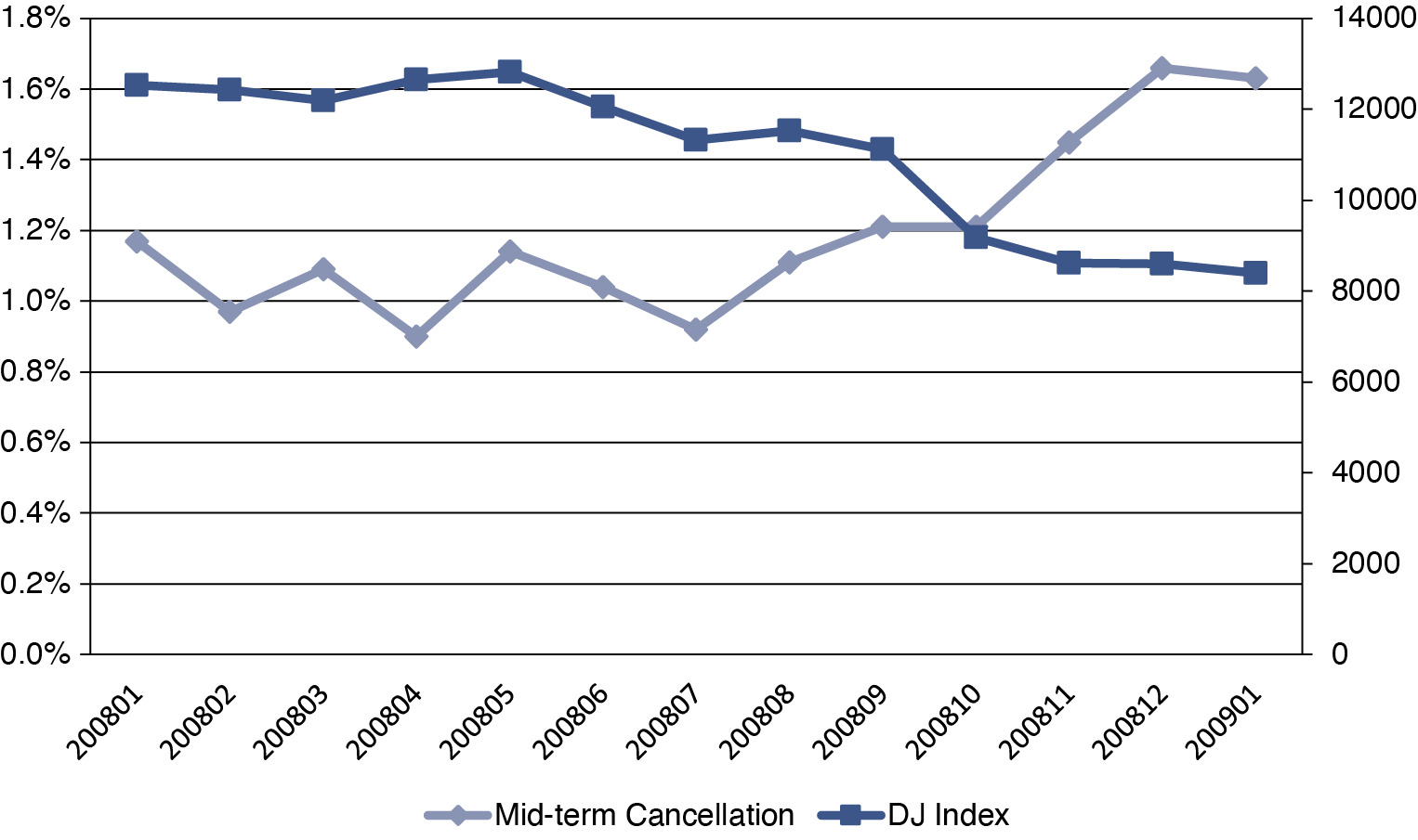
To detect the retention and attrition patterns by individual variables, we check the annual and monthly retention and attrition tables for numerous variables.^[5] It is well known that new business has lower retention than renewal business (Wu and Lin 2009). Tables 4 and 5 exhibit the annual retentions for new business and renewal business, respectively. Package policies generally have better retentions than mono-line policies.^[6] Tables 6 and 7 show the retentions for package and mono-line policies, respectively. Tables 4 to 7 confirm that renewal business and package policies are more likely to renew at the end of term and less likely to cancel in the middle of the term compared with their counterparts. Figure 3 illustrates how contractors’ mid-term cancellation moved with the Dow-Jones index in 2008. No single value can reflect what happened in the stock market in the year: the index was relatively flat in the beginning of the year with low volatility, yet it crashed in the second half of the year after the Lehman Brothers bankruptcy. The mid-term cancellation ratio in small contracting risks displays a similar pattern: it was relatively flat in the first half of the year. As the economic condition worsened in the 2nd half of the year, more contractors were out of business and no longer needed insurance. As a result, the attrition ratio through mid-term cancellations jumped up significantly. Using survival analysis, the authors are able to model how this specific path of the Dow-Jones index affects monthly (or even weekly) retention and attrition.

Figure 3.Dow Jones Index vs. small contractor mid-term cancellation ratio in 2008

4.2. Regression results

Proportional hazard model and logistic regression are developed using the data from year 0 to year 5. To create the data for logistic regression, year-end snapshot datasets are joined and stacked. For example, we left join year 0 data with year 1 data. If a policy was effective at the end of year 1, the attrition is 0, otherwise it is 1. Repeating this step using the data of later years and stacking five annual datasets together, we obtain the data for logistic regression. Because year-end snapshot data is used to construct the data for logistic regression, we do not know whether an attrition is due to end-term nonrenewal or mid-term cancelation. For time-varying macroeconomic variables, 12-month straight averages are used in the logistic regression. Table 8 reports the coefficients of four selected variables from survival analysis: “price change,” package indicator, policy age, and GDP change. Table 9 displays the coefficients of those variables from logistic regression.

Both survival analysis and the logistic model provide coefficients that are consistent with business knowledge. The sign of the coefficient for “price change” is positive. So rate increases will drive up the probability of attrition. The signs of coefficients for policy age and package indicator are negative, implying that older and package policies are more likely to stay with an insurer. GDP growth represents a broad economic environment. The negative coefficients of GDP growth imply that the retention ratio is higher in a better economy.

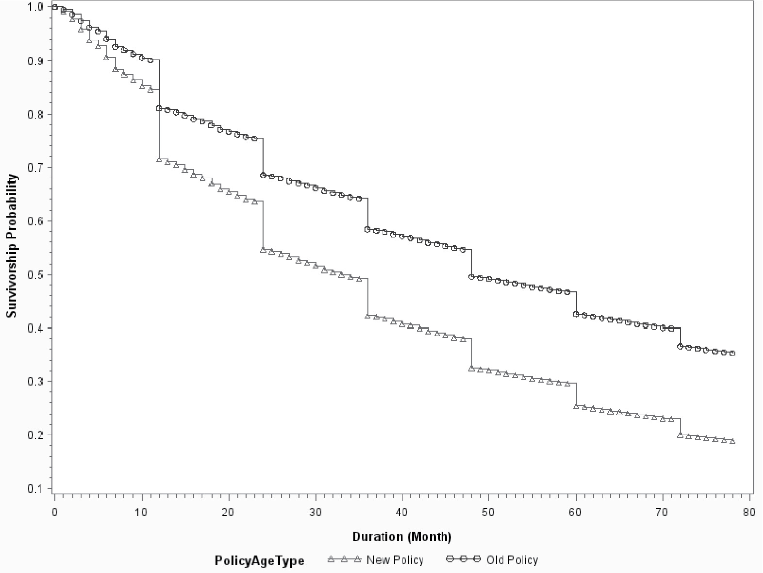
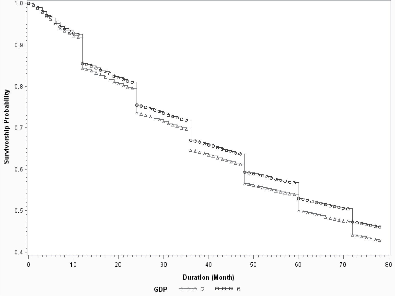
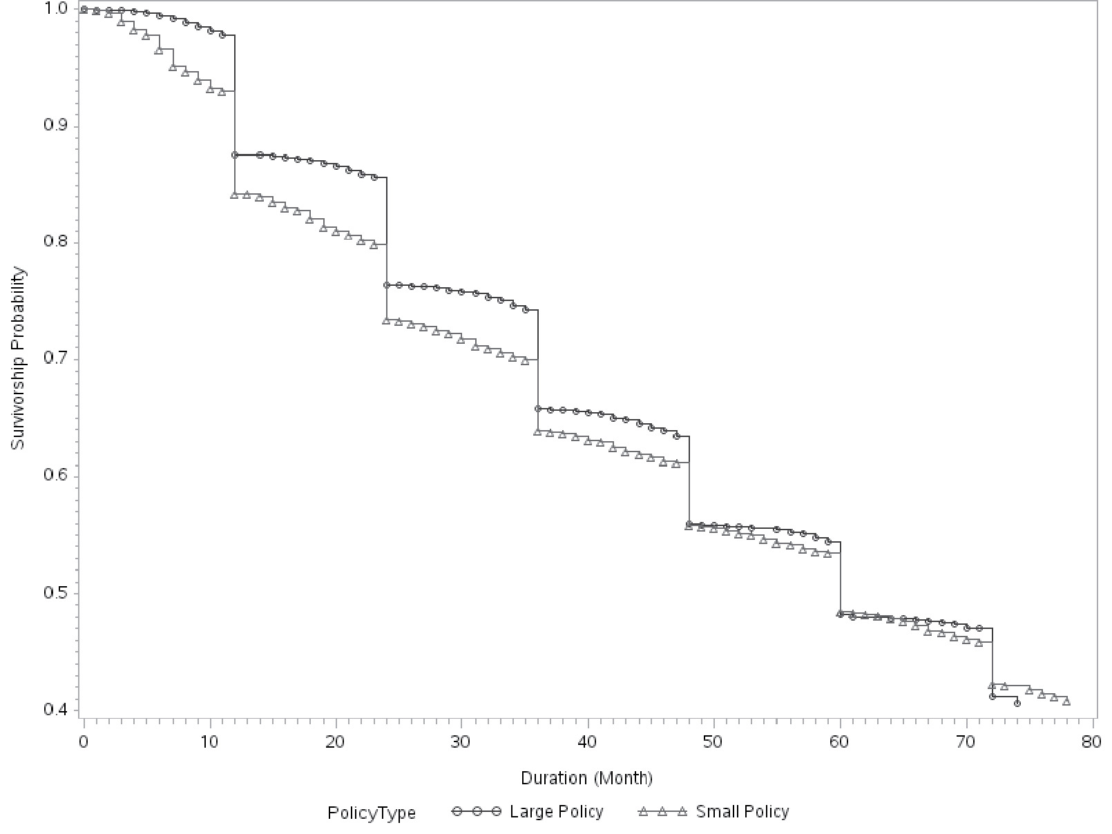
Figures 4 to 6 show the baseline survival curves of new business vs. 5-year old policies, package vs. monoline, and 2% GDP growth vs. 6% growth, respectively. The cumulative survival probabilities are derived assuming other variables are at their average values. In Figures 4 and 5, the blue lines are above the red lines, which demonstrates that old/package policies are more likely to renew than are young/mono-line policies. Figure 6 illustrates that policyholders have higher retention ratios in a good economy than in a bad economy. The advantages of survival analysis can also be illustrated by the survival curves in those figures. Logistic regression provides the likelihood of retention on a yearly basis. However, it cannot make predictions about either the expected duration time or the probability of attrition for time intervals that are not integer multiples of the predefined horizon. On the contrary, the survival curve offers predictions on a monthly basis as shown in Figures 4 to 6. This allows the survival model to investigate not only “whether” but also “when” a policy will leave. Figure 7 demonstrates this advantage by comparing the survival curves of two individual policies, a large policy vs. a small policy. The two policies have almost identical survival rates at the end of the fifth year. However, the survival curves of two policies are very different at various points of time. The small policy has much higher mid-term attrition ratios because small business owners are more likely to become bankrupt, sell the business, or change location, and all those activities can result in mid-term cancellations. Large polices have more negotiation powers and are more likely to switch insurance carriers if they do not get favorable renewal prices or desirable coverages. Insurance agencies are also more willing to quote with multiple carriers for a large client upon its renewal to keep the account. So, large policies tend to have higher end-term nonrenewal ratios. Logistic regression can predict the annual attrition probability, but cannot tell the month-by-month attrition differences through mid-term cancellation or end-term nonrenewal. In practice, understanding “when” or the timing difference of attrition is important. End-term nonrenewal is more sensitive to the renewal price change and therefore is more controllable by an insurance company, as it can adjust the pricing strategy to manage the retention. Attrition in the non-expiration months is more difficult to manage. Certain types of mid-term cancellations are even unmanageable. For example, bankruptcies and ownership changes are beyond the control of the insurance company.

Figure 4.Survival curves for new vs. 5-year policies

Figure 5.Survival curves for package vs. monoline policies

Figure 6.Survival curves by GDP growth: 2% vs. 6%

Figure 7.Survival curves by policy size: large vs. small

4.3. Model validation

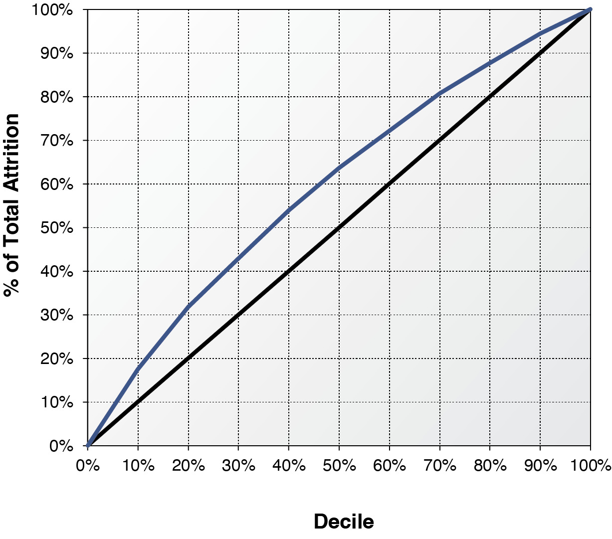
To validate the results from survival analysis and logistic regression, we randomly split the data into a development dataset and a validation dataset. The data for survival analysis is slightly larger than that of logistic regression because some partial-term policies are in the survival analysis, but not in the logistic regression. To conduct a fair model validation, we exclude from survival analysis those policies that are not in logistics data from both development and validation datasets. Survival analysis predicts attrition on a monthly basis while logistic regression predicts attrition on an annual basis. We roll up the monthly predictions based on the monthly baseline of survival function from survival analysis to derive the probability of annual attrition. Model parameters of both survival analysis and logistic regression are derived from the same development data. Those parameters are used to score the policies in the same validation data. It is difficult to predict the macroeconomic variables when applying survival analysis to estimate future attrition. To deal with this practical concern, we used the values of macroeconomic variables at the month immediately before the policy effective month to score the policies in the validation data. Those out-of-sample policies are then ranked by decile using both survival scores and logistic scores from high to low. Decile one implies the highest predicted probability of annual attrition while decile ten implies the lowest probability. Tables 10 and 11 report the actual out-of-sample annual attrition ratios by decile for the survival analysis and the logistic regression, respectively. By comparing the attrition rates, survival analysis produces a lift marginally better than the logistic regression. The decile-one attrition ratios from the survival analysis and logistic regression are 38.41% and 37.07%, respectively. Survival analysis marginally outperforms the logistic regression by 1.3% in identifying the policies that are most likely to leave. The decile-ten attrition ratios from the survival analysis and logistic regression are 10.95% and 11.62%, respectively. Survival analysis and logistic regression are almost the same in identifying the policies that are most likely to stay, though survival analysis performs slightly better. Figures 8 and 9 demonstrate the lifts of the two methods graphically. The horizontal axis represents the model deciles and the vertical axis represents the accumulative percentage of attrition counts by decile. If a model cannot predict the probability of attrition at all, the lift will be a straight 45-degree line. The area of the lift curve above the diagonal line multiplied by two is often called the Gini coefficient, which is one of most popular measures of lift. A greater value of the Gini coefficient implies a stronger predictive performance. The Gini coefficient of the survival analysis is 0.199, marginally higher than 0.192, the Gini coefficient of logistic regression. The out-of-sample validation result is consistent but less significant compared with that from Helsen and Schmittlein (1993). The lift from survival analysis is only marginal better because (1) some partial-term policies, which have high predicted attrition probabilities from survival analysis, are excluded in measuring the lift, and (2) the theoretical advantage of using time-varying macroeconomic variables cannot be materialized in practice. The survival analysis can contemplate the macroeconomic dynamics in Figure 3. But very few economists could predict the exact path of Dow Jones index in 2008. Using a series of predicted values to project the attrition ratios may introduce more projection biases and parameter uncertainties. Survival analysis is powerful in helping actuaries to understand the relationship between macroeconomic variables and insurance attritions. This advantage provides great explanatory value but little predictive value.^[7] If we include the partial term policies and use actual month-by-month values of macroeconomic variables to score the attrition probability, the out-of-sample lift from survival analysis will become significantly stronger at 0.238. The stronger performance of survival analysis is expected because of the methodological advantages outlined in the paper.

Figure 8.Lift curve: survival analysis

Figure 9.Lift curve: logistic regression

5. Conclusions

Retention impacts both the bottom line and top line of insurance companies. Higher retention implies higher sales volumes, assuming a constant amount of new business. This improves the size of sales or the top line of an insurance company. Higher retention implies that a greater percentage of business is from more profitable renewal policies. This improves the profit or the bottom line.

In addition to profit and growth, retention is a crucial factor in many marketing, underwriting, pricing, and customer service initiatives. For example, the lifetime value of a customer cannot be accurately estimated without an accurate understanding of the retention tendency of the customer. To develop a pricing strategy that optimizes profits (or maximize sales under a certain profit constraint), one first has to understand the sensitivity of retentions under various pricing scenarios.

In this paper, the authors apply survival analysis as an alternative approach to the dominant binary regressions to analyze insurance attrition. Binary models use discrete yes and no as the response variable and can be used to answer the question of whether a policy will leave. Survival analysis uses the continuous time as the response variable and can be used to answer not only whether but also when a policy will leave. Conventional binary models are usually developed from snapshot data. Snapshot data does not contain the information on whether attrition is due to end-term nonrenewal or mid-term cancellation. Insurance attrition follows a strong seasonality: in the expiration month, a significant number of policies do not renew; while in other months, the attrition through mid-term cancellation is much smaller. Survival analysis is able to model the cancellation and nonrenewal sequentially and capture this seasonality of attrition well. In practice it is important for insurance companies to understand the attrition probabilities at various points of time. End-term nonrenewal is more sensitive to renewal prices and an insurance company can effectively manage this type of attrition through its pricing strategy. Mid-term cancellation can be from events that are out of an insurer’s control, such as bankruptcy, ownership change, or location change. Many time-varying macroeconomic variables affect insurance retention and attrition. Survival analysis can take into account the time path of those macroeconomic variables, and measure the impact of broad economic environment on retention accurately. A case study on a commercial line small-business book is performed to illustrate the survival analysis approach and to demonstrate its advantages. Survival analysis serves as an alternative to the dominant approach of binary regressions and supplements actuaries’ toolkit. It may help actuaries to improve their understanding of retention in terms of the macroeconomic environment (unemployment, GDP, interest rate, market cycle), the company’s pricing decisions (base rate change, multi-policy discount), and individual policies’ characteristics (age, policy tenure, credit).