Incorporating Spatial Dependence and Climate Change Trends for Measuring Long-Term Temperature Derivative Risk

1. Introduction

Weather risk is any financial impact that a business or institution may face as a result of a weather-related cause. A commonly discussed example of weather risk is when a utility company in a particular region faces an unusually hot summer or unusually cold winter; unable to meet the increased energy demand for heating or cooling, this company may be forced to import electricity from farther away (Alexandridis and Zapranis 2013). Other weather risks include snowfall total amounts (skiing industry), dates of a first frost (agriculture), hurricane activity (tourism), and so forth. In each case a business faces a direct increase in expenses or decrease in revenue as a result of a weather event. The Chicago Mercantile Exchange (CME) has a weather products division (http://www.cmegroup.com/trading/weather) where tailored financial contracts designed to address weather risk are traded. A particular class of financial products known as weather derivatives were first listed on the CME in 1999 (Kunreuther and Michel-Kerjan 2009), the same year that the Weather Risk Management Association (WRMA, http://www.wrma.org/) was formally chartered. In 2011 the size of the weather risk market had grown to an estimated 11.8 billion U.S. dollars (Benth and Saltyte Benth 2013).

Weather derivatives link a set of payments to a set of predetermined weather outcomes. Common references include Richards, Manfredo, and Sanders (2004), Dischel (2002), and Geman (1999). The most commonly traded weather derivative is the temperature derivative, which defines payments solely based on temperature outcomes. The building block for temperature derivatives are heating and cooling degree days, defined for a single day at a single location as

$$H D D=\max (65-T, 0)$$

$$C D D=\max (T-65,0),$$

where T is the average daily temperature measured in degrees Fahrenheit. The use of 65 degrees Fahrenheit in both definitions is arbitrary. A convenient consequence of using a common value in both definitions is that one can always recover the daily observed temperature as

$$T=65+C D D-H D D.$$

Heating and cooling degree days are meant to measure the overall demand for heating and cooling as a function of a day’s temperature. Consider an arbitrary location where on day one the average temperature T is 70 degrees F. This one day generates 5 CDDs and 0 HDDs. If on the following day the average temperature were again T = 70 degrees F, this second day would generate 5 CDDs and 0 HDDs. One could then begin running sums of these two quantities—called cumulative cooling degree days (cCDDs) and cumulative heating degree days (cHDDs)—which would be 10 and 0, respectively. These indices are used to capture the overall demand for heating or cooling within some time frame.

A special class of weather derivatives known as temperature derivatives can be built from these indices. Here, the term derivative is used to indicate that the product derives its value from something else—in this case, the actual temperature. To illustrate by example, consider a large utility company that provides electricity to a city in the month of June. Suppose that the average daily temperature in June in this city is around 73 degrees F, and thus cumulative cooling degree days in the month of June often settle around 240 (8 CDDs times 30 days). To protect against a surge in demand, the company may wish to buy a weather derivative which pays in proportion to excess heat. One method would be to purchase a temperature derivative which pays $10,000 for each CDD in excess of 360, and $0 otherwise; mathematically, the payoff is

$$P=10,000 \cdot \max (c C D D-360,0). \tag{1}$$

It should be clear that this sort of contract offers proportional protection during exceptionally hot months of June, and no financial protection during more typical months of June. It should also be clear that one actuarial method of determining the premium would consider the cCDD index as a random variable. Deriving or estimating this distribution would allow the actuary to infer the resulting distribution of payments P, which of course then serves as the starting point for an actuarial method of pricing or ratemaking.

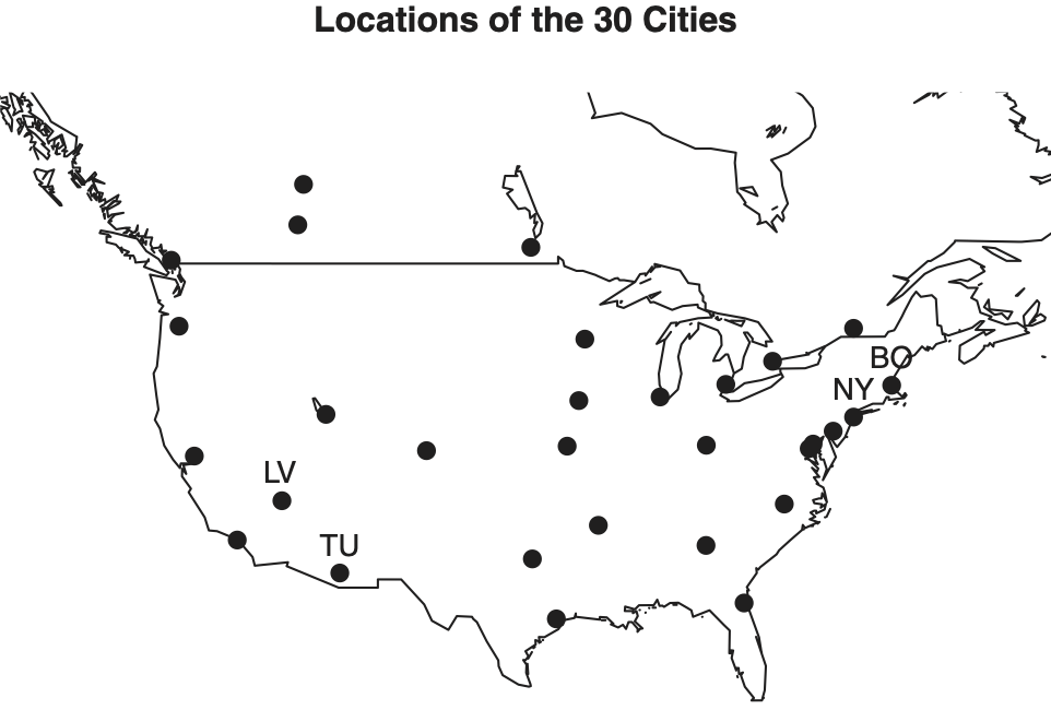
The temperature derivative described thus far applies to a single location. For multiple locations, one should realize that the financial performance of those locations are dependent, as the underlying weather variable could be dependent. In this paper we explore how the spatial dependence of temperature derivatives impacts financial risks. Currently, temperature derivatives are actively traded on the CME for 30 North American cities, whose locations are shown in Figure 1. Since the temperature at two nearby locations can be closely related, so too can the financial outcomes of temperature derivatives for those cities. Spatial dependence in weather derivatives has been explored in limited cases by Saltyte Benth, Benth, and Jalinskas (2007), Saltyte Benth and Saltyte (2011), and Erhardt and Smith (2014), but each paper considers limited cases. Here we aim to extend the reach of such cases by covering a wider class of temperature derivatives.

Figure 1.Locations of the 30 North American cities whose temperature derivatives are listed on the Chicago Mercantile Exchange. The four cities, Boston, New York, Las Vegas, and Tucson (which are highlighted throughout this paper), are labeled BO, NY, LV, and TU, respectively

In this paper, we develop a methodology for measuring the risk of holding an arbitrary portfolio of CME-traded temperature derivatives with a specific eye towards spatial dependence of locations. We take the point of view of a company which holds a portfolio of temperature derivatives, some of which will involve payments triggered by weather events. Whether the company directly sold the derivatives to various buyers or came to hold the obligations through trading is immaterial. What matters is the best estimate of combined risk from holding such a portfolio. Therefore the paper will focus on estimating risk measures for losses, and will not focus on the premium/revenue the company earned by accepting the risk in the first place.

Further, we explore quantifying the risk from temperature derivatives with an eye towards trends due to climate change. The fifth assessment report from the Intergovernmental Panel on Climate Change has been released (IPCC 2013), and it predicts global increases in average temperatures. It also states that “it is extremely likely that human influence has been the dominant cause of the observed warming since the mid-20th century.” Computer model experiments under different carbon emissions scenarios give projections of future temperature rise in line with future greenhouse gas emissions. The Bulletin of the American Meteorological Society called for “very long-term hedging contracts” to help manage climate risk (Dutton 2002). It seems likely that increasing concerns over climate change will continue to have an impact on temperature derivative markets, and climate trends must be incorporated into their study. The methodology described in this paper incorporates long-term trends in temperature due to climate change.

Weather risk markets have the potential to impact the way some insurance companies operate with regard to weather-related risks. Mills (2005) discussed the scope of climate change risk to the insurance industry. Erhardt and Smith (2014) explored a connection between weather derivatives, extremes, and insurance. Since the financial outcomes of weather derivatives are minimally correlated with other financial outcomes facing the insurance industry (Alexandridis and Zapranis 2013), investing in weather derivatives is one approach that an insurance company can take to maximize returns for a given risk level. Additionally, since the events which trigger a weather derivative payment arise from scientific laws governing the weather, the construction of probabilistic models for an actuarial method of pricing and measuring risk is possible (Jewson, Brix, and Ziehmann 2005).

2. The data and risk measures

2.1. Data

Daily temperature data were freely obtained from the National Climate Data Center (http://www.ncdc.noaa.gov/cdo-web/). Specifically, we obtained data for the 30 North American cities whose temperature derivatives are listed on the Chicago Mercantile Exchange. Locations of the cities are shown in Figure 1. At each location, measurements include the maximum daily temperature T_max and minimum daily temperature T_min in degrees Fahrenheit for the period January 1, 1945, through August 30, 2014. Although SI units are common in much of the world, the Chicago Mercantile Exchange lists all North American temperature derivatives in degrees Fahrenheit, so we follow this convention.

Let d = 1, . . . , D = 30 index the 30 cities, and let t be an index for time. Following the conventions used in weather derivative pricing (Jewson, Brix, and Ziehmann 2005; Alexandridis and Zapranis 2013), we define the daily observed temperature as

$$T_{\text {obs }}(d, t)=\frac{1}{2}\left(T_{\min }(d, t)+T_{\max }(d, t)\right).$$

For each day, cooling degree days are computed as

$$C D D(d, t)=\max \left(T_{o b s}(d, t)-65,0\right),$$

and heating degree days are computed as

$$\operatorname{HDD}(d, t)=\max \left(65-T_{o b s}(d, t), 0\right).$$

Cooling and heating degree days are most commonly used to construct cumulative indices over some time period of interest. Let $\{t \in \mathcal{T}\}$ be the set of all days within the time period of interest . Then a cumulative CDD index is simply

$$c C D D(d, \mathcal{T})=\sum_{t \in T} C D D(d, t),$$

where is a time period of interest—most commonly one of the calendar months, a set of adjacent months, or one of the six-month periods April 1–Sep 30 or October 1–March 31 (Jewson, Brix, and Ziehmann 2005). Six-month contracts are commonly traded, and have been studied in other papers (Campbell and Diebold 2005; Erhardt 2014).

2.2. Actuarial risk measures

It can be useful to imagine a company that sells derivatives to various buyers for some premium, and then holds these obligations as a risk—the hope is that the realization of this risk is less than the total revenue brought in at the sale. Call L the random loss that the institution will ultimately have to pay. The exact realization of L comes after the last settlement date has passed. The specific mathematical relationship linking this loss L to the degree-day settlement index (cCDD($\mathcal{T}$) or cHDD($\mathcal{T}$)) will be outlined in later sections. Here it suffices to see that L is simply a function based on the random variable temperature, T, and that one can therefore build up distributions of L by constructing distributions of temperature T and degree-day indices.

We will estimate values for various actuarial risk measures as defined in Kaas et al. (2008). Definitions for risk measures in the actuarial literature are not universally agreed upon, so care should be taken. The value at risk is defined as

$$\operatorname{VaR}(L ; \alpha)=Q_{\alpha}=\min \left\{Q: P\left(L \leq Q_{\alpha}\right) \geq \alpha\right\}. \tag{2}$$

The VaR is easily obtained since the loss L is often a continuous random variable for larger values of α, and therefore the distribution function F_L(l) = P(L ≤ l) is strictly increasing and has inverse distribution function F_L⁻¹. Then we simply have Q_α = F_L⁻¹(α). Kaas et al. (2008) define the conditional tail expectation as

$$\operatorname{CTE}_{\alpha}(L)=\mathbb{E}\left(L \mid L>Q_{\alpha}\right), \tag{3}$$

which is the expected loss conditional upon exceeding the VaR.

3. Long-term modeling of CDD and HDD indices

Here we will always refer to cumulative CDDs for the time period April 1–Sep 30, and cumulative HDDs for the time period October 1–March 31. These are two of the more commonly traded temperature derivatives on the CME (Campbell and Diebold 2005). Summing degree days over six months allows one to use the normal approximation, since the length of summation is substantially longer than the length of temporal dependence in the data. The methodology is therefore substantially simpler than that needed for modeling shorter time periods.

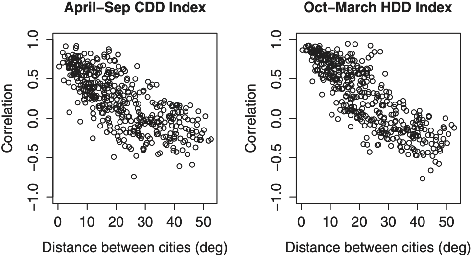
Figure 2 shows the October–March cHDDs for the four representative cities. For each city, the marginal distribution is roughly normal. Neighboring pairs Boston–New York and Las Vegas–Tucson each show strong positive dependence in cHDDs in the respective scatterplots, while non-neighboring pairs show little to no dependence, as expected. Figure 3 reinforces this point by plotting the linear correlation between two cities as a function of their geographic distance from one another (measured in degrees Lat-Lon). The general trend for both heating and cooling is high correlation at small distances, which drops off as distance increases.

Figure 2.October–March cumulative heating degree days for four representative cities. The neighboring pairs of Boston–New York and Las Vegas–Tucson show strong positive dependence, while pairs of cities much farther apart show little dependence

Figure 3.Linear correlation in the cCDDs and cHDDs as a function of the distance between the pairing of cities (measured in degrees)

Figures 4 and 5 highlight positive trends in cCDDs and negative trends in cHDDs over time at the four representative cities. These trends are a result of hotter summers and milder winters since the mid-twentieth century. For all 30 cities whose linear trends were significant at the 0.1 level, cCDDs and cHDDs were de-trended and put on a common year 2014 level. We did not de-trend data for a city whose trend estimates were not significant at the 0.1 level. Some statistical output for trend estimation is shown in Table 1.

Figure 4.Linear trends in the April–September cumulative cooling degree days for four representative cities. Slopes for Las Vegas and Tucson are significantly different from zero at the 0.05 level

Figure 5.Linear trends in the October–March cumulative heating degree days for four representative cities. Slopes for Las Vegas, New York, and Tucson are significantly different from zero at the 0.05 level

Readers may wonder about possible long distance spatial and/or temporal dependence introduced by climatic episodes such as El Niño, La Niña, the North Atlantic Oscillation, and other large-scale climatic phenomena. We investigated the possibility that historical cCDD and cHDD totals for some of the 30 cities should be adjusted using the Oceanic Niño Index (ONI) (http://www.cpc.ncep.noaa.gov/products/analysis_monitoring/ensostuff/ensoyears.shtml). Specifically, we calculated the April–October average ONI for the period 1950–2014, and compared this to the historical cCDDs for each of the 30 cities over the same time period. Similarly, we computed November–March average ONI values of the ONI and compared these to the cHDDs for each of the 30 cities from the period 1951–2014. We found no statistically significant trends or relationships that suggested an adjustment. This does not suggest that future research will not uncover statistical value in using climate indices such as the ONI as covariates. For example, it may be that there is a lag of several months between a high ONI value and its impact on North American temperature, and perhaps this temporal lag may differ for the 30 cities in North America based on their geographic location. All we state here is that the spatial dependence among locations is the largest omission to current actuarial temperature derivative pricing, and that further adjustments based on the ONI and similar indices are outside the scope of this paper. To recap, then, we have de-trended data for long-term climate trends but not any climate indices, and so the data x_i discussed in the next section always refer to the de-trended temperature values.

3.1. The model for cCDDs and cHDDs

The longest temporal autocorrelations observed for daily temperature data were about 14 days long. None of the cities showed any remaining temporal autocorrelation in annual indices from one year to the next. Since cumulative totals were computed by summing CDDs or HDDs over roughly 180+ days, these “long-term” indices were sufficiently long to produce normally distributed margins without autocorrelation by year. The natural choice for a model is to let X_i be the D = 30 dimensional random vector of cCDD (or cHDD) indices for year i = 1, . . . , n, and to model X_i as multivariate normal,

$$X \sim N\left(\mu_{X}, \Sigma_{X}\right),$$

where μ_X is the mean vector and $\Sigma_X$ is the covariance matrix. Readers familiar with spatial interpolation and kriging should recognize that our goal is only to model the dependence at the particular locations of the 30 cities listed on the CME; therefore, it isn’t necessary to choose a Gaussian process model, interpolate to unobserved locations, and so forth. The 30 by 30 dimension covariance matrix $\Sigma_X$ is easily invertible from a computational cost standpoint. The covariance is estimated with the usual unbiased estimator

$$\hat{\Sigma}_{X}=\frac{1}{n-1} \sum_{i=1}^{n}\left(x_{i}-\bar{x}\right)\left(x_{i}-\bar{x}\right)^{T}. \tag{4}$$

The mean of the multivariate normal is estimated using

$$\hat{\mu}_{X}=\frac{1}{n} \sum_{i} x_{i}. \tag{5}$$

4. Models for losses

4.1. Affine models

An affine transformation of random vector X is any function of the form a + BX. Since our model assumes that cumulative degree days X follow a multivariate Gaussian distribution with D dimensional mean vector μ_X and D by D covariance matrix $\Sigma_X$, then any affine transformations of X will similarly be Gaussian with only a change in the mean and variance. We begin by considering a simple weather derivative that pays $20 per contract per degree day, with the sign of the payment determined by an entry level. Mathematically, this payment is

$$P_{i}=20 n_{i}\left(X_{i}-E_{i}\right)=-20 n_{i} E_{i}+20 n_{i} X_{i},$$

where n_i is the number of contracts for city i, X_i is the settlement value of the cumulative degree day index, and E_i is the entry level for city i. For the affine model of payments, the entry level refers to the point at which the sign of payments changes from positive to negative. For these weather derivatives there is always a payment; we will consider the more common case where payments are either positive or exactly zero in the next subsection. The amount $20 is selected since standard contracts traded on the CME pay $20 per degree per contract. As a simple example, if a company held 100 Atlanta cCDD contracts for the April 1–October 31 period with entry level 2000 cCDDs, but the index ultimately settled at 2200 cCDDs, the company would lose 100 · 20 · (2200 − 2000) = 400,000.

Define vector c^T as

$$c^{T}=\left(-20 n_{1} E_{1}, \ldots,-20 n_{30} E_{30}\right),$$

and square matrix B as

$$B=\left(\begin{array}{cccc} 20 n_{1} & 0 & \cdots & 0 \\ 0 & 20 n_{2} & \cdots & 0 \\ \cdots & \cdots & \cdots & \cdots \\ 0 & 0 & \cdots & 20 n_{30} \end{array}\right)$$

Then we can express the payment vector P = c + BX, which is an affine transformation of vector X, which has a known multivariate normal distribution. The distribution of P is also multivariate normal, as

$$P \sim N\left(c+B \mu_{X}, B \Sigma_{X} B^{T}\right) . \tag{6}$$

The quantity which is ultimately of interest is $L=\Sigma_i P_i$, the total aggregate scalar loss. If we define vector b^T = (1, . . . , 1) we can write L = b^TP, which is again an affine transformation and therefore the distribution of L is normal as

$$L \sim N\left(b^{T}\left(c+B \mu_{X}\right), b^{T} B \Sigma_{X} B^{T} b\right)=N\left(\mu_{L}, \sigma_{L}^{2}\right),$$

where μ_L is the univariate mean of the loss, and σ²_L is the variance of the loss. Observe that one model fit to the CDD and HDD indices can be used to estimate financial outcomes for any arbitrary collection of temperature derivatives. Different collections will involve different choices of the user-selected quantities b, c, and B, but the terms μ_X and $\Sigma_X$ will be the same. Estimates of the mean and variance of the financial payments L are simply

$$\hat{\mu}_{L}=b^{T}\left(c+B \hat{\mu}_{X}\right)$$

and

$$\hat{\boldsymbol{\sigma}}_{L}^{2}=b^{T} \boldsymbol{B} \hat{\Sigma}_{X} B^{T} b.$$

The Value at Risk (defined in Equation 2) is estimated by

$$\widehat{\operatorname{VaR}}(L ; \alpha)=\hat{Q}_{\alpha}=\min \left\{Q: \Phi\left(\frac{Q-\hat{\mu}_{L}}{\hat{\sigma}_{L}}\right) \geq \alpha\right\},$$

where Φ(·) is the cumulative distribution function for the standard normal. A closed-form expression for the estimator of CTE_α(L) (which was defined in Equation 3) can be derived by recognizing it is simply the expectation of a truncated normal (Greene 2003),

$$\widehat{C T E}_{\alpha}(L)=\hat{\mu}_{L}+\frac{\hat{\sigma}_{L}}{1-\Phi\left(\frac{Q_{\alpha}-\hat{\mu}_{L}}{\hat{\sigma}_{L}}\right)} \phi\left(\frac{Q_{\alpha}-\hat{\mu}_{L}}{\hat{\sigma}_{L}}\right),$$

where $\phi(\cdot)$ is the standard normal density function.

4.2. Extending to strike values

While the previous subsection provided some nice mathematical results and a simple framework for estimating some risk measures, nearly all weather derivatives have a payment that is non-linear in relationship to degree day indices, and typically there are no negative payments. Instead, there is a large probability of a zero dollar payment which occurs when the strike is not exceeded. Here we show how the previous mathematical results can be used with a computational approach to consider weather derivatives whose payments are identically zero unless the entry level is exceeded by the degree day index. Mathematically, payments are

$$P_{i}=20 n_{i} \max \left(X_{i}-E_{i}, 0\right)$$

where n_i is the number of contracts for city i, X_i is the value the cumulative degree day index settles at, and E_i is the strike level for city i—the amount that, once exceeded, dictates that non-zero payments are triggered. The key difference from the affine model is that now, in the event that X_i ≤ E_i, the payment is zero instead of negative. Hence it is the distribution of P_i|P_i > 0 that is a continuous distribution, and the distribution of P_i itself is a mixed discrete-continuous distribution with a point mass at P_i = 0.

Recall that our ultimate interest is in the quantity L_iP_i. The nonlinearity of the payment P_i makes closed-form distribution functions of L difficult to compute, so instead we turn to a computational approach:

1. Simulate a realization P′ from the Gaussian distribution shown in Equation 6.

2. For i = 1, . . . , 30 define R_i′ = max (P_i′, 0). This is simply replacing negative elements of P′ with zero.

3. Compute L′ = ∑_iR_i′

4. Repeat steps (1) - (3) J times.

The result is a collection of J realizations of the random variable L, and from this distribution one can compute empirical estimates of all desired risk measures. In general J should be a very large number, in the hundreds of thousands or millions, which costs very little in terms of computational power. This output can be used to estimate risk measures as

$$\widehat{\operatorname{VaR}}(L ; \alpha)=w_{1} \cdot L_{[j]}+w_{2} \cdot L_{[j+1]} \tag{7}$$

where $j / J<\alpha<(j+1) / J, L_{[j]}$ is the j^th order statistic, and w₁ + w₂ = 1 are the weights (whose relevance vanishes as J→∞). The conditional tail expectation can be estimated as

$$\widehat{C T E}_{\alpha}(L)=\frac{1}{|\tau|} \sum_{j} L_{j} \cdot I_{\left\{L_{j}>\widehat{\operatorname{VaR}}(L ; \alpha)\right\}}, \tag{8}$$

where |τ| is the number of losses above $\widehat{\operatorname{VaR}}(L ; \alpha) \text { and } \mathrm{I}_{\left\{L_{j}>\widehat{\operatorname{VaR}}(L ; \alpha)\right\}}$ and $I_{\left\{L_{j}>\widehat{\operatorname{VaR}}(L ; a)\right\}}$ is the indicator function which takes value 1 when the argument holds, and 0 otherwise.

5. Results

Estimated mean vectors $\hat{\mu}_X$ and covariance matrixes $\hat{\Sigma}_X$ for both cCDDs and cHDDs are shown in Tables 2 and 3. Since these tables can be used with any choice of vectors c and matrix B, they contain all information needed to estimate aggregate losses for a collection of April–September cCDD and October–March cHDD temperature derivatives. Spatial dependence is naturally incorporated through the off-diagonal elements of $\hat{\Sigma}$. Recall that since the data were de-trended to 2014 levels, some recognition of climate change trends was also incorporated.

Here we demonstrate the approach to computing the risk measures for the aggregate loss on a portfolio of cCDDs using the strike model. Suppose an insurance company wishes to hold 100 contracts at each of the four cities highlighted in this paper (Boston, Las Vegas, New York, and Tucson). For each of these four cities, the strike level E_i will be 100 CDDs higher than average cCDD values taken from $\hat{\mu}_X$ in Table 2. Thus, the four strike levels are 865, 3723, 1148, and 3442. We have selected strike values above the means for these four cities to demonstrate how zero dollar payments arise when none of the cities exceeds their respective strike values. To clarify, the company will pay amounts 20 100 max(X_i – E_i, 0). The total loss is obtained by adding the individual losses, but a closed-form density for L is not easily obtained so we will use the simulation based approach in Section 4.2, beginning with simulations of P. Specifically, the formulation of the multivariate normal distribution of P is:

• n_i = 100 for i = 3,13,17, and 23, and 0 otherwise;

• E₃ = 865; E₁₃ = 3723; E₁₇ = 1148; E₂₃ = 3442; E_i = 0 for all i not equal to 3,13,17,23

• The vector c = {c_i, i = 1, . . . , 30} has non-zero entries only for c₃ = −20 · n₃ · E₃ = −1,730,000; c₁₃ = −7,446,000; c₁₇ = −2,296,000; c₂₃ = −6,884,000.

• The matrix B has non-zero entries only for B_3,3 = B_13,13 = B_17,17 = B_23,23 = 20 · 100 = 2000.

• $\hat{\mu}_X$ and $\hat{\Sigma}_X$ are as shown in Table 2.

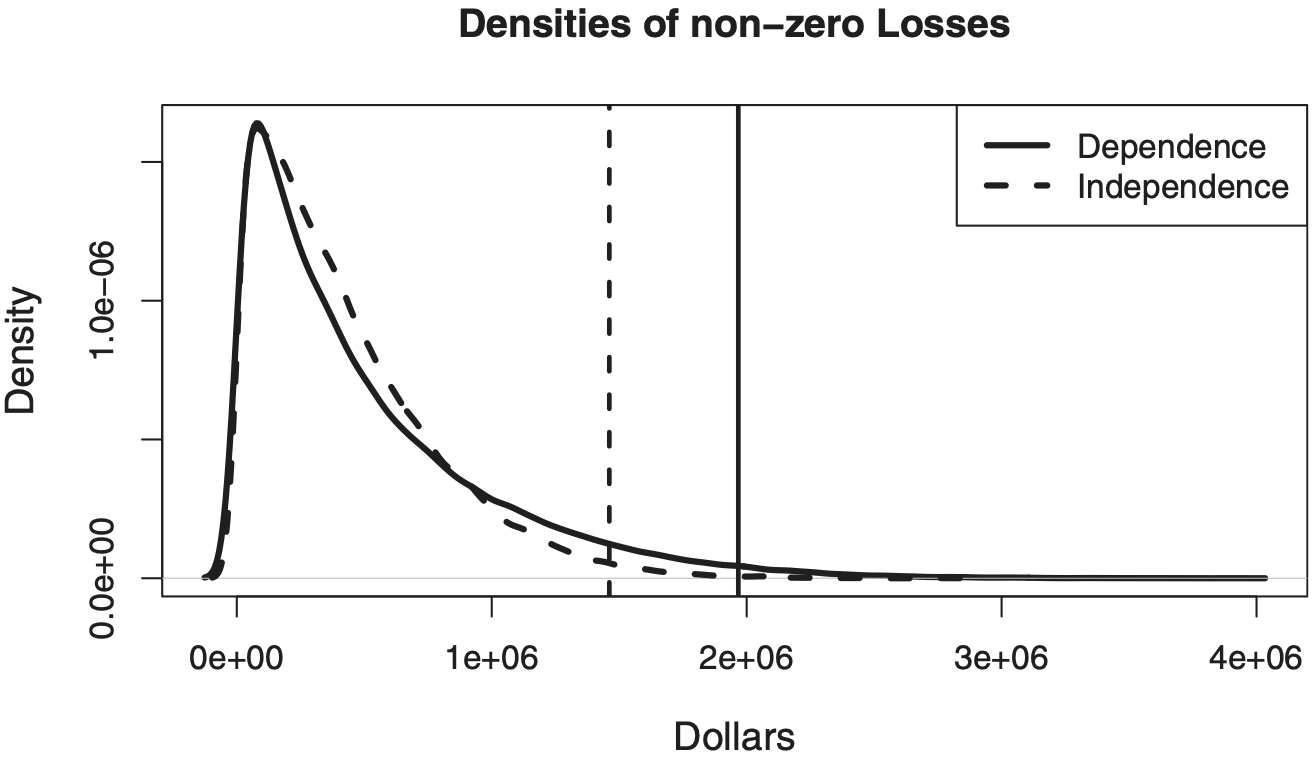
Thus, we have fully specified the multivariate Gaussian in Equation 6. We use this distribution to simulate J = 100,000 realizations, and for each realization we replaced negative elements with zero, producing what we termed R′ in Section 4.2. Total losses were the sum of the payments for each of the 100,000 realizations. In these simulations, fully 36.1% of payments were identically equal to zero, meaning that none of the four cities exceeded the respective strike values. The density of the remaining 63.9% of non-zero payments is shown in Figure 6 as the solid line. For comparison, we repeated the methodology ignoring spatial dependence (i.e., we set all off-diagonal terms of $\hat{\Sigma}_X$ to zero), and termed this the independence case. Here 24.2% of payments were identically zero, and the dashed line shows the density of the remaining 75.8% of non-zero payments. As expected, the variability and tail thickness of the dependent solid line is larger than for the dashed independent line. The 99th percentiles are also shown, and as expected the dependent case shows a much larger high percentile. Risk measures are shown in Table 4.

Figure 6.Empirical density estimates of non-zero losses using the strike value method described in section 4.2. The dependence distribution was built recognizing dependence among the four cities, while the independence distribution simulates independent losses for the four cities. Vertical dashed and solid lines show the 99th percentiles for the two cases

6. Discussion

In this paper we fit models for cumulative heating and cooling degree days for 30 North American cities. Through the use of a multivariate normal distribution, we incorporated spatial dependence among the 30 cities. Through affine transformations of cCDDs and cHDDs, we constructed normal distributions for payments and demonstrated how this distribution could be used to estimate some common risk measures. For the far more commonly traded derivatives based on a strike value, we demonstrated how a computational approach can simulate large numbers of losses and associated risk measures.

We demonstrated that historical data on degree day indices shows evidence of climate change consistent with scientific papers documenting the changes, and found statistically significant positive trends for cCDDS over the summer and statistically significant negative trends for cHDDs over the winter. Statistical models which use data going back several decades should explicitly recognize these trends and de-trend all data to the common time period of interest. Otherwise, models run the risk of slightly underestimating cCDDs and overestimating cHDDs. As mentioned earlier in the paper, we briefly investigated the need to adjust historical data based on El Niño and other climate oscillations but did not identify statistically significant relationships. We leave it as an open question to what degree incorporating external covariates based on climate indices would improve modeling.

A financial interest for the insurance industry comes about by recognizing that weather is minimally correlated with financial and insurance markets, and as such, the financial performance of weather derivatives is largely independent from the financial performance of other assets an insurer holds. This allows diversification and risk control. A business interest is simply that weather products can be new insurance products. Some property and casualty insurers are already in the business of selling insurance products to cover losses triggered from environmental or weather causes (crop, flood, and catastrophe insurance, to name only three). Sophisticated ratemaking procedures can incorporate past weather data and/or seasonal weather forecasting. A natural extension of this expertise might be found in weather products.

The most notable limitation of the method in this paper is its reliance on sufficiently long time periods to allow for normality in the degree day sums. We do not recommend this approach for modeling cumulative degree days over time periods too short to allow the normal approximation to hold. Specifically, we do not recommend this approach for a month or even a few months. To model degree day totals for shorter time periods, a fundamentally different approach must be used. An obvious choice would be to first model temperature at the daily level, and then use these models to construct distributions cCDDs and cHDDs. Closed-form solutions would likely be hard to come by given the model complexity required for daily temperatures, so a simulation-based approach may be needed. Such approaches are beyond the scope of this paper, but we mention them not only to highlight the limitation of the approach presented here for shorter time scales, but also to suggest future avenues of promising research.

Acknowledgments

The author wishes to thank the Research Grants Task Force of the Casualty Actuarial Society and the Committee on Knowledge Extension Research of the Society of Actuaries for their generous financial support of this project. The authors also wish to thank the two anonymous referees and the editorial staff of Variance for their helpful suggestions which improved the paper.