Dependencies in Stochastic Loss Reserve Models

1. Introduction

Recent attempts to apply enterprise risk management principles to insurance have placed a high degree of importance using stochastic models to quantify the uncertainty on the various estimates. For general insurers, the most important liability is the reserve for unpaid losses. Over the years, a number of stochastic models have been developed to address this problem. Some of the more prominent nonproprietary models are those of Mack (1993, 1994), England and Verrall (2002) and Meyers (2015).

As good as these models may be, they fall short of quantifying the uncertainty in the insurer’s liability as they do not address the issue of correlation (or more generally—dependencies) between lines of insurance. The failure to resolve this problem analytically has resulted in judgmental adjustments to various risk-based capital formulas. Herzog (2011) provides a summary of some current practices.

Zhang and Dukic (2013) describe what I believe to be a very good attempt at solving this problem. As this paper uses their paper as a starting point, it would be good to provide an outline of their approach.^[1]

But first, we need to set our notation. Let C^X_wd be the cumulative paid claim amount in line of insurance X for accident year, w = 1,. . . . , K and development year d = 1, . . . , K. Since this paper works with Schedule P data taken from the CAS Loss Reserve Database,^[2] we can set K = 10. In this paper, X will be CA for Commercial Auto, PA for Personal Auto, WC for Workers Compensation, or OL for Other Liability.

Now suppose that we have models for two different lines of insurance such as

$$\begin{array}{l} \log \left(C_{w d}^{X}\right) \sim \operatorname{Normal}\left(\mu_{w d}^{X}, \sigma_{d}^{X}\right) \\ \log \left(C_{w d}^{Y}\right) \sim \operatorname{Normal}\left(\mu_{w d}^{Y}, \sigma_{d}^{Y}\right) \end{array} \tag{1.1}$$

As we shall see below, the parameters μ^X_wd will be functions of w and d and the parameters σ^X_d will be subject to constraints for each line X. That feature can be ignored for now as we are setting up the problem.

As shown in Meyers (2015), it is possible to use a Bayesian MCMC model to generate a large sample, say of size 10,000, from the posterior distributions of $\left\{\left\{{\mathstrut}_i \mu_{w d}^X\right\},\ \left\{{\mathstrut}_i \sigma_d^X\right\}_{i=1}^{10000}\right.$ for each line of insurance X.

The idea put forth by Zhang and Dukic is to fit a bivariate Bayesian MCMC model of the following form, given the Bayesian MCMC models described by Equation (1.1).

$$\begin{array}{l} \binom{\log \left(C_{w d}^{X}\right)}{\log \left(C_{w d}^{Y}\right)} \sim \text { Multivariate Normal } \\ \left(\binom{\mu_{w d}^{X}}{\mu_{w d}^{Y}},\left(\begin{array}{cc} \left(\sigma_{d}^{X}\right)^{2} & \sigma_{d}^{X} \cdot \rho \cdot \sigma_{d}^{Y} \\ \sigma_{d}^{X} \cdot \rho \cdot \sigma_{d}^{Y} & \left(\sigma_{d}^{Y}\right)^{2} \end{array}\right)\right) \end{array} \tag{1.2}$$

The correlation parameter, ρ, describes the dependency between Line X and Line Y.

Zhang and Dukic then use a Bayesian MCMC model to obtain a large sample from the posterior distribution:

$$\left\{\left\{\begin{array}{c} {\mathstrut}_{i} \mu_{w d}^{X *} \\ {\mathstrut}_{i} \mu_{w d}^{Y *} \end{array}\right\},\left\{\begin{array}{cc} \left({\mathstrut}_{i} \sigma_{d}^{X *}\right)^{2} & {\mathstrut}_{i} \sigma_{d}^{X *} \cdot{\mathstrut}_{i} \rho \cdot{\mathstrut}_{i} \sigma_{d}^{Y *} \\ {\mathstrut}_{i} \sigma_{d}^{X *} \cdot{\mathstrut}_{i} \boldsymbol{\rho} \cdot{\mathstrut}_{i} \boldsymbol{\sigma}_{d}^{Y *} & \left({\mathstrut}_{i} \sigma_{d}^{Y *}\right)^{2} \end{array}\right\}\right\}_{i=1}^{10000}$$

The asterisk (*) on the μ and σ parameters calls attention to the fact that the posterior distributions from the models in Equation (1.1) may, and often do, differ significantly from the corresponding marginal posterior distributions from the models in Equation (1.2). To the actuary who prepares loss reserve reports, this presents a problem. Typically, actuaries analyze their reserves by individual line of insurance. With a Bayesian MCMC model, they can quantify the uncertainty of the outcomes for that line. Now suppose that there is a demand to quantify the uncertainty in the sum of losses for two or more lines of insurance using the Zhang-Dukic framework. They will need to explain, for example, why the univariate distribution for Commercial Auto produces different results than the marginal distribution for Commercial Auto when combined with Personal Auto. And the marginal distribution could be different still when combined with Workers Compensation.

Scalability is also a problem. For example, the univariate model used in this paper has 31 parameters. Using this model with the bivariate Zhang-Dukic framework yields a model with 31 + 31 + 1 = 63 parameters. In theory, Bayesian MCMC software can handle it, but in practice I have found that running times increase at a much faster rate than the number of parameters. I have coded models using the bivariate Zhang-Dukic framework that work well for some pairs of loss triangles, but others took several hours of running time to obtain convergence of the MCMC algorithm.

The purpose of this paper is to present a framework similar to that of Zhang and Dukic that preserves the univariate models as the marginal distributions.

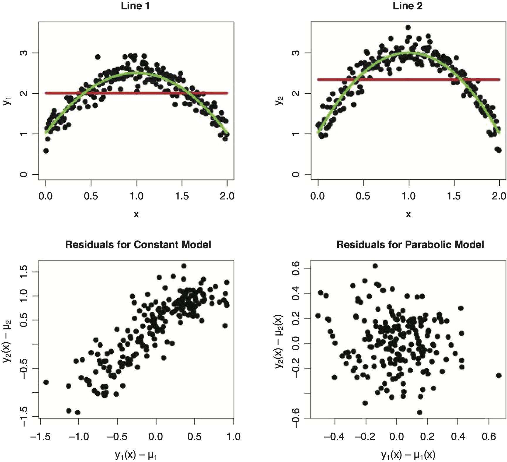
Before we go there, we should note that a suboptimal model might produce artificial dependencies. To illustrate, consider Figure 1.1, where y₁ and y₂ are independent random deviations off two parabolic functions of x. We want to fit a bivariate distribution to the ordered pair (y₁(x), y₂(x)) of the form:

$$\begin{array}{l} \binom{y_{1}}{y_{2}} \sim \text { Multivariate Normal } \\ \left(\binom{\mu_{1}}{\mu_{2}},\left(\begin{array}{cc} \sigma_{1}^{2} & \sigma_{1} \cdot \rho \cdot \sigma_{2} \\ \sigma_{1} \cdot \rho \cdot \sigma_{2} & \sigma_{2}^{2} \end{array}\right)\right) \end{array}\tag{1.3}$$

Figure 1.1.Illustration of artificial correlation

The upper plots of Figure 1.1 show the pairs (x, y₁(x)) and (x, y₂(x)) with the suboptimal constant models plotted in red, and the correct parabolic models plotted in green. The lower left plot shows a scatter plot of y₁(x) − μ₁ and y₂(x) − μ₂ for the suboptimal model. The lower right plot is a scatter plot of y₁(x) − μ₁(x) and y₂(x) − μ₂(x) for the correct parabolic model. This example shows how suboptimal models for the marginal distribution can cause an artificial nonzero correlation the multivariate model. Avanzi, Taylor, and Wong (2016) discuss this phenomenon in greater detail.

The next section will describe the data used in this paper. Section 3 will describe the univariate (marginal) models and illustrate some diagnostics to test the appropriateness of the model. Section 4 will show how to obtain a random sample from the posterior distribution of parameters subject to the constraint that the marginal distribution is the same as those obtained by the corresponding univariate models. Section 5 will describe statistical tests to test the hypothesis that the correlation parameter, ρ, in the bivariate distribution is significantly different from zero. Section 6 will address the sensitivity of the results to the choice of models, and Section 7 will discuss the conclusions.

This paper assumes that the reader is familiar with Meyers (2015).

2. The data

The data used in this paper comes from the CAS Loss Reserve Database.^[3] The Schedule P loss triangles taken from this database are listed in Appendix A of Meyers (2015). There are 200 loss triangles, 50 each from the CA, PA, WC and OL lines of insurance. Univariate models from all 200 loss triangles will be analyzed in Section 3 and 6.

At the time of writing the monograph (Meyers 2015), I did not envision a dependency study. But it turned out that there were 102 within-group pairs of triangles (29 CA-PA, 17 CA-WC, 17 CA-OL, 14 PA-WC, 15 PA-OL and 10 WC-OL) that were suitable for studying dependency models. Preferring to use loss triangles that had already been vetted, I decided to stick with these within-group pairs of triangles.

This paper will provide detailed analyses for two illustrative insurers (Group 620 - Lines CA and PA and Group 5185 Lines CA and OL). The complete loss triangles and outcomes are in Table 2.1. The upper data triangle used to fit each model is printed with the ordinary font. The lower data triangle used for retrospective testing is printed with bold and italicized font.

A complete list of the insurer groups used in this paper is included in a zip archive titled “Appendix.” The files in the Appendix contain:

• The 200 groups along with the univariate model calculations in Sections 3 and 6.

• The R scripts that produce the univariate model calculations described in Section 3 and 6.

• The 102 within-group pairs with the bivariate model calculations in Sections 4, 5 and 6.

• The R scripts that produce the bivariate model calculations described in Sections 4, 5 and 6.

3. The changing settlement rate (CSR) model

The univariate model used in this paper will be a minor modification to the CSR model used in Meyers (2015). Here is the model. Let:

1. $\alpha_{w} \sim \operatorname{Normal}(0, \sqrt{10})$ for w = 2, . . . ,10. α₁ = 0.

2. logelr ∼ Uniform(−1, 0.5).

3. $\beta_d$ ∼ Uniform(−5, 5) for d = 1, . . . ,9. β₁₀ = 0.

4. S₁ = 1, S_w = S_w−1 • (1 − γ − (w − 2) • δ) for w = 2, . . . ,10. γ ∼ Normal (0, 0.05), δ ∼ Normal(0, 0.01).

5. $\mu_{w d}=\log \left(\operatorname{Premium}_w\right)+ logelr+\alpha_w+\beta_d \cdot S_w$.

6. $\sigma_{d}^{2}=\sum_{i=d}^{10} a_{i}$a_i ∼ Uniform(0, 1).

7. $\log \left(C_{w d}\right) \sim \operatorname{Normal}\left(\mu_{w d}, \sigma_d\right)$.

This model differs from the CSR model described in Meyers (2015) in three aspects.

1. The parameter γ allows for a speedup (or slowdown when γ is negative) of the claim settlements. By including the δ parameter, this version of the CSR model allows the settlement rate to change over time.

2. Forcing α₁ = 0 eliminates some overlap between the $\alpha_w$ parameters and the logelr parameter. In the Meyers (2015) version of the model, a constant addition to each $\alpha_w$ parameters could be offset by a subtraction in the logelr parameter. Correcting features of this sort tends to speed up convergence of the MCMC algorithm.

3. The MCMC software used for the calculation described in this paper is Stan. See http://mc-stan.org for installation instructions. I have found that, in general, the MCMC algorithm implemented by Stan converges faster than that of JAGS. Stan also allows one to compile a model (in C++) in advance of its use. Using a compiled model can greatly speed up the processing when one uses the same model repeatedly (as we will do below) with different inputs.

The R script that implements this version of the CSR model is available in the appendix spreadsheet. The script produces a sample from the posterior distribution of the parameters for line X,

$$\left\{\begin{array}{c} \left\{{\mathstrut}_i \alpha_w^X\right\}_{w=2}^{10},\left\{{\mathstrut}_i \beta_d^X\right\}_{d=1}^9,\left\{{\mathstrut}_i \sigma_d^X\right\}_{d=1}^{10}, \\ {\mathstrut}_i logelr^X, {\mathstrut}_i \gamma^X,{\mathstrut}_i \delta^X \end{array}\right\}_{i=1}^{10000}$$

Following Meyers (2015), the script then simulates 10,000 outcomes {_iC^X_w,10}_i=1¹⁰⁰⁰⁰ from which we can calculate various summary statistics such as the predictive mean and standard deviation of the outcomes and the percentile of the actual outcome. Table 3.1 gives a summary of the result of these calculations for the illustrative insurers in their two lines of business.

Figure 3.1 gives the test for uniformity of the predictive percentiles of this version of the CSR model. When compared with Meyers (2015) Figure 22, we see that allowing the claim settlement rate to change over time improves the model so that the percentiles are (within 95% statistical bounds) uniformly distributed for all four lines.

Figure 3.1.Uniformity tests for CSR model

Figure 3.1.Uniformity tests for CSR model (continued)

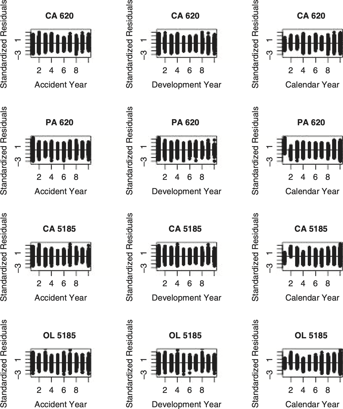
While the observation that the CSR model performs well on a large number of old triangles with outcome data is encouraging, it should not relieve the actuary from testing the assumptions underlying their model of their current data. Traditional tests, such has those provided by Barnett and Zehnwirth (2000), plot residuals (i.e., differences between observed and expected values) along accident year, development year and calendar year dimensions.

The Bayesian MCMC models in this paper provide a sample of size 10,000 from a posterior distribution of parameters. Given that we have this large sample, I consider it to be more informative if we take a subsample, S, of (say) size 100, then calculate the standardized residuals for each w and d in the upper loss triangle, and s in the subsample

$$R_{S}^{X}=\left\{\frac{\log \left(C_{w d}^{X}\right)-{\mathstrut}_{s} \mu_{w d}^{X}}{{\mathstrut}_{s} \sigma_{d}^{X}}\right\}_{s \in S} \tag{3.1}$$

In general we should expect these residual plots to have a standard normal distribution with mean 0 and standard deviation 1. Figure 3.2 shows plots of these standardized residuals against the accident year, development year and calendar year for the illustrative insurers. I have made similar plots for other insurers as well. For accident years and development years, the plots have always behaved as expected. Deviations for the early calendar years as shown in two of the four plots are not uncommon. I have chosen to regard them as unimportant, and attach more importance to later calendar years.

Figure 3.2.Standardized residual plots for the CSR model

If the standardized residual plots look like those of the illustrative insurers, we should not have to worry about artificial correlations.

4. Fitting bivariate distributions

The previous section presented a univariate model that performed well on data in the CAS Loss Reserve Database. This section shows how to construct a bivariate distribution with the CSR model as marginal distributions.

To shorten the notation let

$${\mathstrut}_{i} \theta^{X}=\left\{\begin{array}{c} \left\{{\mathstrut}_{i} \boldsymbol{\alpha}_{w}^{X}\right\}_{w=2}^{10},\left\{{\mathstrut}_{i} \beta_{d}^{X}\right\}_{d=1}^{9},\left\{{\mathstrut}_{i} \boldsymbol{\sigma}_{d}^{X}\right\}_{d=1}^{10} \\ {\mathstrut}_{i} \operatorname{logelr}{\mathstrut}^{X},{\mathstrut}_{i} \gamma^{X},{\mathstrut}_{i} \delta^{X} \end{array}\right\}$$

for line X and i = 1, . . . ,10000.

Let’s first consider what happens when we try the Zhang-Dukic approach with the CSR model. Let’s call this model the ZD-CSR model. Using Bayesian MCMC to get a sample from the posterior distribution for X=CA and Y=PA of Insurer #620 yields:

$$\left\{{\mathstrut}_{i} \theta^{C A}, \theta_{i}^{P A}, \rho_{i} \mid\left\{C_{w d}^{C A}\right\},\left\{C_{w d}^{P A}\right\}\right\}_{i=1}^{10,000}$$

The prior distributions for the _iθ^X parameters are the same as they are for the CSR model. The prior distribution for the ρ parameter is a β(2,2) prior distribution translated from (0,1) to (−1,1).

Using the parameter sets

$$\left\{{\mathstrut}_{i} \theta^{C A}\right\}_{i=1}^{10,000} \text { and }\left\{{\mathstrut}_{i} \theta^{P A}\right\}_{i=1}^{10,000}$$

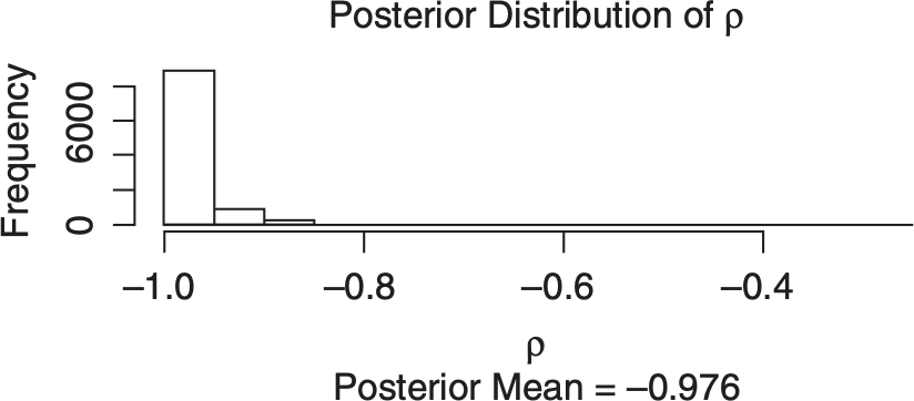
I then simulated the marginal distributions, given in Table 4.1, for each line of insurance. Notice that the estimates and the standard deviations are significantly higher for marginal distributions of the ZD-CSR model than for the corresponding univariate distributions in Table 3.2. Moreover, the posterior distribution of ρ in the ZD-CSR model, given in Figure 4.1, appears be clustered close to negative 1. This suggests that something is wrong with the ZD-CSR model.

Figure 4.1.The posterior distribution of $\rho$ for the ZD-CSR model

One way I found to improve the ZD-CSR model is to allow the correlation parameter, ρ, to vary by settlement lag. Let’s call this model the ZD2-CSR model.

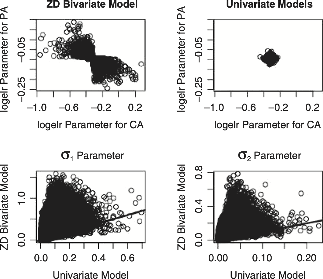
Figure 4.2 shows that the $\rho_d$s vary by settlement lag. Table 4.2 shows that the marginal distributions implied by the ZD2-CSR model are much closer to the univariate distributions in Table 3.1. Outputs from the ZD2-CSR model for other insurers show similar results, but the pattern of the $\rho_d$s are quite different. For some insurers the $\rho_d$s are predominantly positive. Regardless of whether or not the $\rho_d$s are positive or negative, the “outlier” $\rho_d$s usually appear at different settlement lags.^[4]

Figure 4.2.Boxplot of posterior distribution of $\rho_d$s for ZD2-CSR model

This erratic behavior of the $\rho_d$s suggests that a good practice would be to force those $\rho_d$s to be equal for all settlement lags. This is what the ZD-CSR model does! This model forces the other parameters to account for the differences in the data that indicate differing $\rho_d$s in the ZD2-CSR model. It turns out that the differences in the parameters are quite large. Figure 4.3 shows the differences between some of the parameters in the bivariate and the univariate models. If we are to produce a model that has a single ρ parameter, we need to find a way to preserve the marginal distributions produced by the univariate models.

Figure 4.3.Selected parameter comparisons for ZD-CSR and univariate models

Let’s now move on to a two-step approach that produces a bivariate model that preserves the univariate distributions as the marginal distributions.

The first step is to obtain the univariate samples, $\left\{{\mathstrut}_i \theta^X \mid\left\{C^X{\mathstrut}_{w d}\right\}\right\}_{i=1}^{10,000}$ and $\left\{{\mathstrut}_i \theta^Y \mid\left\{C^Y{\mathstrut}_{w d}\right\}\right\}_{i=1}^{10,000}$ where C^X_wd Upper Triangle of line X and C^Y_wd Upper Triangle of line Y. Then repeatedly for each i, use Bayesian MCMC to take a sample from the posterior distribution of {ρ|{C^X_wd}, {C^Y_wd}, _iθ^X, _iθ^Y} where ρ has a β(2,2) prior distribution translated from (0,1) to (−1,1). Next we randomly select a single _i ρ from that sample and use $\left\{{\mathstrut}_i \theta^X,{\mathstrut}_i \theta^Y,{\mathstrut}_i \rho\right\}_{i=1}^{10,000}$ to calculate the derived parameters in the bivariate distribution given by Equation (1.2). This amounts to using the two univariate distributions as the prior distribution for the second Bayesian step. From that two-step bivariate distribution, one can simulate outcomes from the “posterior” distribution of parameters and calculate any statistic of interest. Be reminded that this can be different from the usual Bayesian posterior distribution $\left\{{\mathstrut}_i \theta^X,{\mathstrut}_i \theta^Y,{\mathstrut}_i \rho \mid\left\{C_{w d}^X\right\},\left\{C_{w d}^Y\right\}\right\}_{i=1}^{10,000}$ that comes out of the Zhang-Dukic approach.

At first glance, one might expect the run time for 10,000 Bayesian MCMC simulations to be unacceptably long. But there are a number of considerations that allow one to speed up the calculations.

1. The MCMC simulation is for a single parameter that runs much faster than a multi-parameter simulation that one normally runs with stochastic loss reserve models.

2. We have a good starting value, _i ρ = 0. The burn-in period is short and convergence is rapid.

3. Since we are repeatedly running the same model with different inputs, we need only compile the model once, which the Stan software permits.

4. Using the “parallel” package in R allows one to distribute the simulations to separate cores on a multi-core computer.

Taking these factors into account, my fairly new high-end laptop usually turns out this bivariate distribution in about 5 minutes. As I mentioned above, the R scripts that produce these calculations are made available to the reader in the Appendix.

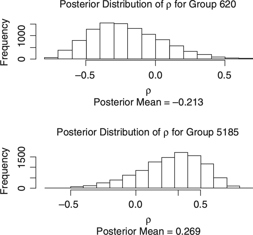
The purpose of getting a bivariate distribution is to predict the distribution of the sum of the outcomes for the two lines of insurance. Table 4.3 gives results analogous to Table 3.1 for the sum of the two lines for the two illustrative insurers. Also included are the sums of the two lines predicted under the assumption of independence. Figure 4.4 contains histograms of the two-step posterior distributions for ρ for the illustrative insurers.

Table 4.3 and Figure 4.4 are notable in two aspects. First, the output from the bivariate model is not all that different from the output created by taking independent sums of losses from the univariate model. Second, the posterior distributions of ρ from the two-step bivariate model have a fairly wide range.

Figure 4.4.Posterior distribution of $\rho$ for CSR 2-step bivariate model

Typically, the posterior mean ρ over all the within-group pairs of lines is not all that different from zero. Figure 4.5 shows the frequency distribution of posterior mean ρs from the insurer group sample.

Figure 4.5.Posterior mean $\rho$s from the 102 within-group pairs of lines

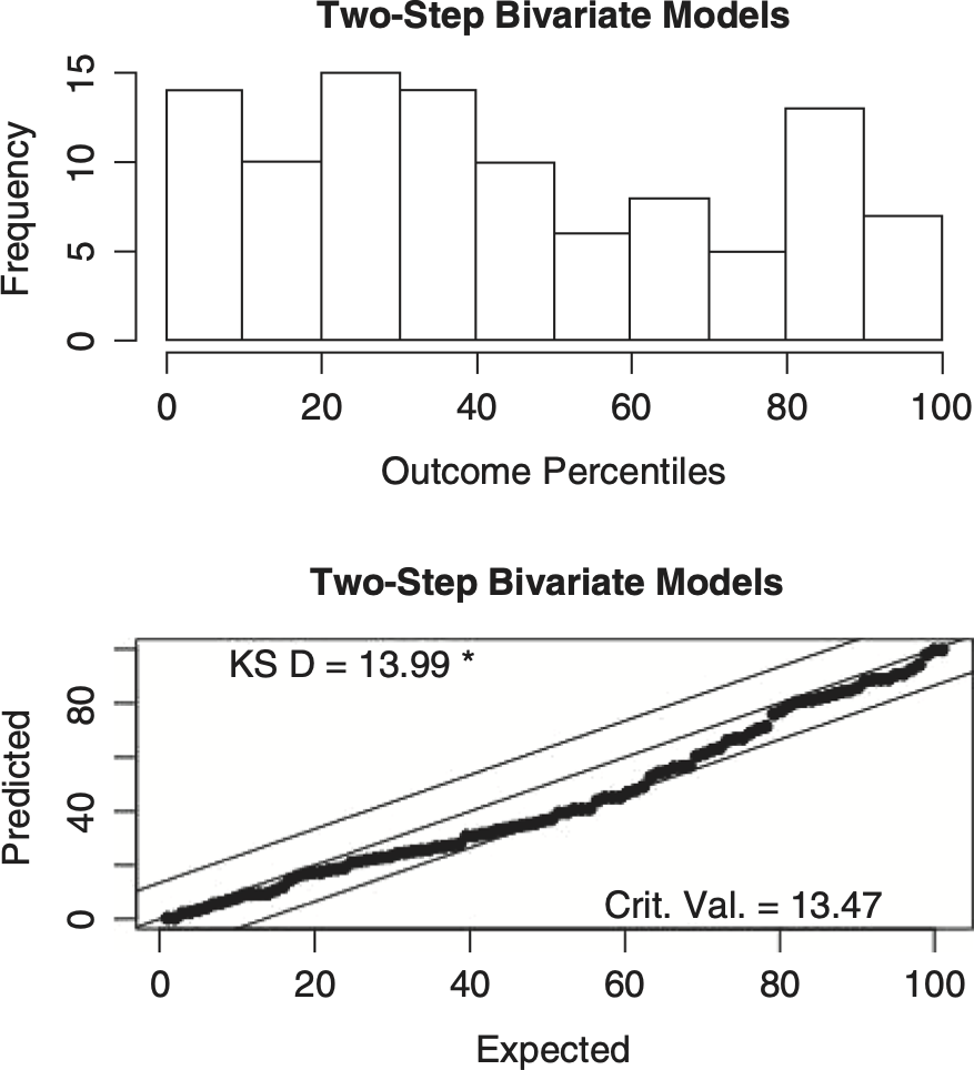
This section concludes with a test of uniformity of the outcome percentiles of the within-group pairs for the sum of two lines predicted by the two-step bivariate model and the independence assumption. As Figure 3.1 shows, the univariate models pass our uniformity test, so one would think that a valid bivariate model would also pass a uniformity test. Figures 4.6 and 4.7 show the results.

Figure 4.6.Uniformity tests of outcome percentiles

Figure 4.7.Uniformity tests of outcome percentiles

It turns out that the two-step bivariate model just barely fails the test and the independence assumption passes the uniformity test. This suggests that the lines of insurance are independent for many, if not all, insurers. In the next section we will examine the independence assumption for individual pairs of loss triangles.

5. Model selection

Let’s start the discussion with a review of the Akaike information criteria (AIC).

Suppose that we have a model with a data vector, x, and a parameter vector θ, with p parameters. Let ϑ̂ be the parameter value that maximizes the log-likelihood, L, of the data, x = {x_j}^J_j=1}. Then the AIC is defined as

$$\mathrm{AIC}=2 \cdot p-2 \cdot L(\mathbf{x} \mid \hat{\vartheta}) \tag{5.1}$$

Given a choice of models, the model with the lowest AIC is to be preferred. This statistic rewards a model for having a high log-likelihood, but it penalizes the model for having more parameters.

There are problems with the AIC in a Bayesian environment. Instead of a single maximum likelihood estimate of the parameter vector, there is an entire sample of parameter vectors taken from the model’s posterior distribution. There is also the sense that the penalty for the number of parameters should not be as great in the presence of strong prior information.

To address these concerns, Gelman et al. (2014, Chapter 7) describe statistics that generalize the AIC in a way that is appropriate for Bayesian MCMC models.^[5] Here is a brief overview of two of these statistics.

First, given a stochastic model p(x|ϑ), define the log of predictive point density as

$$\text { elpd }=\sum_{j=1}^{J} \log \left(\int p\left(x_{j} \mid \vartheta\right) \cdot f(\vartheta) d \vartheta\right) \tag{5.2}$$

where f is the unknown density function of ϑ.

If {_iϑ}^I_i=1, is a sample from the posterior distribution of ϑ, define the computed log predictive density as

$$\widehat{l p d}=\sum_{j=1}^{J} \log \left(\frac{1}{I} \sum_{i=1}^{I} p\left(\left.x_{j}\right|_{i} \vartheta\right)\right) \tag{5.3}$$

Note that if we replace {_iϑ}^I_i=1 with the maximum likelihood estimate, $\widehat{l p d}$ is equal to L(x|ϑ̂) in Equation (5.1).

If the data vector, x, comes from a holdout sample, i.e., x was not used to generate the parameters {_iϑ}^I_i=1, then $\widehat{l p d}$ is an unbiased estimate of elpd.

But if the data vector, x, comes from the training sample, i.e., x was used to generate the parameters {_iϑ}^I_i=1, then we expect that $\widehat{l p d}$ will be higher than elpd. The amount of the bias is called the “effective number of parameters.”

With the above as a high-level view, let’s first consider what is called “leave one out cross validation” or “loo” for short. For each data point x_k, one obtains a sample of parameters {_iϑ^(−k)}^I_i=1 by an MCMC simulation using all values of x except x_k. After doing this calculation for all observed data points {x_k}^J_k=1 one can then calculate an unbiased estimate of elpd

$$\widehat{e l p d}_{\text {loo }} \equiv \widehat{\operatorname{lpd}}_{\text {loo }}=\sum_{k=1}^{J} \log \left(\frac{1}{I} \sum_{i=1}^{I} p\left(\left.x_{k}\right|_{i} \boldsymbol{\vartheta}^{(-k)}\right)\right) . \tag{5.4}$$

The effective number of parameters is then given by $\hat{p}_{l o o} \equiv \widehat{l p d}-\widehat{e l p d}_{l o o} \text {. }$

As is done with the AIC in Equation (5.1), we can express $\widehat{e l p d}_{\text {loo }}$ on the deviance scale by writing

$$\mathrm{LOO}-\mathrm{IC}=-2 \cdot \widehat{e l p d}_{l o o}=2 \cdot \hat{p}_{l o o}-2 \cdot \widehat{l p d}_{l o o} \text {. } \tag{5.5}$$

When comparing two models, the model with the higher $\widehat{\text { elpd }}_{\text {loo }}=\widehat{l p d}_{\text {loo }}-\hat{p}_{\text {loo }}$, or equivalently, the model with the lower LOO-IC should be preferred.

Our second model selection statistic, called the Watanabe-Akaike information criteria (WAIC), is calculated using only the training data, x = {x_j}^J_j=1. Following Gelman et al. (2014) this statistic is given by

$$\widehat{e l p d}_{\text {waic }}=\widehat{l p d}-\hat{p}_{\text {waic }} \tag{5.6}$$

where^[6]

$$\hat{p}_{\text {waic }}=\sum_{j=1}^{J} \operatorname{Var}\left[\left\{\log \left(p\left(\left.x_{j}\right|_{i} \vartheta\right)\right)\right\}_{i=1}^{I}\right]. \tag{5.7}$$

On the deviance scale, Equation (5.6) becomes

$$\mathrm{WAIC}=2 \cdot \hat{p}_{\text {waic }}-2 \cdot \widehat{l p d}. \tag{5.8}$$

Generally speaking, performance on holdout data is considered to be the gold standard for model evaluation and by that standard, the LOO-IC statistic should be favored over the WAIC statistic. An argument favoring the WAIC statistic is computing time. Applying Equation (5.4) for each of 55 data points can be time consuming. For example, in my current computing environment, it takes about five minutes to run the single two-step bivariate model described in Section 4 above. I really did not want to run this model for 55 × 5 minutes for each of 102 pairs of loss triangles. To address this problem, Vehtari, Gelman, and Gabry (2015) propose an approximation, $\widehat{e l p d}_{p s i s-l o o}$ to $\widehat{e l p d}_{\text {loo }}$, that can be calculated with information available from single MCMC fit. PSIS is an abbreviation for Pareto smoothed importance sampling.

The calculations for this statistic, not described here, are captured in the R “loo” package. This package calculates estimates of both the PSIS-LOO and the WAIC statistics, along with their standard errors. This package also has a “compare” function that calculates the standard error of the difference between the respective (PSIS-LOO or WAIC) statistics for two models.

The goal of this section is to compare the two-step bivariate model with a model that assumes that the two lines of insurance are independent. To use the “loo” package to calculate the PSIS-LOO and WAIC statistics for the two models we need to specify the corresponding p(x_j|ϑ) function for each model.

Let (C^X_wd, C^Y_wd) be an observation for accident year w and development year d in the pair of loss triangles for lines X and Y. Then for the two-step bivariate model the probability density function is given by

$$\begin{array}{l} p\left(\left.\left(C_{w d}^{X}, C_{w d}^{Y}\right)\right|_{i} \theta^{X},{\mathstrut}_{i} \theta^{Y}, i \rho\right) \\ \quad=\phi_{M}\left(\log \left(C_{w d}^{X}\right),\left.\log \left(C_{w, d}^{Y}\right)\right|_{i} \theta^{X},{\mathstrut}_{i} \theta^{Y},{\mathstrut}_{i} \rho\right) \end{array} \tag{5.9}$$

where $\phi_M$ is the multivariate normal distribution that is given in Equation (1.2) with parameters determined by Steps 5 and 6 of the model description in Section 3.

For the bivariate independent model

$$\begin{array}{l} p\left(\left.\left(C_{w d}^{X}, C_{w d}^{Y}\right)\right|_{i} \theta^{X},{\mathstrut}_{i} \theta^{Y},{\mathstrut}_{i} \mathrm{\rho}\right) \\ \quad=\phi_{U}\left(\left.\log \left(C_{w d}^{X}\right)\right|_{i} \theta^{X}\right) \cdot \phi_{U}\left(\left.\log \left(C_{w, d}^{Y}\right)\right|_{i} \theta^{Y}\right) \end{array} \tag{5.10}$$

where $\phi_U$ is the univariate normal distribution that is given in Equation (1.1) with parameters determined by Steps 5 and 6 of the model description in Section 3.

Table 5.1 gives the PSIS-LOO and WAIC statistics for the illustrative insurers using the CSR model. These tables show that the bivariate model assuming independence is the preferred model. The appendix spreadsheet shows these statistics for the each of the 102 pairs of loss triangles, with the result that the bivariate model assuming independence is the preferred model for every pair. When we compare the differences in the $\widehat{\text { elpd }}$ statistics for the two models with their standard errors, the PSIS-LOO statistics are in general more significant.

6. Illustration of model sensitivity

In discussions with my actuarial colleagues over the years, I have sensed that a general consensus among most actuaries is that there is some degree of dependence between the various lines of insurance. But as pointed out in the introduction, using a suboptimal model can lead to artificial dependencies. This section takes a stochastic version of a currently popular model and demonstrates that it is suboptimal for our sample of insurers. It also shows that given this model, some insurers will find significant dependencies between the various lines of insurance, suggesting that the “general consensus” is understandable, given the state of the art that has existed over the years.

One of the most popular loss reserving methodologies is given by Bornhuetter-Ferguson (1972). A key input to the loss reserve formula given in that paper is the expected loss ratio, which must be judgmentally selected by the actuary. Presentations by Clark (2013) and Leong and Hayes (2013) suggest that the Bornhuetter-Ferguson method that assumes a constant loss ratio provides a good fit to industry loss reserve data.

Actuaries who want to use data to select the expected loss ratio can use the Cape Cod model that is given by Stanard (1985). A stochastic version of the Cape Code model can be expressed as a special case of the CSR model by setting the parameters $\alpha_w$ = 0 for w = 1, . . . ,10, γ = 0 and δ = 0. Let’s call this model the stochastic Cape Cod (SCC) model.

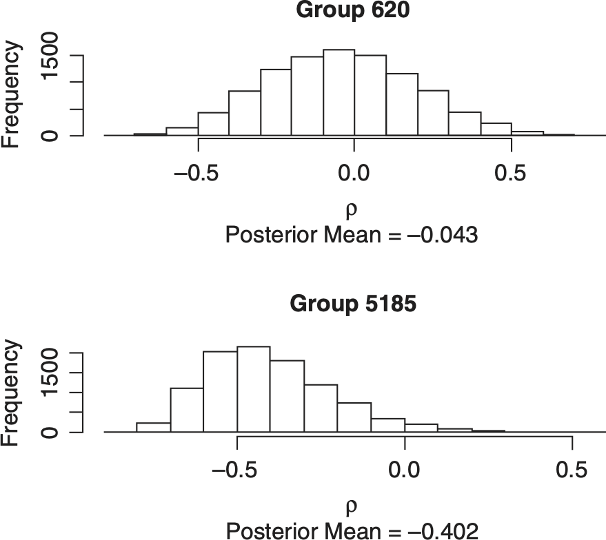
Figure 6.1 gives the standardized residual plots of the SCC model for the illustrative insurers that are analogous to those in Figure 3.2. Figure 6.2 gives the posterior distribution of the ρ parameters for the two-step bivariate SCC model. In Table 6.1 we see that both the PSIS-LOO and the WAIC statistics indicate that the independent bivariate model is the preferred model for Group 620. The two-step bivariate model is the preferred model for Group 5185. The results for all 102 pairs of loss triangles are given in the appendix spreadsheet. For the SCC model, independence is preferred for 95 of the 102 pairs of loss triangles with the PSIS-LOO statistics and for 65 of the 102 pairs for the WAIC statistics. All seven pairs that were favored by the two-step bivariate model with the PSIS-LOO statistic were also favored by the WAIC statistics. Illustrative insurer group 5185 for CA and OL was one of those seven.

Figure 6.1.Standardized residual plots for the SSC model

Figure 6.2.Posterior distribution of $\rho$ for SCC model

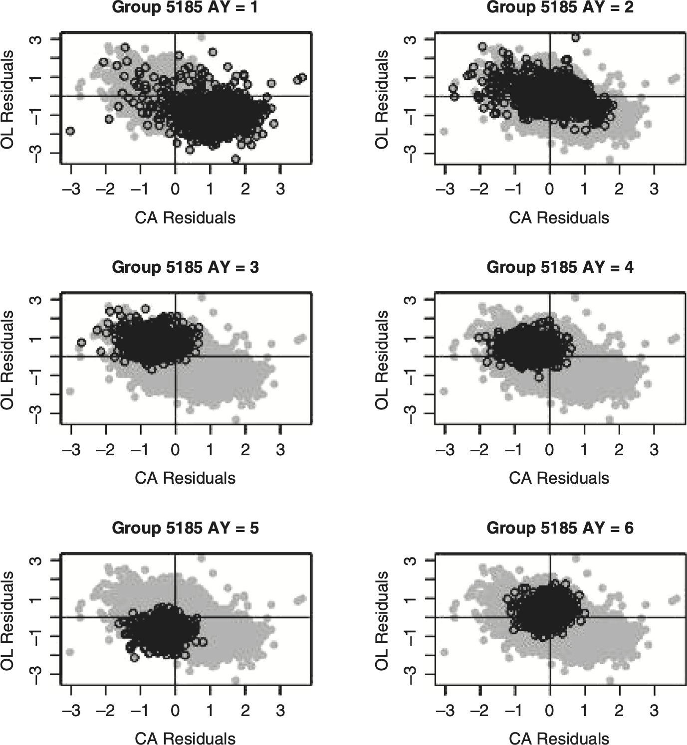
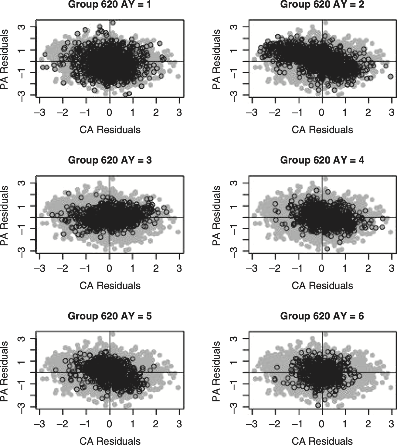
Figures 6.3 and 6.4 explain the underlying cause of the dependency for Group 5185. These figures consist of scatterplots of the standardized residuals for the first six accident years^[7] for the SCC and CSR models. The scatterplots are reproduced six times, with each accident year highlighted. In Figure 6.3 the individual accident year residuals occupy noticeably distinct regions of the scatterplots. The likely cause for these distinct regions are the (either random or systematic) deviations from the assumed constant expected loss ratio assumed in the SCC model. If the regions for the various accident years tend to fall in opposite quadrants (see, for example, accident years 1 and 3 in Figure 6.3) a significant correlation could be indicated. If, as happens with many pairs for the SCC model, the regions are more or less equally spread out in the various quadrants, “independence” will be preferred. By way of contrast, there are no distinct regions by accident year indicated by the CSR model in Figure 6.4.

Figure 6.3.Bivariate standardized residual plots for the SCC model

Figure 6.4.Bivariate standardized residual plots for the CSR model

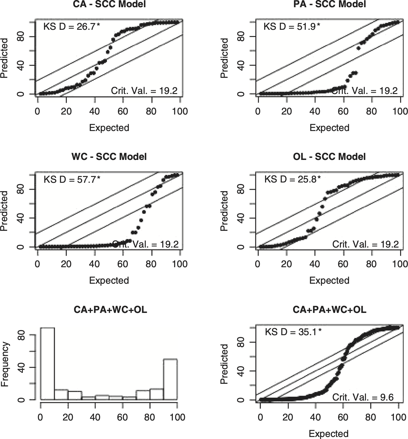
It is also worth noting that, as shown in Figure 6.5, the SCC model fails the uniformity test that the CSR model passed, as shown in Figure 3.1.

Figure 6.5.Uniformity test for the SCC model

Here we see an example where the suboptimal SCC model leads to artificial dependencies between lines, whereas the CSR model leads to independence between lines for our sample of insurer loss triangles.

7. Summary and conclusions

The reason that the dependency problem is so important is that risk-based insurer solvency standards are based on the total risk to the insurance company. Ignoring a true dependency could understate the total risk faced by an insurer. On the other hand, too stringent of a solvency standard could limit the supply of insurance. If this holds, then the current practice in some jurisdictions could limit the supply of insurance.

The purpose of this paper was to illustrate how to build a model that creates a bivariate distribution given two univariate Bayesian MCMC models that preserve the original univariate distributions. While this modeling technique was applied to lognormal stochastic loss reserve models, it should not be difficult to apply this two-step approach to other Bayesian MCMC models using bivariate copulas as was done by Zhang and Dukic (2013).

The conclusion that the within-group pairs of loss triangles are independent for the CSR model may come as a surprise to some. But the evidence supporting this conclusion is as follows.

1. The univariate models did well in two fairly restrictive tests (i.e., the retrospective test in Figure 3.1 and the standardized residual tests in Figure 3.2) that could disqualify many suboptimal models. Thus we should not expect to see an artificial appearance of dependency due to a bad model.

2. The retrospective results of Section 4 indicate support for the independence assumption over the bivariate two-step model.

3. The prospective model selection statistics in Section 5 indicated a preference for the independence assumption for all 102 within-group pairs of lines.

The range of ρs for the 102 within-group pairs contained both positive and negative values, which appear to be random in light of the tests performed in this paper.

While a statistical study such as that done in this paper can never carry the weight of a mathematical proof, its conclusion was derived from the analysis of a large number of within-group pairs of loss triangles. It should be noted that these loss triangles came from NAIC Schedule Ps reported in the same year.

As Bayesian MCMC models become used to set capital requirements, my advice would be test for dependence using the statistics described in this paper. If dependence is indicated, one should try to develop a more refined model.

For now, the CSR model with the independence assumption is looking pretty good. But in light of the high stakes involved, assumptions of this sort need a stringent peer review and replication with new and different data. I look forward to seeing this happen.