1. Introduction
The U.S. Federal Crop Insurance Program (FCIP) started as a federal support program for agriculture in the 1930s. Administered by the U.S. Department of Agriculture (USDA) Risk Management Agency (RMA), the program provides insurance coverage for losses due to various causes. Participation in the program has grown steadily since its inception thanks to legislative changes supporting premium subsidies and the introduction of new insurance products. The aggregate crop coverage level recently reached 74%, according to the Economic Research Service of the USDA.
Figure 1 shows a time series plot of the distribution of commodities covered under the FCIP. The reader may observe that the primary commodity category is the row crops category, whose increase during recent years has been quite dramatic. Figure 2 shows the loss cost ratio (the ratio of losses to premium) over time. Typically a loss cost ratio greater than 1 indicates that the company is losing money from underwriting. In the figure, we see that the loss cost ratio was very high until about the year 2000. Legislative changes mandating crop insurance have contributed to bringing the ratio down in more recent years, as can be seen.

Figure 1.A time series plot of FCIP commodities, 1975–2020
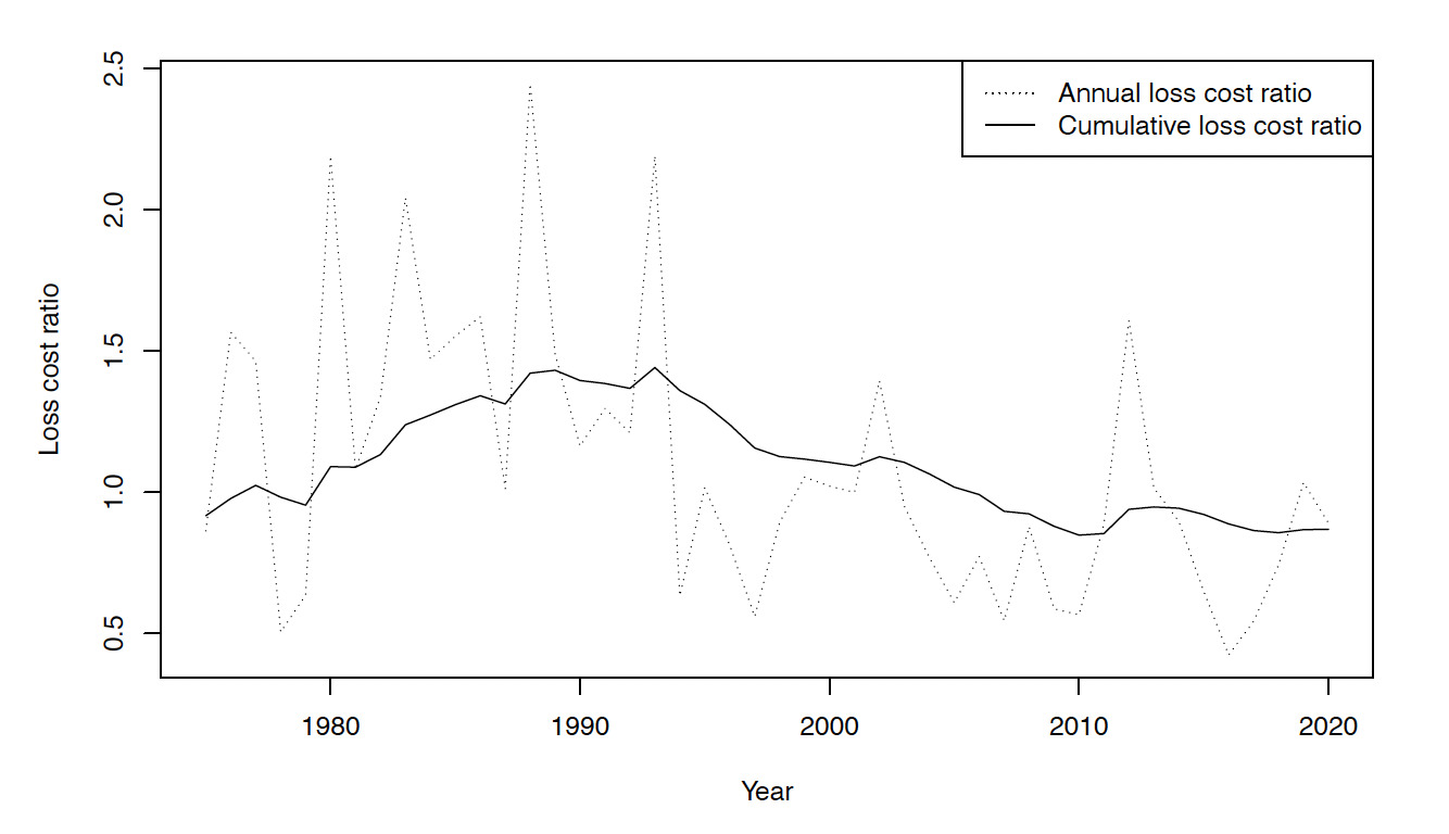
Figure 2.A time series plot of the loss cost ratio, 1975–2020
The program costs of the FCIP are shown in Figure 3. One can see that premium subsidies have increased dramatically in recent years (presumably due to this cost’s correlation with the increase in liability). Premium subsidies have been the primary means of increasing program participation, and the reader may observe that the program does not come without costs. We hope that improvements in the rating engine can help alleviate the costs associated with the crop insurance program and improve its sustainability.

Figure 3.Federal Crop Insurance Program costs, 1975–2020
In actuarial science, we often assume that random variables are defined over positive real numbers. Some examples are the age of a policyholder, the total amount of expenses incurred due to a policy, or the total loss amount from an insured property. Such an assumption simplifies the actuarial theory, and it is a reasonable one to make. For example, we may use distributions that are defined over positive real numbers (take the gamma distribution, for example) to model such variables.
Yet when working with real data, we often discover data that are not consistent with our theories and intuitions. For example, messy real data may contain negative values for a variable that can theoretically only be positive. One example is the company expense variable in National Association of Insurance Commissioners data, where spurious negative values are observed. Another example is the indemnity amount variable in RMA crop insurance data, where negative indemnity amounts can arise when total production amounts are greater than the liability amounts. Formally, the liability amounts in this data set are defined by
Liability=Acres planted×Expected yield (Actual Production History (APH) yield)×Selected coverage level×Base price×Price election percentage,
and the indemnity is defined as
Indemnity=Liability−Value of production, where the value of production is calculated by Value of production=Actual yield×Base price×Price election percentage.
The premium paid is defined by
Premium=Liability× Rate ×Adjustment factor.
Authors such as Shi (2012) and Yu and Zhang (2005) have modeled this type of response using an asymmetric Laplace distribution (ALD) after transforming the response variable. But they faced a problem: the ALD does not have a heavy enough tail to properly model the expense variable. To work around that limitation, the authors relied on transformations of the expense variable.
In this paper, we revisit the illustrated problem and use an alternative approach to solve it. Specifically, we introduce a longer-tailed version of the ALD, which still allows the response to be negative yet fits the data better than the original ALD. Long-tailed modeling of insurance claims has been thoroughly researched in the literature. For example, Sun, Frees, and Rosenberg (2008) studied the properties of a generalized beta 2 (GB2) model to predict nursing home utilization. The GB2 model has since been a popular regression model for long-tailed insurance claims (see Frees and Valdez 2008; Frees, Shi, and Valdez 2009; or Frees, Lee, Lu 2016).
An added feature of our approach is the ability to model data with high-dimensional features. For that reason, the paper is related to the high-dimensional data analysis literature in statistics. In this case, estimation of the regression coefficients becomes a challenging task. The lasso approach to estimating model coefficients with high-dimensional features was introduced into the literature by Tibshirani (1996). The lasso approach basically L1-penalizes the log-likelihood of a regression problem so as to reduce the number of coefficients to be estimated. In the statistics literature, such lasso methods have been applied extensively to linear regression models, generalized linear models, and recently to the Tweedie distribution (see Qian, Yang, and Zou 2016). The Tweedie distribution is useful for modeling the pure premium of insurance losses, where the pure premium is the product of the frequency and severity means of the insurance claims.
Meanwhile, ridge regression—first introduced by Hoerl and Kennard (1970)—is a form of regularized regression, where an L2 penalty term is added to the regression objective function to prevent overfitting and improve the stability of the parameter estimates. Combining the lasso and ridge regression approaches, Zou and Hastie (2005) introduced the elastic net penalty, whereby they proposed a penalized regression approach that combines the L1 and L2 penalties. They demonstrated that the elastic net penalty is particularly effective in handling high-dimensional data with correlated predictors, where either L1 or L2 regularization alone may not perform well.
In this paper, we demonstrate that fast regression routines with elastic net penalties can be built for the modified ALD distribution. Thus the approach would be suitable for situations with a great many explanatory variables, as is the case in the data set used for our empirical study. The high dimensionality of the features results from there being many different categories for the commodity type, unit structure, coverage level percentage, insurance plan type, and coverage type.
The paper proceeds as follows: In Section 2, we summarize the data set used for the empirical analysis so as to give the reader some idea of the problem at hand and the motive for the use of the modified ALD distribution. In Section 3, we explain the details of the modified ALD distribution and the motive behind the distributional form of the model. Section 4 describes the details of the high-dimensional estimation approach for the modified ALD distribution. Section 5 describes a simulation study, where the modified ALD is found to fit longer-tailed data better than the original ALD. In Section 6, we show the results of the estimation. There the reader will discover that the approach with a lasso penalty outperforms the basic model without the lasso penalty. Section 7 concludes the paper.
2. Data description
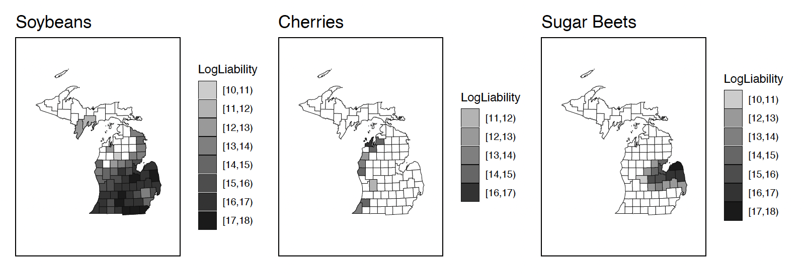
From the state/county/crop summary of business on the USDA RMA website, we use the type/practice/unit structure data files for our analyses. We use 2018 data to form the training sample (in-sample), and 2019 data for the validation sample (out-of-sample). Only Michigan data are used for the purposes of this paper. Within the data set, one may observe that there are different commodities grown at the unit level. As an example, Figure 4 shows the areas in which soybeans, cherries, and sugar beets are grown.

Figure 4.A county-level map of liability amounts for selected commodities
Along with the geographical locations and commodity types, the liability amounts and the indemnity amounts are recorded. A histogram plot of the indemnity amounts appears in the left panel of Figure 5. The right-hand panel of the figure shows a magnified version of the plot for the observations below zero. Here, the reader clearly sees that some of the indemnity values are negative. Note that for the purpose of our analysis, observations with nonzero liability values are taken as a subset, because those with zero liability do not make sense (we believe that only when there is a nonzero liability can there be a meaningful indemnity value).

Figure 5.A plot of the density of the indemnities, and a magnification of the values below zero
Within the state of Michigan data one sees various commodity types, with corn being the most popular, and soybeans the second most. Table 1 summarizes the number of farms, total liability, proportion of nonzero indemnity farms, and average indemnity amounts for each farm in the category. Note that the indemnity severities display significant commodity-level heterogeneity, with apples having the highest average severity.
Table 1.Summary statistics by commodity type
| Commodity |
Num. |
Total |
Prop. |
Avg. |
| farms |
liability (USD) |
nonzero |
indemnity (USD) |
| All other commodities |
237 |
85,518,257 |
0.291 |
42,358 |
| Apples |
253 |
87,336,403 |
0.597 |
135,118 |
| Barley |
14 |
62,766 |
0.500 |
2,903 |
| Blueberries |
45 |
20,787,043 |
0.378 |
31,460 |
| Cabbage |
10 |
1,938,237 |
0.200 |
17,306 |
| Cherries |
93 |
19,069,509 |
0.634 |
46,868 |
| Corn |
1,759 |
714,813,499 |
0.373 |
37,304 |
| Cucumbers |
30 |
8,161,945 |
0.333 |
29,571 |
| Dairy cattle |
41 |
31,600,007 |
0.439 |
25,266 |
| Dry beans |
566 |
78,987,026 |
0.475 |
15,835 |
| Forage production |
66 |
5,935,210 |
0.258 |
8,723 |
| Forage seeding |
3 |
25,180 |
0.000 |
— |
| Grapes |
65 |
10,234,591 |
0.554 |
31,529 |
| Green peas |
1 |
37,252 |
0.000 |
— |
| Hybrid corn seed |
23 |
11,804,251 |
0.130 |
37,421 |
| Oats |
87 |
435,606 |
0.241 |
1,228 |
| Onions |
7 |
1,078,653 |
0.286 |
37,094 |
| Pasture, rangeland, forage |
61 |
1,879,659 |
0.361 |
4,932 |
| Peaches |
44 |
1,070,698 |
0.455 |
5,814 |
| Popcorn |
2 |
316,348 |
1.000 |
61,471 |
| Potatoes |
38 |
28,895,399 |
0.237 |
25,124 |
| Processing beans |
15 |
1,421,824 |
0.067 |
11,900 |
| Soybeans |
1,674 |
605,485,795 |
0.422 |
44,234 |
| Sugar beets |
110 |
78,545,061 |
0.464 |
43,771 |
| Tomatoes |
3 |
1,975,852 |
0.000 |
— |
| Wheat |
884 |
84,886,021 |
0.420 |
12,355 |
| Whole farm revenue protection |
28 |
42,098,170 |
0.464 |
257,995 |
Tables 2, 3, and 4 show that there are observed heterogeneities depending on the unit structure, coverage level percentage, insurance plan categories, and coverage-type code. These features in the data set motivate us to use these categories as rating variables in our regression model for the indemnity amount. The motivation behind a lasso estimation is to reduce overfitting under the presence of many rating variables, and thus ours is precisely the situation under which a lasso estimation technique has advantages.
Table 2.Summary statistics by unit structure
| Unit structure |
Num. |
Total |
Prop. |
Avg. |
| farms |
liability (USD) |
nonzero |
indemnity (USD) |
| Basic unit |
2,359 |
299,825,182 |
0.358 |
17,539 |
| Enterprise unit |
1,461 |
919,499,259 |
0.386 |
57,281 |
| Enterprise unit separated by irrigation practice |
269 |
121,105,160 |
0.301 |
57,892 |
| Optional unit |
2,070 |
583,970,661 |
0.504 |
45,870 |
The coverage level percentage is an interesting variable in the data set. Different coverage levels correspond to different amounts of insurance purchased by the policyholder. Oftentimes, the amount of insurance purchased is used as a variable to detect adverse selection in the insurance market. In these data, the most common coverage percentages were the 50% and 75% levels, each with total liabilities of $314 million and $518 million. The average size of the indemnity was largest in the 50% category, as can be seen in Table 3.
Table 3.Summary statistics by coverage level percentage
| Coverage level |
Num. |
Total |
Prop. |
Avg. |
| percentage |
farms |
liability (USD) |
nonzero |
indemnity (USD) |
| 0% |
62 |
37,913,326 |
0.387 |
24,369 |
| 50% |
1,344 |
314,080,208 |
0.201 |
70,476 |
| 55% |
123 |
7,689,491 |
0.106 |
6,553 |
| 60% |
448 |
41,688,526 |
0.232 |
28,352 |
| 65% |
581 |
43,993,710 |
0.313 |
15,917 |
| 70% |
946 |
203,036,604 |
0.467 |
23,093 |
| 75% |
1,243 |
517,655,825 |
0.553 |
32,347 |
| 80% |
851 |
551,816,613 |
0.592 |
56,604 |
| 85% |
388 |
156,308,197 |
0.601 |
46,152 |
| 90% |
173 |
50,217,762 |
0.422 |
32,868 |
Table 4 shows the insurance plan categories. The most common insurance plan code is RP, which stands for “revenue protection,” where the policy protects the total revenue earned by the policyholder. The next most common is YP, or “yield protection,” where the yield from the commodity is protected instead of the revenue. The revenue protection category alone corresponds to $1.3 billion in total liability, and the yield protection $155 million. Note that the YDO (yield-based dollar amount) category corresponds to the highest average indemnity, and the DO (dollar amount) category the second highest. The insurance plan code exhibit available on RMA’s website defines the other insurance plan codes.
Table 4.Summary statistics by insurance plan
| Insurance |
Num. |
Total |
Prop. |
Avg. |
| plan |
farms |
liability (USD) |
nonzero |
indemnity (USD) |
| APH |
858 |
267,209,831 |
0.418 |
72,195 |
| ARH |
103 |
20,099,655 |
0.660 |
43,983 |
| ARP |
85 |
32,415,944 |
0.494 |
44,674 |
| ARP-HPE |
3 |
61,833 |
0.333 |
482 |
| AYP |
99 |
25,059,109 |
0.111 |
41,112 |
| DO |
42 |
10,907,249 |
0.024 |
195,290 |
| LGM |
56 |
37,537,143 |
0.411 |
25,389 |
| LRP |
6 |
376,183 |
0.167 |
901 |
| RI |
93 |
2,898,554 |
0.366 |
4,425 |
| RP |
3,180 |
1,259,121,275 |
0.501 |
37,243 |
| RPHPE |
107 |
14,466,191 |
0.308 |
10,395 |
| SCO-RP |
57 |
720,723 |
0.228 |
4,415 |
| SCO-RPHPE |
1 |
3,497 |
0.000 |
— |
| SCO-YP |
1 |
1,933 |
0.000 |
— |
| WFRP |
37 |
85,006,140 |
0.486 |
262,369 |
| YDO |
27 |
12,688,078 |
0.148 |
34,514 |
| YP |
1,404 |
155,826,924 |
0.237 |
8,907 |
Table 5.Summary statistics by coverage-type code
| Coverage-type |
Num. |
Total |
Prop. |
Avg. |
| code |
farms |
liability (USD) |
nonzero |
indemnity (USD) |
| A |
5,680 |
1,766,276,215 |
0.433 |
38,601 |
| C |
479 |
158,124,047 |
0.152 |
64,765 |
Table 5 shows summary statistics by coverage-type code. The C category stands for CAT (catastrophic) coverage, while all other policies are categorized as A (standing for buy-up) coverage. We observe that the CAT coverage policies have a lesser amount of total liability but a higher average indemnity.
3. Model
Consider the distribution function
F(y;μ,σ,τ)={τexp[−1−τσlog(1+μ−y1+μ)]y≤01−(1−τ)exp[−τσlog(1+μ+y1+μ)]y>0,
where μ>0, σ>0, and 0<τ<1. The reader may understand this as a modified version of the three-parameter asymmetric Laplace distribution. According to Koenker and Machado (1999), Yu and Moyeed (2001), Shi and Frees (2010), Shi (2012), and Yu and Zhang (2005), the distribution for the three-parameter ALD is given by
FALD(y;μ,σ,τ)={τexp[1−τσ(y−μ)]y≤μ1−(1−τ)exp[−τσ(y−μ)]y>μ.
Comparing equations (1) and (2), we see that the modified distribution in (1) looks somewhat similar to the unmodified version in (2) but differs in that it involves a logarithm; also, equation (2) involves the term y−μ.
The motivation for the new distribution is this: When the ALD is used for a regression analysis of heavily skewed insurance loss data, the fit of the distribution is not as good as one hopes. For that reason, Shi and Frees (2010) and Shi (2012) recommend either rescaling or transforming the response before fitting the distribution. The transformation approach introduces an additional parameter, which needs to be estimated, and the analysis becomes somewhat more complicated. The approach is an elegant workaround, but a practicing actuary may find it desirable to use a simpler model that fits the response directly.
So in this paper, instead of using the transformation approach, we propose the alternative distribution function in equation (1). In the distribution, the logarithmic function handles the skewness in the response variable. Notice that if y=0, then the fraction inside the logarithm becomes 1, making the entire term inside the exponential function zero. The density may be obtained by differentiating equation (1):
f(y;μ,σ,τ)={τ(1−τ)σ(1+μ−y)exp[−1−τσlog(1+μ−y1+μ)]y≤0τ(1−τ)σ(1+μ+y)exp[−τσlog(1+μ+y1+μ)]y>0.
Clearly, the expression in equation (3) is a density, because F(y;μ,σ,τ)→1 as y→∞, and F(y;μ,σ,τ)→0 as y→−∞. Also, the density is continuous at zero by design. Compare this with the original density function of the ALD:
f(y;μ,σ,τ)=τ(1−τ)σexp(−y−μσ[τ−I(y≤μ)]).
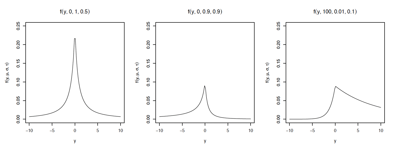
Figure 6 shows the density function for selected parameter values. Notice that for small values of σ and τ, the density becomes highly skewed, allowing for a potentially good fit for heavily skewed insurance loss amounts. The density has the desired property of being defined for (−∞,∞), allowing for negative indemnity amounts.
_for_selected_parameter_values.png)
Figure 6.Plots of the densities in equation (3) for selected parameter values
For regression purposes, we parametrize μ as a linear combination of covariates, with a log link. Specifically, let μ=exp(m), where m=β0+xx′ββ, where β0 and ββ are regression coefficients to be estimated. Also, let σ=exp(s) and τ=exp(t)/(1+exp(t)), with s,t∈(−∞,∞). Then, for a given policyholder i, define
Φi=Φ(yi,β0,ββ,s,t)=−logf(yi;μi,σ,τ),=−logf(yi;exp(β0+xx′iββ),exp(s),exp(t)/(1+exp(t))) where μi=exp(mi)=exp(β0+xx′iββ) for i=1,⋯,n. In order to reduce overfitting by inducing zeros into the coefficients, we seek to find
^θθ=(ˆβ0,^ββT,ˆs,ˆt)T=argminβ0,ββ,s,t[n∑i=1Φi+λp∑j=1(ξwj|βj|+12(1−ξ)β2j)],
where ββ=(β1,⋯,βp)T, λ is a tuning parameter, wj are weights, and ξ defines an elastic net penalty. If ξ=1, then the penalty term reduces to a lasso penalty, but if ξ=0, then the penalty becomes a ridge penalty.
4. Estimation
For the density in equation (3), the explicit form of the contribution Φi of each policy to the negative log-likelihood is given in the appendix. For this specific Φi, it is simple to obtain the form of the gradient and Hessian in terms of the parameter vector θθ, and those derivations are shown in the appendix as well. The estimation is performed iteratively, starting from an initial estimate of the regression coefficients and shape parameters. Assume we have a current estimate ~θθ=(˜β0,~ββ,˜s,˜t) and would like to update it. We take the first-order Taylor’s series approximation around the point ~θθ to the negative log-likelihood:
ℓQ(θθ)=ℓ(~θθ)+n∑i=1(∂˜Φi∂θθ)T(θθ−~θθ)+12n∑i=1(θθ−~θθ)T(∂2˜Φ∂θθ2)(θθ−~θθ).
Then, after some algebra, we can verify that the gradient and Hessian of ℓQ has the following form:
∂ℓQ∂θθ=n∑i=1(∂˜Φi∂θθ)+n∑i=1(∂2˜Φi∂θθ2)(θθ−~θθ).
With this expression, an inner loop is constructed so that the current estimate ˘θθ=(˘β0,˘ββ,˘s,˘t) is updated to ˘θθ(new)=(˘β0,(new),˘ββ(new),˘s(new),˘t(new)) in each iteration. First, we attempt to perform the following for each regression coefficient j within the inner loop:
˘βj,(new)=argminβj[ℓQ(˘θθ)+˘UQ,j(βj−˘βj)+˜γQ,j2(βj−˘βj)2+λ(ξwj|βj|+12(1−ξ)β2j)],
where
˘UQ,j=∂ℓQ∂βj=n∑i=1˘g1xij
and
˜γQ,j=∂2ℓQ∂β2j=n∑i=1˜Φ11x2ij.
The problem in equation (7) is a one-dimensional one, whose first-order condition gives the following:
˘ββj,(new)=(˜γQ,j˘βj−˘UQ,j)(1−λξwj‖˜γQ,j˜βj−˘Uj‖)+˜γQ,j+λ(1−ξ).
The reason the first-order condition gives this update scheme is explained clearly in the lasso literature. The reader is referred to Tibshirani (1996), Yang and Zou (2015), and Qian, Yang, and Zou (2016) for the details. For the intercept and the two shape parameters, we attempt to solve as follows:
\small{
\begin{aligned}
(\breve{\beta}_{0,(new)}, \breve{s}_{(new)}, \breve{t}_{(new)})\\=
\mathop{\mathrm{arg\,min}}_{\beta_0, s, t} & \bigg [
\ell_Q(\breve{\pmb \theta}) + \breve{\pmb U}^T_{Q,shape}
\begin{pmatrix}
\beta_0 - \breve{\beta}_0 \\
s - \breve{s} \\
t - \breve{t}
\end{pmatrix} \nonumber \\
& +
\frac{\tilde{\gamma}_{Q,shape}}{2}
\begin{pmatrix}
\beta_0 - \breve{\beta}_0 \\
s - \breve{s} \\
t - \breve{t}
\end{pmatrix}^T
\begin{pmatrix}
\beta_0 - \breve{\beta}_0 \\
s - \breve{s} \\
t - \breve{t}
\end{pmatrix} \bigg],
\end{aligned} \tag{11}}
where
\breve{U}_{Q, \text { shape }}=\left(\frac{\partial \ell_Q(\breve{\pmb{\theta}})}{\partial \beta_0}, \frac{\partial \ell_Q(\breve{\pmb{\theta}})}{\partial s}, \frac{\partial \ell_Q(\breve{\pmb{\theta}})}{\partial t}\right)^T
\tag{12}
and \tilde{\gamma}_{Q,shape} is the largest eigenvalue of the matrix
\pmb H_{Q,shape}
= \sum_{i=1}^n
\frac{\partial^2 \tilde{\Phi}}{\partial \pmb \theta^2}. \tag{13}
With these, the update for the intercept and the shape parameters is given by
\begin{align}
\begin{pmatrix}
\breve{\beta}_{0,(new)} \\
\breve{s}_{(new)} \\
\breve{t}_{(new)}
\end{pmatrix}&=
\begin{pmatrix}
\breve{\beta}_{0} \\
\breve{s} \\
\breve{t}
\end{pmatrix}\\
&\quad -
\tilde{\gamma}_{Q,shape}^{-1} \breve{\pmb U}_{Q,shape}.
\end{align}
\tag{14}
The reader may wonder why the inverse of the largest eigenvalue is multiplied, instead of the Hessian inverse itself. This approach is called majorization minimization, as explained in Lange, Hunter, and Yang (2000), Hunter and Lange (2004), Wu and Wu and Lange (2010), and Yang and Zou (2015). In a nutshell, the majorization minimization approach is used to construct a stable algorithm, by iteratively minimizing a function that majorizes (is above) the original objective function. Computing the eigenvalues requires time, but nowadays there are fast library routines to perform this task.
This results in algorithm 1. Given a raw design matrix \pmb X^*, in order for the algorithm to run smoothly, one must scale the design matrix using methods described in the appendix so as to obtain \pmb X = (\pmb x_1^T; \pmb x_2^T; \cdots; \pmb x_n^T)^T, where \pmb x_i = (x_{i1}, x_{i2}, \cdots, x_{ip})^T. If there are zero columns in the raw design matrix, then the standard deviation of the entries in those columns is zero (in other words, d_j=0 for that column; see the appendix for details). For those columns, we set x_{ij} = 0 for every i=1,\cdots,n. When running algorithm 1, these zero columns result in zero \tilde{\gamma}_{Q,j} values. So for these columns, we set \beta_j = 0, which is just the initial value for the \beta_j’s.
-
Initialize \tilde{\pmb \theta} and set \breve{\pmb \theta} equal to it.
-
Repeat the following until convergence of \tilde{\pmb \theta}:
-
Repeat the following for j=1, \cdots, p:
-
Compute \tilde{\gamma}_{Q,j} from equation (9).
-
Repeat the following until convergence of \breve{\beta}_j:
-
Compute U_{Q,j} using equation (8).
-
Update \breve{\beta}_j using equation (10).
-
Set \tilde{\beta}_j = \breve{\beta}_j.
-
Compute \tilde{\gamma}_{Q,shape} from equation (13).
-
Repeat the following until convergence of (\breve{\beta}_0, \breve{s}, \breve{t}):
-
Compute \breve{\pmb U}_{Q, shape} using equation (12).
-
Update (\breve{\beta}_0, \breve{s}, \breve{t}) using equation (14).
-
Set \tilde{\pmb \theta} = \breve{\pmb \theta}.
Implementation of this algorithm is a simple but tedious exercise in coding. Writing the routine in R results in a slow algorithm, because of the double looping and the computation of the eigenvalue. For that reason, we recommend using a lower-level language such as Fortran or C++ to implement it. The results we present in Section 6 are obtained using an implementation of algorithm 1 in C++. Nowadays the Rcpp library allows for convenient integration of C++ code into the R environment, so that the routine would be implemented in C++ but could be called from within the R environment.
5. Simulation
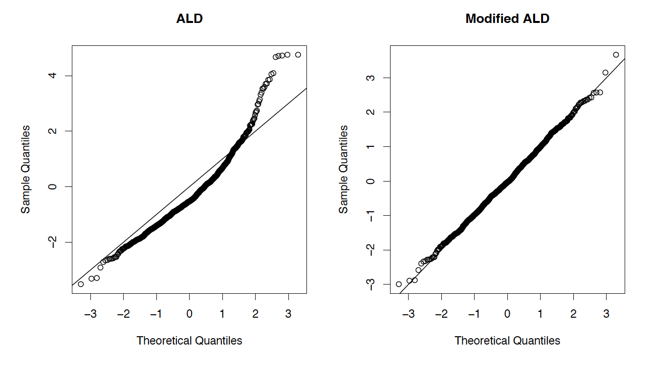
This section describes a simulation study showing that for long-tailed data the modified ALD fits the data better than the original ALD. For the study, synthetic data were generated from a Lomax (Pareto Type II) distribution, with the scale parameter fixed to 10 and the shape parameter varying from 10 down to 2. As the shape parameter decreases, the tail of the data becomes heavier and heavier. Both the ALD and the modified ALD distributions are fit to the data using maximum likelihood estimation (MLE), and the Q–Q plots for the fit are shown. Figure 7 shows the case when the true shape parameter for the data is 10, and Figure 8 shows the case when the shape parameter is 2 (the heavy-tailed case).
.png)
Figure 7.Q–Q plots for the ALD and modified ALD distributions (shape = 10)
.png)
Figure 8.Q–Q plots for the ALD and modified ALD distributions (shape = 2)
From the figures, one can see that the modified ALD fits the data better than the original ALD, especially when the data become heavy-tailed. Although not shown here, we ran the simulation using several other shape parameters, and observed that the fit for the original ALD suffers more and more as the data become more heavy-tailed. This shows precisely when the modified ALD outperforms the original ALD. Note that we have not transformed the data at all, and we are directly modeling the response using the distributions.
As the shape parameter for the Lomax distribution decreased below 1.1 (with it being less than 1 formally called the heavy-tailed case), the original ALD distribution started to give error messages during the estimation using MLE. This indicates that when the data are too heavy-tailed, one cannot use the original ALD distribution without transforming the data.
6. Empirical Results
The model described in Section 3 is estimated using the approach in Section 4 with w_j = 1 for every j=1,\cdots,p and \xi = 0.1 in order to estimate the severity scores. By setting w_j = 1, the same weights are applied to all j’s. We believe this simplifies the analysis, and the results are not influenced much for our purposes. One motive for selecting a small value for \xi as in the paper (\xi = 0.1) could be ease of computation, since the ridge penalty is easier to optimize. In the paper, we made the choice after trial and error, attempting to find a value that seems to generate reasonable predictions. The optimal \lambda is selected by choosing the one that gives the fitted values with the smallest mean squared error (MSE) among a sequence of candidate \lambda’s. In the paper, this value turned out to be \lambda = 101.9. In addition to the regularized indemnity model, a simple logistic regression model is used to predict the indicator of indemnities. The overall indemnity score is obtained by multiplying the predicted indemnity indicator by the severity score predicted by the algorithm.
Because the modified ALD distribution is long-tailed and may not have a finite mean, we cannot rely on the mean for prediction purposes. Instead, we use the lowest MSE quantile as the predictor for the indemnity severities. For this, we need to determine which quantile will give the lowest MSE. To determine that, we rely on the in-sample MSEs and select the quantile that gives the lowest MSE. Then the out-of-sample quantile is obtained.

Figure 9.Prediction results using the modified ALD approach
For comparison, we predict the severity score using a simple MLE regression model (without the lasso penalty) and multiply it to the same predicted indemnity indicator. The indemnity score obtained in this way is called the base model. The out-of-sample correlation with the actual indemnities is taken and compared. The result is shown in Table 6.
Table 6.Spearman correlation with actual indemnities and premiums
|
Base model |
With elastic net |
|
| Correlation with indemnities |
49.19% |
50.57% |
|
| Correlation with premiums |
86.71% |
89.10% |
Table 6 shows that the out-of-sample Spearman correlation improves with the elastic net approach. Thus, we have effectively modeled a response variable with possible negative indemnity values for a ratemaking application, using the modified ALD distribution.
Note that the premiums had a Spearman correlation of 48.63% with the out-of-sample indemnities. This means our ALD approach to modeling the indemnities outperforms the premiums recorded in the RMA data.
7. Conclusion
In this paper, we present a solution to an indemnity modeling problem in the form of a case study using the public RMA data set. The problem we address is that in some data sets, such as the public RMA data set, indemnity amounts may be negative if production levels exceed the liability amounts. The modified ALD distribution gives us an easy way to model the response under such circumstances. In addition, the elastic net approach allows us to incorporate high-dimensional features into our model—the high dimensionality arises because there are many categories for the explanatory variables for the farms.
Compared with other approaches to modeling responses with negative values, the approach introduced here is simple and flexible enough to be used widely in practice. Future work may further analyze the properties of the modified ALD distribution. Application of the modified ALD distribution to the insurance company expense modeling problem may constitute another interesting avenue for future work.
Appendix
Derivation of the gradient and Hessian
The contribution of a policy to the negative log-likelihood used in Section 4 for the density specified in equation (3) is
\scriptsize{\begin{align}
&\Phi =\\
&\begin{cases}
\begin{aligned}
& - \log (\tau) - \log (1 - \tau) + \log(\sigma) + \log(1+\mu-y) + \frac{1-\tau}{\sigma} \log \left( \frac{1+\mu-y}{1+\mu} \right) & y \le 0 \\
& - \log (\tau) - \log (1 - \tau) + \log(\sigma) + \log(1+\mu+y) + \frac{\tau}{\sigma} \log \left( \frac{1+\mu+y}{1+\mu} \right) & y > 0 .
\end{aligned}
\end{cases} \nonumber
\end{align}}
Differentiating this expression with respect to \mu, \sigma, and \tau gives the components of the gradient:
\small{\frac{\partial \Phi}{\partial \mu} =
\begin{cases}
\begin{aligned}
& \displaystyle \frac{1}{1+\mu-y} + \frac{(1-\tau)y}{\sigma(1+\mu)(1+\mu-y)} & y \le 0 \\
& \displaystyle \frac{1}{1+\mu+y} - \frac{\tau y}{\sigma(1+\mu)(1+\mu+y)} & y > 0,
\end{aligned}
\end{cases} \tag{15}}
\small{\frac{\partial \Phi}{\partial \sigma} =
\begin{cases}
\begin{aligned}
& \displaystyle \frac{1}{\sigma} - \frac{1-\tau}{\sigma^2} \log \left( \frac{1+\mu-y}{1+\mu} \right) & y \le 0 \\
& \displaystyle \frac{1}{\sigma} - \frac{\tau}{\sigma^2} \log \left( \frac{1+\mu+y}{1+\mu} \right) & y > 0,
\end{aligned}
\end{cases} \tag{16}}
\small{\frac{\partial \Phi}{\partial \tau} =
\begin{cases}
\begin{aligned}
& \displaystyle - \frac{1}{\tau} + \frac{1}{1-\tau} - \frac{1}{\sigma} \log \left( \frac{1+\mu-y}{1+\mu} \right) & y \le 0 \\
& \displaystyle - \frac{1}{\tau} + \frac{1}{1-\tau} + \frac{1}{\sigma} \log \left( \frac{1+\mu+y}{1+\mu} \right) & y > 0.
\end{aligned}
\end{cases} \tag{17}}
And differentiating these expressions with respect to the parameters once more gives the components of the Hessian matrix:
\scriptsize{\begin{align}
&\frac{\partial^2 \Phi}{\partial \mu^2} =\\
&\begin{cases}
\begin{aligned}
& \displaystyle - \frac{1}{(1+\mu-y)^2} - \frac{(1-\tau)y}{\sigma(1+\mu)^2(1+\mu-y)} \\&\quad- \frac{(1-\tau)y}{\sigma(1+\mu)(1+\mu-y)^2} & y \le 0 \\
& \displaystyle - \frac{1}{(1+\mu+y)^2} + \frac{\tau y}{\sigma(1+\mu)^2(1+\mu+y)} \\&\quad+ \frac{\tau y}{\sigma(1+\mu)(1+\mu+y)^2} & y > 0,
\end{aligned}
\end{cases} \end{align}
\tag{18}}
\small{\frac{\partial^2 \Phi}{\partial \sigma^2} =
\begin{cases}
\begin{aligned}
& \displaystyle - \frac{1}{\sigma^2} + \frac{2(1-\tau)}{\sigma^3} \log \left( \frac{1+\mu-y}{1+\mu} \right) & y \le 0 \\
& \displaystyle - \frac{1}{\sigma^2} + \frac{2 \tau}{\sigma^3} \log \left( \frac{1+\mu+y}{1+\mu} \right) & y > 0,
\end{aligned}
\end{cases} \tag{19}}
\frac{\partial^2 \Phi}{\partial \tau^2}
= \frac{1}{\tau^2} + \frac{1}{(1-\tau)^2}, \tag{20}
\frac{\partial^2 \Phi}{\partial \mu \partial \sigma} =
\begin{cases}
\begin{aligned}
& \displaystyle - \frac{(1-\tau) y }{\sigma^2(1+\mu)(1+\mu-y)} & y \le 0 \\
& \displaystyle \frac{\tau y }{ \sigma^2 (1+\mu) ( 1+\mu+y)} & y > 0,
\end{aligned}
\end{cases} \tag{21}
\frac{\partial^2 \Phi}{\partial \mu \partial \tau}
= - \frac{y}{\sigma(1+\mu)(1+\mu-y)}, \tag{22}
\frac{\partial^2 \Phi}{\partial \sigma \partial \tau} =
\begin{cases}
\begin{aligned}
& \displaystyle \frac{1}{\sigma^2} \log \left( \frac{1+\mu-y}{1+\mu} \right) & y \le 0 \\
& \displaystyle -\frac{1}{\sigma^2} \log \left( \frac{1+\mu+y}{1+\mu} \right) & y > 0.
\end{aligned}
\end{cases} \tag{23}
Given that \mu = \exp(m), \sigma = \exp(s), and \tau = \exp(t) / (1+\exp(t)), we also have
\begin{align}
\frac{\partial \mu}{\partial m} &= \exp(m) = \mu, \\
\quad
\frac{\partial \sigma}{\partial s} &= \exp(s) = \sigma, \\
\quad
\frac{\partial \tau}{\partial t} &= \frac{\exp(t)}{(1+\exp(t))^2} \end{align}
\tag{24}
and
\begin{align}\frac{\partial^2 \mu}{\partial m^2} &= \exp(m) = \mu, \\\quad
\frac{\partial^2 \sigma}{\partial s^2} &= \exp(s) = \sigma, \\\quad
\frac{\partial^2 \tau}{\partial t^2} &= \frac{\exp(t)(1-\exp(t))}{(1+\exp(t))^3}. \end{align}\tag{25}
The gradient and Hessian with respect to \beta_0, \pmb \beta, s, and t can be obtained by the chain rule:
\frac{\partial \Phi}{\partial m} = \frac{\partial \Phi}{\partial \mu} \frac{\partial \mu}{\partial m} = \frac{\partial \Phi}{\partial \mu} \mu, \tag{26}
\frac{\partial \Phi}{\partial s} = \frac{\partial \Phi}{\partial \sigma} \frac{\partial \sigma}{\partial s}
= \frac{\partial \Phi}{\partial \sigma} \sigma, \tag{27}
\frac{\partial \Phi}{\partial t} = \frac{\partial \Phi}{\partial \tau} \frac{\partial \tau}{\partial t}
= \frac{\partial \Phi}{\partial \tau} \frac{\exp(t)(1-\exp(t))}{(1+\exp(t))^3}, \tag{28}
\begin{align}
\frac{\partial^2 \Phi}{\partial m^2} &=
\frac{\partial^2 \Phi}{\partial \mu^2}
\left(\frac{\partial \mu}{\partial m}\right)^2 +
\frac{\partial \Phi}{\partial \mu} \frac{\partial^2 \mu}{\partial m^2}
\\&= \frac{\partial^2 \Phi}{\partial \mu^2} \mu^2 +
\frac{\partial \Phi}{\partial \mu} \mu,
\end{align}
\tag{29}
\begin{align}\frac{\partial^2 \Phi}{\partial s^2} &=
\frac{\partial^2 \Phi}{\partial \sigma^2}
\left(\frac{\partial \sigma}{\partial s}\right)^2 +
\frac{\partial \Phi}{\partial \sigma} \frac{\partial^2 \sigma}{\partial s^2}
\\&= \frac{\partial^2 \Phi}{\partial \sigma^2} \sigma^2 +
\frac{\partial \Phi}{\partial \sigma} \sigma,
\end{align}
\tag{30}
\begin{align}\frac{\partial^2 \Phi}{\partial t^2} &=
\frac{\partial^2 \Phi}{\partial \tau^2}
\left(\frac{\partial \tau}{\partial t}\right)^2 +
\frac{\partial \Phi}{\partial \tau} \frac{\partial^2 \tau}{\partial t^2}
\\&= \frac{\partial^2 \Phi}{\partial \tau^2} \frac{\exp(t)^2}{(1+\exp(t))^4} \\
&\quad +
\frac{\partial \Phi}{\partial \tau} \frac{\exp(t)(1-\exp(t))}{(1+\exp(t))^3},
\end{align}
\tag{31}
\frac{\partial^2 \Phi}{\partial m \partial s} =
\frac{\partial^2 \Phi}{\partial \mu \partial \sigma}
\left(\frac{\partial \mu}{\partial m}\right) \left(\frac{\partial \sigma}{\partial s}\right)
= \frac{\partial^2 \Phi}{\partial \mu \partial \sigma} \mu \sigma, \tag{32}
\begin{align}\frac{\partial^2 \Phi}{\partial m \partial t} &=
\frac{\partial^2 \Phi}{\partial \mu \partial \tau}
\left(\frac{\partial \mu}{\partial m}\right) \left(\frac{\partial \tau}{\partial t}\right)
\\&= \frac{\partial^2 \Phi}{\partial \mu \partial \tau} \mu \ \frac{\exp(t)}{(1+\exp(t))^2}, \end{align}\tag{33}
\begin{align}
\frac{\partial^2 \Phi}{\partial s \partial t} &=
\frac{\partial^2 \Phi}{\partial \sigma \partial \tau}
\left(\frac{\partial \sigma}{\partial s}\right) \left(\frac{\partial \tau}{\partial t}\right) \\
&= \frac{\partial^2 \Phi}{\partial \sigma \partial \tau} \sigma \frac{\exp(t)}{(1+\exp(t))^2}.
\end{align}
\tag{34}
For notational convenience, we define \pmb{h} = (m, s, t)^T, so that
\frac{\partial \Phi}{\partial \pmb h} = (g_1, g_2, g_3)^T = \left( \frac{\partial \Phi}{\partial m}, \frac{\partial \Phi}{\partial s}, \frac{\partial \Phi}{\partial t} \right)^T \tag{35}
and
\begin{align}
\frac{\partial^2 \Phi}{\partial \pmb{h}^2}&=\left[\begin{array}{lll}
\Phi_{11} & \Phi_{12} & \Phi_{13} \\
\Phi_{21} & \Phi_{22} & \Phi_{23} \\
\Phi_{31} & \Phi_{32} & \Phi_{33}
\end{array}\right]\\
&=\left[\begin{array}{ccc}
\frac{\partial^2 \Phi}{\partial m^2} & \frac{\partial^2 \Phi}{\partial m \partial s} & \frac{\partial^2 \Phi}{\partial m \partial t} \\
\frac{\partial^2 \Phi}{\partial s \partial m} & \frac{\partial^2 \Phi}{\partial s^2} & \frac{\partial^2 \Phi}{\partial s \partial t} \\
\frac{\partial^2 \Phi}{\partial t \partial m} & \frac{\partial^2 \Phi}{\partial t \partial s} & \frac{\partial^2 \Phi}{\partial t^2}
\end{array}\right]
\end{align}
\tag{36}
where we assume the subscript i is omitted for succinct notations in all of the expressions above. Also, if we let \pmb \theta = (\beta_0, \pmb \beta^T, s, t)^T, then
\frac{\partial \Phi}{\partial \pmb \theta}
= \left(g_1, g_1 \pmb x^T, g_2, g_3 \right)^T, \tag{37}
\frac{\partial^2 \Phi}{\partial \pmb \theta^2}
= \begin{bmatrix}
\Phi_{11} & \Phi_{11} \pmb x^T & \Phi_{12} & \Phi_{13} \\
\Phi_{11} \pmb x & \Phi_{11} \pmb x\pmb x^T & \Phi_{12} \pmb x & \Phi_{13} \pmb x \\
\Phi_{21} & \Phi_{21} \pmb x^T & \Phi_{22} & \Phi_{23} \\
\Phi_{31} & \Phi_{31} \pmb x^T & \Phi_{32} & \Phi_{33} \\
\end{bmatrix}, \tag{38}
where, again, the subscript i is omitted in all of the terms for the sake of succinct notation.
Details of the scaled design matrix
For all of the analyses in Section 4, the scaled design matrix is used. Let \pmb x^*_{ij} denote the ith row of the jth column of the original, unscaled design matrix. To scale the columns of the design matrix, define
c_j = \frac{1}{n} \sum_{i=1}^n x^*_{ij}, d_j = \sqrt{\frac{1}{n-1} \sum_{i=1}^n \left( x^*_{ij} - c_j \right)^2 }. \tag{39}
The elements of the scaled design matrix are
\begin{align}
x_{ij} &= \frac{x_{ij}^* - c_j}{d_j} \quad \text{for} \quad i=1, \cdots, n \quad \text{and} \\
j&=1, \cdots, p.
\end{align}
\tag{40}
To obtain the coefficients corresponding to the original design matrix, consider
\mu_i = \exp \left( \beta_0 + \sum_{j=1}^p x_{ij} \beta_j \right). \tag{41}
Then define
\beta_0^* = \beta_0 - \sum_{j=1}^p \left( \frac{\beta_j \times c_j}{d_j} \right), \quad \beta_j^* = \frac{\beta_j}{d_j}. \tag{42}
Then we have
\small{\begin{aligned}
\mu_i
& = \exp \left( \beta_0^* + \sum_{j=1}^p x_{ij}^* b_j^* \right) \\
& = \exp \left( \beta_0 - \sum_{j=1}^p \left( \frac{\beta_j \times c_j}{d_j} \right) + \sum_{j=1}^p x_{ij}^* \left( \frac{\beta_j}{d_j} \right) \right) \\
& = \exp \left( \beta_0 - \sum_{j=1}^p \left( \frac{x^*_{ij} - c_j}{d_j} \right) \beta_j \right) \\
& = \exp \left( \beta_0 - \sum_{j=1}^p x_{ij} \beta_j \right).
\end{aligned} \tag{43}}
Thus, once the estimation is performed with the transformed design matrix, the resulting coefficients may be transformed and used with the original designed matrix.
Parameter estimates
Some of the estimated parameters are reported here. It is not practical to report all of them, as there are 285 parameters.
Table A.1.A comparison of the estimated parameters
| Parameter name |
Base model |
Elastic net estimate |
| \beta_0 |
4.165015 |
7.482589 |
| \beta_1 |
0.643526 |
0.643334 |
| \beta_2 |
0.397095 |
0.343269 |
| \beta_3 |
-0.248611- |
-0.316513- |
| ⋮ |
⋮ |
⋮ |
| \sigma |
0.000068 |
0.000183 |
| \tau |
0.041850 |
0.041783 |
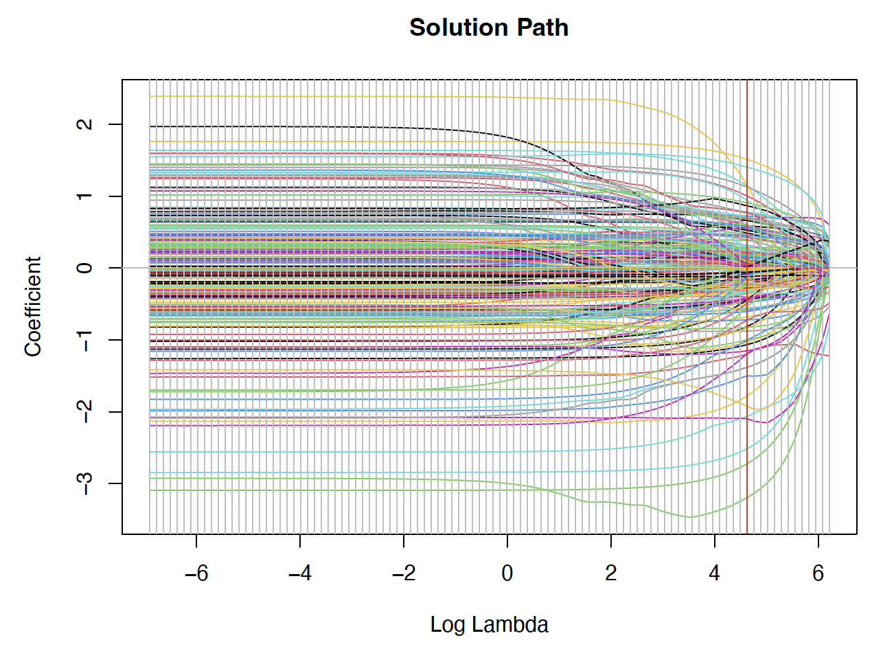
Figure A.1.A plot of the solution paths for the elastic net estimates
Additional summary statistics
Additional summary statistics are provided in Tables A.2, A.3, and A.4.
Table A.2.Summary statistics by county
| County |
Num. |
Total |
Prop. |
Avg. |
County |
Num. |
Total |
Prop. |
Avg. |
| farms |
liability (USD) |
nonzero |
indemnity (USD) |
farms |
liability (USD) |
nonzero |
indemnity (USD) |
| Alcona |
21 |
2,060,153 |
0.524 |
29,524 |
Leelanau |
53 |
14,232,801 |
0.377 |
75,801 |
| All other counties |
237 |
85,518,257 |
0.291 |
42,358 |
Lenawee |
128 |
98,765,037 |
0.289 |
45,347 |
| Allegan |
131 |
43,074,924 |
0.305 |
21,631 |
Livingston |
49 |
13,967,619 |
0.531 |
29,120 |
| Alpena |
33 |
3,294,023 |
0.212 |
10,397 |
Macomb |
55 |
10,187,344 |
0.618 |
15,055 |
| Antrim |
28 |
4,688,181 |
0.286 |
21,118 |
Manistee |
25 |
1,646,811 |
0.640 |
35,311 |
| Arenac |
103 |
18,260,037 |
0.388 |
13,791 |
Mason |
79 |
9,903,979 |
0.342 |
24,739 |
| Barry |
103 |
25,941,132 |
0.252 |
15,615 |
Mecosta |
78 |
9,637,782 |
0.436 |
13,603 |
| Bay |
200 |
59,520,814 |
0.430 |
24,788 |
Menominee |
28 |
4,836,025 |
0.643 |
120,941 |
| Berrien |
192 |
41,981,194 |
0.443 |
47,992 |
Midland |
106 |
16,041,925 |
0.491 |
18,474 |
| Branch |
111 |
49,856,574 |
0.378 |
40,929 |
Missaukee |
32 |
5,709,315 |
0.031 |
21,632 |
| Calhoun |
103 |
58,029,711 |
0.544 |
120,792 |
Monroe |
88 |
59,954,616 |
0.398 |
34,210 |
| Cass |
112 |
32,943,882 |
0.330 |
26,902 |
Montcalm |
192 |
36,133,530 |
0.406 |
21,610 |
| Chippewa |
15 |
83,333 |
0.600 |
3,986 |
Muskegon |
79 |
17,695,798 |
0.468 |
106,666 |
| Clare |
46 |
2,404,059 |
0.283 |
12,762 |
Newaygo |
89 |
21,961,382 |
0.416 |
25,671 |
| Clinton |
143 |
48,056,028 |
0.371 |
47,911 |
Oakland |
17 |
2,190,325 |
0.529 |
31,103 |
| Delta |
30 |
1,092,939 |
0.633 |
20,175 |
Oceana |
87 |
18,028,949 |
0.460 |
80,991 |
| Eaton |
109 |
47,959,482 |
0.450 |
34,365 |
Ogemaw |
40 |
5,798,201 |
0.400 |
17,005 |
| Genesee |
81 |
20,732,922 |
0.420 |
31,758 |
Osceola |
42 |
3,400,197 |
0.238 |
4,510 |
| Gladwin |
45 |
4,047,067 |
0.356 |
26,407 |
Ottawa |
135 |
44,923,865 |
0.385 |
52,137 |
| Grand Traverse |
61 |
9,012,722 |
0.344 |
15,748 |
Presque Isle |
57 |
3,160,427 |
0.193 |
11,928 |
| Gratiot |
227 |
74,328,762 |
0.467 |
26,087 |
Saginaw |
226 |
84,369,548 |
0.403 |
23,768 |
| Hillsdale |
91 |
49,116,046 |
0.407 |
44,952 |
Sanilac |
248 |
99,155,849 |
0.367 |
24,047 |
| Huron |
287 |
124,444,777 |
0.376 |
22,486 |
Shiawassee |
124 |
51,096,460 |
0.500 |
41,123 |
| Ingham |
72 |
40,912,817 |
0.653 |
42,830 |
St. Clair |
104 |
23,552,161 |
0.587 |
24,811 |
| Ionia |
142 |
48,773,769 |
0.394 |
31,718 |
St. Joseph |
127 |
27,638,794 |
0.354 |
11,463 |
| Iosco |
27 |
2,748,607 |
0.370 |
14,604 |
Tuscola |
297 |
94,352,927 |
0.404 |
22,069 |
| Isabella |
163 |
30,959,151 |
0.479 |
28,241 |
Van Buren |
141 |
53,277,996 |
0.546 |
89,458 |
| Jackson |
73 |
35,466,587 |
0.575 |
92,912 |
Washtenaw |
88 |
32,220,349 |
0.466 |
73,181 |
| Kalamazoo |
78 |
21,392,626 |
0.410 |
20,535 |
Wayne |
23 |
1,559,426 |
0.565 |
33,530 |
| Kent |
122 |
47,307,469 |
0.475 |
134,877 |
Wexford |
16 |
1,125,879 |
0.063 |
1,679 |
| Lapeer |
120 |
23,866,900 |
0.383 |
21,432 |
|
|
|
|
|
Table A.3.Summary statistics by type
| Type |
Num. |
Total |
Prop. |
Avg. |
| farms |
liability (USD) |
nonzero |
indemnity (USD) |
| Adzuki |
19 |
702,567 |
0.579 |
10,549 |
| Alfalfa |
54 |
5,961,304 |
0.241 |
10,604 |
| Alfalfa grass mixture |
16 |
291,914 |
0.125 |
720 |
| All other food grades |
20 |
770,018 |
0.300 |
5,249 |
| Annuals |
1 |
32 |
0.000 |
— |
| Birdsfoot trefoil |
1 |
7,941 |
0.000 |
— |
| Birdsfoot trefoil grass mixture |
2 |
35,536 |
1.000 |
4,499 |
| Black |
285 |
42,803,911 |
0.516 |
17,581 |
| Blue |
12 |
893,226 |
0.750 |
12,599 |
| Broadleaf evergreen shrubs |
4 |
635,165 |
0.000 |
— |
| Broadleaf evergreen trees |
2 |
13,850 |
0.000 |
— |
| Calendar year filer |
33 |
80,608,659 |
0.485 |
284,348 |
| Commodity |
1,525 |
592,910,171 |
0.428 |
46,800 |
| Coniferous evergreen shrubs |
4 |
172,862 |
0.000 |
— |
| Coniferous evergreen trees |
4 |
5,649,266 |
0.000 |
— |
| Cranberry |
18 |
1,146,195 |
0.444 |
6,798 |
| Dairy weight 2 |
1 |
68,224 |
0.000 |
— |
| Dark red kidney |
12 |
361,285 |
0.250 |
14,724 |
| Deciduous shrubs |
4 |
1,588,071 |
0.000 |
— |
| Deciduous trees (shade, flower) |
4 |
416,073 |
0.000 |
— |
| Early fiscal year filer |
3 |
3,995,597 |
0.667 |
86,535 |
| Farrow to finish |
9 |
1,748,272 |
0.222 |
5,255 |
| Foliage |
2 |
5,522 |
0.000 |
— |
| Fresh |
122 |
31,688,418 |
0.574 |
130,834 |
| Fruit and nut trees |
3 |
1,818,215 |
0.333 |
195,290 |
| Grain |
1,730 |
712,693,685 |
0.375 |
37,732 |
| Grazing |
13 |
51,238 |
0.615 |
261 |
| Great northern |
5 |
209,415 |
0.600 |
8,880 |
| Green (fresh) |
11 |
4,647,964 |
0.273 |
8,057 |
| Ground cover and vines |
2 |
67,415 |
0.000 |
— |
| Group A |
32 |
6,317,864 |
0.719 |
29,270 |
| Group B |
10 |
1,096,879 |
0.300 |
7,189 |
| Haying |
80 |
2,847,316 |
0.325 |
5,706 |
| Heifers weight 1 |
1 |
18,160 |
0.000 |
— |
| Heifers weight 2 |
1 |
16,209 |
0.000 |
— |
| Herbaceous perennials |
2 |
194,466 |
0.000 |
— |
| High protein |
9 |
489,489 |
0.556 |
10,070 |
| Highbush |
46 |
20,800,402 |
0.391 |
30,059 |
| Interplanting |
4 |
638,747 |
0.000 |
— |
| Large seeded food grade |
100 |
10,549,984 |
0.410 |
14,577 |
| Late fiscal year filer |
1 |
401,884 |
0.000 |
— |
| Late season |
1 |
37,252 |
0.000 |
— |
| Light red kidney |
28 |
2,012,575 |
0.429 |
8,754 |
| Liners |
2 |
101,175 |
0.000 |
— |
| Low linolenic acid |
7 |
587,702 |
0.286 |
16,745 |
| Low saturated fat |
9 |
383,285 |
0.000 |
— |
| Native spearmint |
2 |
1,899,068 |
0.500 |
144,838 |
| Niagara |
23 |
2,819,848 |
0.435 |
44,028 |
| No type specified |
265 |
118,765,929 |
0.362 |
30,778 |
| Oil |
1 |
26,089 |
1.000 |
15,499 |
| Pea (navy) |
140 |
29,678,866 |
0.464 |
17,960 |
| Peppermint |
1 |
5,544 |
0.000 |
— |
| Pickling |
39 |
9,577,028 |
0.282 |
27,254 |
| Pink |
1 |
372 |
0.000 |
— |
| Pinto |
26 |
665,779 |
0.577 |
6,608 |
| Processing |
72 |
9,058,784 |
0.583 |
31,250 |
| Red (fresh) |
11 |
987,734 |
0.455 |
10,930 |
| Reds |
4 |
106,582 |
0.000 |
— |
| Reds non-seed |
5 |
65,742 |
0.200 |
945 |
| Reds seed |
1 |
2,425 |
1.000 |
1,533 |
| Roses |
3 |
74,093 |
0.000 |
— |
| Russets non-seed |
14 |
2,468,561 |
0.071 |
3,589 |
| Russets seed |
2 |
45,678 |
0.000 |
— |
| Seed |
3 |
126,493 |
0.667 |
12,004 |
| Silage |
29 |
2,743,766 |
0.103 |
18,588 |
| Small fruits |
1 |
140,707 |
0.000 |
— |
| Small red |
26 |
1,411,763 |
0.269 |
14,459 |
| Small seeded food grade |
7 |
227,544 |
0.000 |
— |
| Snap |
20 |
1,883,671 |
0.150 |
27,800 |
| Spring |
18 |
167,671 |
0.500 |
5,136 |
| Standard planting |
23 |
12,049,331 |
0.174 |
34,514 |
| Steers & heifers |
1 |
158,696 |
1.000 |
901 |
| Steers weight 1 |
1 |
41,166 |
0.000 |
— |
| Steers weight 2 |
1 |
73,728 |
0.000 |
— |
| Sweet cherries (fresh) |
3 |
182,150 |
0.667 |
8,435 |
| Sweet cherries (processing) |
33 |
4,086,467 |
0.576 |
20,066 |
| Tart cherries (processing) |
67 |
15,831,038 |
0.701 |
55,165 |
| Tebo |
2 |
35,970 |
0.000 |
— |
| Varietal group A (fresh) |
44 |
16,619,592 |
0.545 |
131,162 |
| Varietal group B (fresh) |
39 |
22,064,749 |
0.590 |
177,786 |
| Varietal group C (fresh) |
38 |
11,315,883 |
0.553 |
150,557 |
| White kidney |
6 |
336,175 |
0.000 |
— |
| Whites non-seed |
28 |
33,483,864 |
0.250 |
39,774 |
| Whites seed |
3 |
426,892 |
0.000 |
— |
| Winter |
894 |
85,142,649 |
0.417 |
12,298 |
| Yelloweye |
1 |
315 |
0.000 |
— |
| Yellows |
7 |
1,146,460 |
0.286 |
37,094 |
Table A.4.Summary statistics by practice name
| Practice name |
Num. |
Total |
Prop. |
Avg. |
| farms |
liability (USD) |
nonzero |
indemnity |
| April–May index interval (non-irrigated) |
6 |
162,882 |
0.000 |
— |
| April–Feb. insurance period |
3 |
4,129,120 |
0.333 |
39,320 |
| April–Sept. insurance period |
1 |
134,565 |
0.000 |
— |
| Aug.–Sept. index interval |
2 |
856 |
1.000 |
263 |
| Aug.–Sept. index interval (non-irrigated) |
7 |
135,299 |
1.000 |
9,089 |
| Aug.–Jan. insurance period |
1 |
114,997 |
1.000 |
9,960 |
| Aug.–Jun. insurance period |
7 |
4,614,500 |
0.000 |
— |
| Container |
26 |
3,859,875 |
0.000 |
— |
| Dec.–May insurance period |
1 |
125,391 |
0.000 |
— |
| Dec.–Oct. insurance period |
3 |
1,905,232 |
0.333 |
575 |
| Fac (irrigated) |
2 |
140,043 |
0.500 |
11,900 |
| Feb.–Mar index interval (irrigated) |
1 |
12,228 |
0.000 |
— |
| Feb.–Mar index interval (non-irrigated) |
5 |
268,665 |
0.000 |
— |
| Feb.–Dec. insurance period |
4 |
3,899,065 |
1.000 |
30,610 |
| Feb.–July insurance period |
1 |
237,437 |
0.000 |
— |
| Field grown |
12 |
7,017,037 |
0.083 |
195,290 |
| Irrigated |
671 |
175,738,809 |
0.237 |
43,865 |
| Irrigated with cover crop |
8 |
648,139 |
0.125 |
50,888 |
| Jan.–Feb index interval |
1 |
7,964 |
0.000 |
— |
| Jan.–Feb index interval (non-irrigated) |
4 |
75,740 |
0.000 |
— |
| Jan.–June insurance period |
1 |
502,549 |
0.000 |
— |
| Jan.–Nov. insurance period |
6 |
4,971,203 |
1.000 |
26,240 |
| July–Aug. index interval |
1 |
1,244 |
1.000 |
36 |
| July–Aug. index interval (irrigated) |
2 |
14,416 |
0.500 |
3,042 |
| July–Aug. index interval (non-irrigated) |
9 |
421,580 |
0.556 |
3,032 |
| July–May insurance period |
3 |
2,231,550 |
0.333 |
98,992 |
| July–Dec. insurance period |
1 |
156,479 |
1.000 |
550 |
| June–July index interval |
2 |
14,074 |
1.000 |
678 |
| June–July index interval (irrigated) |
1 |
14,033 |
1.000 |
4,350 |
| June–July index interval (non-irrigated) |
11 |
690,808 |
0.455 |
10,667 |
| June–April insurance period |
4 |
2,674,084 |
0.500 |
23,498 |
| March–April index interval |
3 |
14,132 |
0.000 |
— |
| March–April index interval (irrigated) |
2 |
16,221 |
0.000 |
— |
| March–April index interval (non-irrigated) |
10 |
569,427 |
0.000 |
— |
| March–Aug. insurance period |
1 |
168,706 |
0.000 |
— |
| March–Jan. insurance period |
6 |
3,255,100 |
0.500 |
17,520 |
| May–June index interval |
2 |
3,537 |
1.000 |
31 |
| May–June index interval (irrigated) |
1 |
3,829 |
0.000 |
— |
| May–June index interval (non-irrigated) |
10 |
206,188 |
0.400 |
458 |
| May–March insurance period |
1 |
588,620 |
1.000 |
43,880 |
| Nfac (irrigated) |
321 |
40,905,372 |
0.206 |
12,931 |
| Nfac (irrigated)(OC) |
6 |
113,460 |
0.167 |
8,589 |
| Nfac (irrigated)(OT) |
2 |
40,020 |
0.000 |
— |
| Nfac (non-irrigated) |
1,254 |
560,607,686 |
0.475 |
50,201 |
| Nfac (non-irrigated)(OC) |
78 |
5,367,244 |
0.449 |
14,793 |
| Nfac (non-irrigated)(OT) |
34 |
628,039 |
0.324 |
4,129 |
| No practice specified |
215 |
174,071,366 |
0.488 |
77,011 |
| No practice specified (OC) |
3 |
90,609 |
0.333 |
4,768 |
| Non-irrigated |
3,036 |
873,402,863 |
0.442 |
36,685 |
| Non-irrigated with cover crop |
6 |
847,269 |
0.167 |
23,299 |
| Nov.–Dec. index interval |
1 |
7,964 |
1.000 |
112 |
| Nov.–Dec. index interval (non-irrigated) |
2 |
46,948 |
0.500 |
3,240 |
| Nov.–April insurance period |
1 |
87,465 |
0.000 |
— |
| Nov.–Sept. insurance period |
3 |
877,800 |
0.000 |
— |
| Oct.–Nov. index interval (non-irrigated) |
2 |
20,683 |
0.000 |
— |
| Oct.–Aug. insurance period |
3 |
913,497 |
0.000 |
— |
| Oct.–March insurance period |
1 |
220,683 |
0.000 |
— |
| Organic (certified) irrigated |
16 |
1,298,332 |
0.125 |
23,323 |
| Organic (certified) non-irrigated |
186 |
19,180,114 |
0.581 |
22,373 |
| Organic (transitional) irrigated |
4 |
108,268 |
0.250 |
50,224 |
| Organic (transitional) non-irrigated |
59 |
1,548,466 |
0.441 |
5,278 |
| Sept.–Oct. index interval |
1 |
1,467 |
0.000 |
— |
| Sept.–Oct. index interval (irrigated) |
1 |
2,735 |
0.000 |
— |
| Sept.–Oct. index interval (non-irrigated) |
6 |
185,634 |
0.333 |
1,894 |
| Sept.–July insurance period |
4 |
5,729,100 |
0.500 |
5,625 |
| Spring planted |
12 |
3,184,881 |
0.333 |
11,483 |
| Spring planted irrigated |
11 |
1,203,514 |
0.091 |
4,084 |
| Spring planted non-irrigated |
27 |
8,133,797 |
0.370 |
29,571 |
| Spring seeded (non-irrigated) |
4 |
30,337 |
0.000 |
— |
| Summer planted |
10 |
2,450,817 |
0.400 |
8,223 |
| Summer planted irrigated |
1 |
239,717 |
0.000 |
— |
| Transplanted for hand harvest |
1 |
56,817 |
0.000 |
— |
| Transplanted machine harvest |
5 |
3,051,674 |
0.000 |
— |