Parameter Reduction in Actuarial Triangle Models

undefined

1. Introduction

Triangle models are familiar to casualty actuaries, but statisticians and actuaries who do mortality projections often use similar models. Mortality projection is key these days for annuity calculations, including workers compensation permanent injury claims, which are a form of variable annuity.

Both sets of models start with “triangle” arrays, and both track year of origin (or decade, quarter, etc.). For claims, the year of origin could be policy year, accident year, or report year. For mortality, it is year of birth. The columns in both cases represent the lag from origin to observation. For claims, the observation could be a payment or a reserve change. For mortality, it is demise, so the lag is age at death. The time of observation is the sum of the origin time and the lag. Typically in mortality models, the rows are years of observation, so origin years are northwest-southeast diagonals, while in claims triangles, the rows are years of origin, so the observation times are southwest-northeast diagonals. For simplicity, we will refer to the origin periods as AYs, lags as DYs, and observation times as CYs.

The basic modeling framework reviewed here starts with the probabilistic trend family (PTF), described by Barnett and Zehnwirth (2000). The Renshaw-Haberman (2006) model used in mortality studies generalizes this framework by multiplying (in log form, where the model is a sum) the AY and CY components by the DY factors. We look at a slight generalization of both models that we call the extended PTF (EPTF).

Both the LASSO (least absolute shrinkage and selection operator) and random effects models shrink (i.e., credibility weight) parameters toward 0—often to the point that they are virtually 0. All model selection has some judgment elements built in, and these do as well, although once set up they follow mechanized rules. In addition, the modeling needs to be done in such a way that shrinking toward 0 makes sense. This is often accomplished by taking the parameters as differences from the mean and then, in effect, credibility weighting those toward 0. An example might be color-of-car offsets to loss severity. What we do here is shrink the changes in trend for the three dimensions of time in the triangle parameters, so if some go to 0, that just means the trend continues as it was at those points.

The paper is organized as follows. Section 2 discusses the PTF and shows how to set it up as a regression. Section 3 introduces random effects. Section 4 illustrates the use of random effects on PTF models for loss triangles, and Section 5 looks at EPTF for a mortality example. Section 6 reviews LASSO and illustrates its use. Section 7 concludes the basic analysis. Appendix 1 addresses using parameter reduction on the increasingly popular topic of simultaneous estimation of related triangles. Appendix 2 tries EPTF on a loss triangle.

2. Extended probabilistic trend family

Say you start with the model of y_wd = log of paid losses for origin year w for lag d, indexed to start at w = d = 0:

$$y_{w d}=p_{w}+q_{d}+r_{w+d}+\varepsilon_{w d} .$$

Here p, q, and r are the AY, DY, and CY effects, respectively; q and r are often expressed as sums of trends a and c:

$$q_{d}=\sum_{k=0}^{d} a_{k} ; r_{w+d}=\sum_{k=0}^{w+d} c_{k} .$$

This is what Barnett and Zehnwirth (2000) call the PTF. It can be put into the form y = Xβ + ε. In this notation, y is the entire triangle strung out into a column of length n; X is a design matrix showing, for each observation, to which row, column, and diagonal it belongs; and β is the vector of parameters. If the variables are levels (p, q, r), there is a column of the design matrix for each row, column, and diagonal of the triangle, with indicators 0 or 1 for each observation indicating whether or not the observation comes from that row, column, or diagonal. But if the variables are the trends (a, c), then the a_k parameter is included in all the subsequent periods.

The latter case can be handled by making the variable 1 for k and all later periods. When we make the parameters the changes in trend, then the changes are added to all future trends and thus accumulate like a sequence—1, 2, 3, . . . —across the periods, so that the random variable starts at 1 at the time of the change and then is 2, 3, 4, . . . in the subsequent periods.

To forecast to the end of the triangle, the p and q parameters are already known, but new values of r are needed. Continuing the latest trend is one possibility. Fitting a first-order autoregression process to the trend history is another technique that actuaries use. Sometimes also the CY parameters just pick up some historical high or low diagonals, and no CY projection is done. This method has value in preventing distortions on the AY and DY parameters. If in fact the payment trend is constant, the CY trend is not needed because the AY and DY parameters pick up the trend, but usually trends do change to some degree over time. In any case, good actuarial judgment is an element of the projection task. Here we focus only on the estimation issues.

Two possible extensions of the PTF are as follows:

• It is becoming fairly common for the payout pattern of losses to change, either due to changing technology within the claims department or a change in the mix of losses. One way to handle such a change is to add a mixture effect, g_wh_d, for accident (origin) year (AY) combined with development year (lag, or DY). For instance, Meyers (2015) finds that incorporating a mixture for payout changes provides a better fit to a number of triangles. He attributes this finding to speedier claims handling due to computerized systems. But workers comp is seeing the opposite effect, a slower payout pattern due to a shift away from the less serious injuries that pay faster.

• Calendar-year effects are sometimes stronger for some development years and weaker for others. This variability could be treated by multiplying the trend by a development-year scale, so r_w+d becomes f_dr_w+d. For instance, in workers comp, the early payments are more indemnity weighted, whereas medical picks up later. Wage levels are more of an accident-year effect, so the calendar-year trend from medical might be stronger later on. Also, the very end of the triangle often sees a noisier payout pattern, which could show less impact of the CY trend.

The EPTF is not a linear model, as parameters are multiplied with each other. It can be written as follows:

$$y_{w d}=p_{w}+q_{d}+f_{d} r_{w+d}+g_{w} h_{d}+\varepsilon_{w d} .$$

In addition, f, g, and h can be expressed as sums of trends:

$$\begin{array}{c} q_{d}=\sum_{k=0}^{d} a_{k} \ldots ; r_{w+d}=\sum_{k=0}^{w+d} c_{k} \ldots ; f_{d}=\sum_{k=0}^{d} l_{k} \ldots ; \\ g_{w}=\sum_{k=0}^{w} m_{k} \ldots ; h_{d}=\sum_{k=0}^{d} t_{k} \end{array}$$

Models like these are often estimated sequentially by regarding some of the parameters as constants and estimating the others, and then reversing the roles. In this case, the DY parameters could be taken as constants, for instance, and all the others estimated, then those taken as constants at those values and the DYs estimated, iteratively, until they all converge.

This model is also an extension of the Renshaw-Haberman (2006) model used in mortality trend modeling. In fact, setting p_w to 0 gives that model. However, the EPTF may work there as well—it would just generalize the cohort effect slightly. For both losses and mortality trends, the extra parameters would not be included unless they are necessary, in which case they are treated as random effects. In addition, we will treat the changes in trend as random effects.

3. Random effects

Random effects can be added to the regression models to give linear mixed models (LMMs),^[1] as follows:

$$y=X \beta+Z b+\varepsilon,$$

where

• y is the n-by-1 response vector, and n is the number of observations,

• X is the usual n-by-p fixed-effects design matrix,

• β is a p-by-1 fixed-effects parameter vector,

• Z is an n-by-q random-effects design matrix,

• b is a q-by-1 random-effects parameter vector, and

• ε is the n-by-1 observation error vector.

The random-effects vector, b, and the error vector, ε, are assumed to have the following independent distributions:

$$b \sim N\left[0, \sigma^{2} D(\theta)\right], \varepsilon \sim N\left[0, \sigma^{2} I\right],$$

where D is a symmetric and positive semidefinite matrix, parameterized by a variance component vector θ; I is an n-by-n identity matrix; and σ² is the error variance.

In this model, the parameters to estimate are the fixed-effects coefficients, β, and the variance components, θ and ε. The error distribution here is normal, but a generalized LMM simply exponentiates the mean and uses any distribution in the exponential family for the residuals. Most software programs provide that option. If you concatenate X and Z, you get an n-by-p+q design matrix for the concatenation of β and b as the parameters, so this model effectively divides the design matrix variables into two sets, only one of whose parameters get shrunk.

Often but not always, D(θ) is taken as diagonal with a variance for each parameter, which is estimated along with b, making the random effects independent. We will assume that case here. The fact that one unbiased estimate of each random effect is 0 and another could come from standard regression sets up a credibility weighting that shrinks such parameters toward 0.

A random-effect parameter is shrunk more toward 0 if its variance from D is low and its variance from parameter error is high. This is a lot like standard least-squares credibility, except that each parameter has its own variance from 0 that is estimated by maximum likelihood estimation (MLE), whereas in credibility theory, the parameters are distributed around their mean with a constant variance. For a more detailed discussion of random effects and credibility, see Klinker (2011).

MLE in this case maximizes the joint likelihood of P(y, b) = P(y|b)P(b), showing that there are opposite pulls on b in the joint likelihood function. P(b) has a maximum at b = 0, since it is just a normal density. But P(y|b) has its maximum at the value of b estimated as a fixed effect. Since the product of these factors has to be maximized, the estimate will end up somewhere between 0 and the fixed-effects value. By the definition of conditional probability, we also have P(y, b) = P(b|y)P(y). Here we can regard P(y) as a constant, so maximizing the joint likelihood also maximizes the probability of the random-effect parameters given the data.

The variance of each random effect is also estimated and has a similar pull. The larger that variance is, the lower is the P(b) probability at 0, but the shrinkage toward 0 is less, so the estimate is closer to its fixed-effects value, which increases the P(y|b) factor. The random effects that are pulled less toward 0 are thus the ones that make more of an improvement in the P(y|b) term. The joint log-likelihood is as follows:

$$\begin{aligned} \log L\left(\beta, \theta, b, \sigma^{2}\right)= & -\frac{n}{2} \log \left(\sigma^{2}\right)-\frac{S S R}{2 \sigma^{2}} \\ & -\frac{1}{2} \sum_{i=1}^{q}\left[\log \sigma^{2}+\log \theta_{i}+\frac{b_{i}^{2}}{\sigma^{2} \theta_{i}}\right] \\ & -\frac{n+q}{2} \log 2 \pi \end{aligned}$$

For the estimation, first note that given D, the variance of y is known to be σ²(ZDZ′ + I) = σ²V. Then, given D and σ², log L is minimized at

$$\hat{\beta}=\left(X^{\prime} V^{-1} X\right)^{-1} X^{\prime} V^{-1} y$$

$$\hat{b}=D Z^{\prime} V^{-1}(y-X \hat{\beta}) .$$

Let SSR be the sum of the ε squared. Then the likelihood can be maximized for σ² and θi by the following:

$$\sigma^{2}=\frac{S S R}{n}$$

and

$$\theta_{i}=\frac{b_{i}^{2}}{\sigma^{2}} .$$

For a mean-0 normal, the probability at b is maximized with variance b, so the likelihood for each b is maximized at this value of θ_i. With these variance estimates, the regression coefficients and then the variances can be reestimated, alternating iteratively. That is, we can start with judgment estimates of σ² and θ_i, use those to estimate the b and β parameters, and then reestimate σ² and θ_i, and so on.

This is a form of fixed-point iteration and seems to work well for this model. However, fitting packages such as SAS and MATLAB use more complex approaches because they are set up to solve more general models. All of the estimation methods appear to end up with slightly different fits of the model, possibly with a few different parameters going to 0. When estimating EPTF for large data sets, fixed-point iteration is often much faster—about 250 times faster than MATLAB in one such case.

Once a method converges to MLE estimates, the information matrix (all mixed second derivatives of the negative log-likelihood) can be computed in a straightforward, if tedious, way, or estimated numerically, to get the parameter error distributions. It is usually easier to get the derivatives with respect to the fixed- and random-effect means, and then use the chain rule on those to get the derivatives with respect to the parameters.

The hat matrix in linear models is used to calculate estimated values of each observation from observed values: ŷ = Hy. Since the parameters are estimated as β̂ = (X′X)^–1X′y, and the fitted values of y are given by ŷ = Xβ̂, then ŷ = (X′X)^–1 X′y, and so H = X(X′X)^–1 X′. The diagonal of the hat matrix thus shows how much an observation affects its estimate and is therefore the derivative of the estimated value with respect to the observed value. The sum of the diagonal in a standard regression turns out to be equal to the number of parameters. H depends on the design matrix but not on the data, so the sensitivities of the estimates to the data and the number of parameters depend only on the design matrix.

There is a concept of generalized degrees of freedom for nonlinear models, which is the sum of the derivatives of the estimates with respect to their observations. See Ye (1998) for a discussion. This construct takes the place of the number of parameters when computing the degrees of freedom used by the parameters. The sum of the diagonal of the hat matrix gives this value in versions of linear models.

For LMM, the hat matrix has been found to be H = I – V^–1 + V^–1X(X′V^–1X)^–1X′V^–1, conditional on D being known and diagonal. The diagonal of this H gives the generalized degrees of freedom, which can be used in penalized likelihood calculations such as the Akaike information criterion (AIC), Bayesian information criterion (BIC), Hannan-Quinn information criterion (HQIC), and so on, for comparing model fits. However, more degrees of freedom are used in estimating D. These could be counted exactly by numerically estimating the derivatives of the fitted values with respect to the observations, by refitting the model many times with slightly perturbed observations, but this approach would be resource intensive. Still, it might be worth doing a few times to get a general handle on what fraction of a degree of freedom a θ uses up. For reference, the conditional and marginal likelihoods can be expressed as follows. For the linear mixed-effects model defined above, the conditional response of y, given β, b, θ, and σ², is

$$y \mid b, \beta, \theta, \sigma^{2} \sim N\left(X \beta+Z b, \sigma^{2} I_{n}\right) .$$

The marginal likelihood of y, given β, θ and σ², comes from integrating out P(b)

$$P\left(y \mid \beta, \theta, \sigma^{2}\right)=\int P\left(y \mid b, \beta, \theta, \sigma^{2}\right) P\left(b \mid \theta, \sigma^{2}\right) d b$$

with

$$P\left(b \mid \theta, \sigma^{2}\right)=\exp \left[-\frac{1}{2} b^{T} D^{-1} b / \sigma^{2}\right] /\left(2 \pi \sigma^{2}\right)^{\frac{q}{2}}|D(\theta)|^{\frac{1}{2}}$$

and

$$\begin{array}{c} P\left(y \mid b, \beta, \theta, \sigma^{2}\right)=\left(2 \pi \sigma^{2}\right)^{-\frac{n}{2}} \\ \exp \left[-\frac{1}{2} \sigma^{-2}(y-X \beta-Z b)^{T}(y-X \beta-Z b)\right] . \end{array}$$

To see how to set up the design matrix for y = Xβ + Zb + ε, consider a triangle with four accident years that is strung out into a column for regression (Table 3.1). The cells can be put in any order, but it is convenient to arrange them a diagonal at a time so that new experience can simply be added at the end.

If the CY trend were a constant = c, then r₀ = c, r₁ = 2c, r₂ = 3c, and so on, and similarly for DY. If there is a change in trend at CY 1 of w₁, then w₁ is added on that diagonal, 2w₁ on the next diagonal, then 3w₁, and so on. Since the AYs are levels, they do not accumulate in quite the same way, but we are assuming here that the changes in AY level, denoted as u, do persist in later years. Use v to denote the changes in a. These trend changes are the random effects in this example. For identifiability, we will set a₀ = q₀ = 0 = c₀ = r₀, so the first DY parameter is a₁ and the first CY is c₁.

In this setup, y_0,0 is estimated by p₀, y_1,0 by p₀ + c₁, and y_1,0 by p₀ + c₁ + a₁. All of this appears necessary to be able to separate the three directions. There are no offsetting changes to parameters that would give the same fit to every cell, because any change in p₀ will be the only effect on y_0,0 but will still affect other cells, and no changes in the DY parameters will affect y_1,0.

If we had a bigger triangle, the design matrix entries for v₃ and w₃ would increase through the integers just as they do in the other columns. With AY as a level, not a trend, in essence the fixed-effect trend is set to 0, but the random-effect trends here accumulate, which is seen in the increasing entries in the u columns. The way the matrices are set up here, additional rows and columns of the triangle would become additional rows and columns of the design matrices without changing what is there already.

Macroeconomic variables could add explanatory power to a reserve study, or at least link reserve changes to broader economic conditions. We will consider what happens when they are added as fixed effects. Some variables might operate on a CY basis, such as price trends, but others could conceivably be AY effects—things that affect the exposure or possibly the rate level. For instance, less experienced workers may be laid off in a recession, reducing accidents per worker, which would be an AY effect. Both directions can be handled within design matrix X.

Here we will assume that the log of a price index operates on calendar years, with values 6.0, 6.1, 6.2, and 6.3 for the four years, and that the percentage change in gross domestic product (GDP) affects the logged losses directly in the accident years, with respective values of –2.0, –1.0, 1.5, and 4.0. We will assume that the cost index covers the basic CY trend and therefore will not put in a trend fixed effect separately, but will continue with random effects of trend changes. The new design matrix is shown in Table 3.2.

4. Loss reserve triangle example

We tried the procedure described in Section 3 on an industry-segment workers comp triangle put together from Schedule P and covering 1980 to 2011, with 10 payment periods up until 2002 and a 9-by-9 triangle after that, resulting in 275 observations all told. PTF was used fit to the logs of the incremental paid losses. The model was set up as in Table 3.1. For this triangle, the estimated parameters for the three fixed-effects parameters were p₀ = 14.4555, c₁ = 4.610%, and a₁ = 11.675%. Random-effects variables were then put into the Z design matrix for the change in trend for every AY, CY, and DY greater than 1. For AY, we also tried using trend variables instead of change in trend, but this made little difference in the fit.

The PTF framework includes an empirical estimator for CY trend changes. Subtracting each log incremental loss from the next one in the row takes out the AY effect. Then subtracting that difference from the one in the AY below it also takes out the DY effect. What is left along each diagonal is the change in CY trend, so averaging these over the diagonal yields an empirical estimate of the CY trend change. These turn out to be very close to the trend changes estimated in the model that treated them all as fixed effects.

Figure 4.1 shows the empirical trend changes and those from the LMM fit. The empirical changes are quite noisy, moving back and forth in opposite directions. LMM ignored most of those fluctuations, ending up with very few trend changes. The exception is 2009–2010, which calls attention to a problem with formulating the model as trend changes: in some data sets, a particular calendar year could be an outlier, due perhaps to a problem in claims processing that year. It would probably be better to put in a level parameter for that year. It takes two to three consecutive trend changes to model this situation—one to get to the outlier, one to get back to the existing level, and perhaps another to get back to the existing trend. Instead of assigning a level parameter, the modeler may choose to leave those trend changes out of the model, missing that particular CY but showing the longer-term pattern.

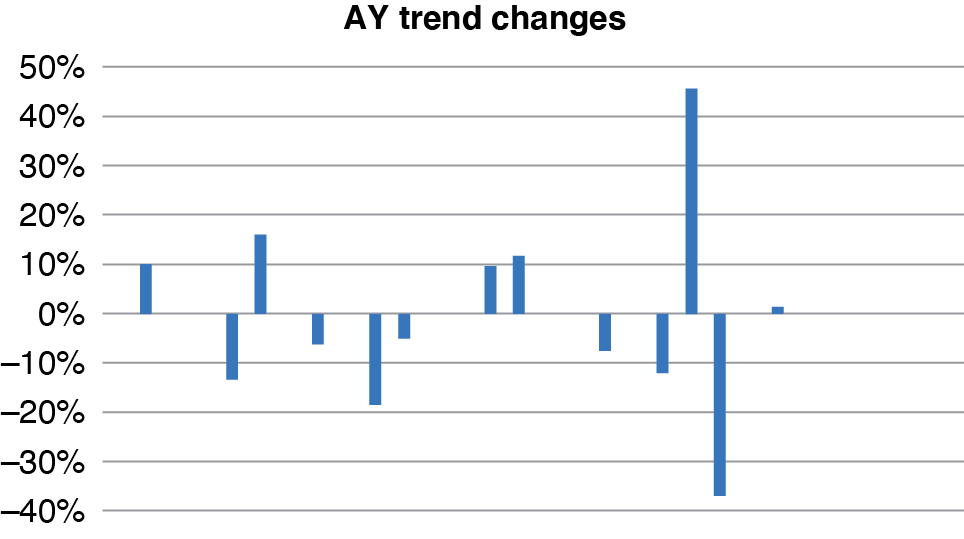
The fitted AY trend changes have more nonzero parameters, as seen in Figure 4.2.

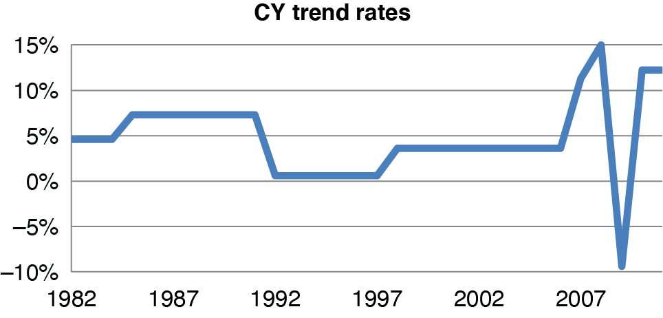
This model has 12 or 13 parameters to represent 32 accident years, which is reasonably parsimonious. Figure 4.3 shows the resulting fitted AY levels, unlogged. These are roughly at the level of first-year payments at 1980 cost levels. In recent years, losses are lower due to safety initiatives. Figure 4.4 is the CY fitted trends.

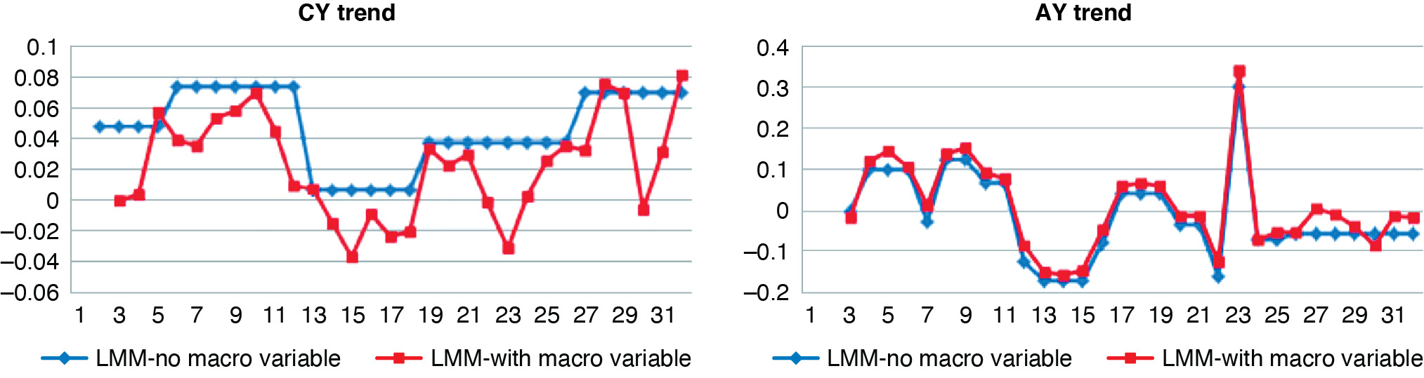
We also did a comparison of LMM estimates using fixed-point iteration versus MATLAB’s routine. For these we also excluded variables for trend changes in 2007–2009, effectively forcing those parameters to 0. That decision resulted in underestimating 2008 and overestimating 2009, but we felt it gave a better estimate of the recent trend levels for projection purposes. Figure 4.5 compares the fitted trends from both models as well as for the model that takes all the trend changes as fixed effects.

The fixed point–estimated AY trends are a bit lower, and CY trends a bit higher, than those obtained using the other models. With slight differences also in the DY trends, these model fits are very comparable at every point. The AY trends under MATLAB change a bit more and actually provide a bit better fit, but at the cost of using more nonzero parameters. The fact that AY and CY trends can largely offset, even though they do not fit every point exactly equally when they do so, is a common issue with PTF models. Experienced practitioners tend to ignore the individual trends and just look at their combination, but some reasonableness checks of CY trends in themselves would be useful, even if not strictly possible.

The all-fixed model shows a lot of fluctuation in CY trends, which neither LMM model recognizes. The LMM models, while a little different from each other, are very comparable and seem to be the result of different local maximums. SAS gives almost the same results as MATLAB. It would be nice to compare the joint likelihoods, with some adjustment for degrees of freedom, but there is a problem with doing so. The random-effect parameters that go to 0 also end up with very low variances, which increases their likelihood. These likelihoods can be very different with slightly different, very small variances, so they are often left out when computing the likelihood, but that creates a problem of arbitrary thresholds.

As an alternative, we look at the likelihood of the fitted y part of the model only, and compare by penalized likelihood for degrees of freedom. The diagonal of the hat matrix gives the number of degrees of freedom used, conditional on the variances. This is a starting point but is known to leave out the degrees of freedom used up in estimating the variances. We also tried a grind-out approach to estimating the degrees of freedom—change each observation slightly, one at a time, and refit the model, seeing how much the corresponding fitted value changes, which gives an estimate of the derivatives of the fitted values with respect to the actuals.

For the fixed-point estimation, the hat matrix shows it used 17.3 degrees of freedom, compared with 19.9 for MATLAB. These are nice small numbers, since the all-fixed model has 70 parameters, as does each of the fitted models if we count the parameters that are 0. However, using numerical derivatives, fixed-point estimation used 45.1 effective parameters (degrees of freedom), versus 50.7 for MATLAB. This is a surprisingly large increase. Since there are 275 observations, with the optimized variance parameters given, changing a data point, on average, changes the fitted point 7% as much (7% of 275 is 19.25). But when the variances are estimated as well, the fitted points move by about 18% of the change in the observations. There are 70 or so variance parameters, and it looks like, in this case, estimating them used up about 30 degrees of freedom. It always takes degrees of freedom to estimate variances, but usually in an informal way that often is ignored. In this case of mechanical model selection, the number of degrees of freedom used in the process is quantifiable.

How much penalty should these parameters get when comparing fits of this model using the various estimation methods? We use simplified versions of the AIC, BIC, and HQIC to investigate. Rather than multiply the negative log-likelihood (NLL) by 2, which gives an information distance, we just add a penalty to the NLL directly. For AIC, the penalty is 1 for each degree of freedom used, for BIC it is log(square root(sample size)), and for HQIC it is log(log(sample size)). The AIC has strong theory behind it but may tend to overparameterize in practice. The BIC sometimes seems to overpenalize, so we favor the HQIC basically for being somewhere in between, where the truth often lies. Close values, however, must be rated a tossup, as the penalty is mostly an approximation.

The sample size of 275 gives per-parameter penalties of 1.73 for HQIC and 2.81 for BIC. The NLL of the fit is –202.1 for the fixed-point model and –209.5 for MATLAB, which thus has the better fit. (In logs, the standard deviations were small, so the normal densities tended to be well over 1 over a small interval, actually making the log-likelihoods positive.) But after penalizing for the hat matrix parameter count, HQIC is –175 for MATLAB and –172 for fixed point, so MATLAB is only slightly better. When including the full parameter count, HQIC is at –124 for fixed point, which is now slightly better than the –122 for MATLAB. Thus these estimates really are quite similar in goodness of fit. Another test would be the small sample AIC, which for a sample of size n and k parameters, gives a penalty of nk/(n – k – 1). For 50 and 45 parameters, respectively, that would give penalties of 61.4 and 54, with a difference of 7.4, exactly canceling the NLL difference.

Companies and regulators have an interest in the impact of macro variables on losses, so we tried using such variables to model this triangle. What worked pretty well was to use the log of the personal consumption expenditures medical price index instead of the average CY trend as the fixed-effects CY variable, add the log of unemployment duration also as a CY variable, and add the detrended log of payroll as an AY variable. Detrending seemed to be necessary to avoid collinearity, and it also allowed us to keep the average AY level constant. Figure 4.6 shows the historical log of payroll and its trend, which is subtracted. In the fit of logged dependent variables on logged independent variables, parameters can be interpreted as elasticities, that is, the relative changes in observations due to a change in the variable. For medical costs, this parameter was 59%, which is fairly reasonable since that is close to the percentage of workers comp costs that are medical. The payroll effect was 1.08, which is interesting as some actuaries just assume it is 1.0 and divide losses by payroll as an exposure base. The unemployment duration had a parameter of –14%, which is not as large. Workers comp losses by AY are thought to go up with unemployment duration, but as a CY effect, the sign is ambiguous theoretically—injured workers might prefer to stay out longer or return to work sooner—so the empirical result is a finding in itself.

Figure 4.7 shows the AY and CY trends from this model and from the time-only model. Although the macro model allows estimation of how the losses would change in various economic scenarios and could rationalize reserve changes when there are economic changes, it does not have any better fit and would not necessarily give a better reserve estimate.

5. Mortality triangle example

Mortality research uses a bit different notation for the same models, so we will now shift to that notation. The primary modeling is by age at death, so we have lag, still denoted as d, and calendar year, which was w + d but here will be denoted as t. Then year of birth is t – d. The EPTF model can be written as

$$\log \left(M_{d, t}\right)=a_{d}+b_{d} h_{t}+c_{d} u_{t-d}+f_{t-d}+\varepsilon_{d, t} .$$

M is the ratio of deaths in the year to lives at the beginning of the year. For now we will model its log as normally distributed, but often the number of deaths is modeled as a Poisson or negative binomial^[2] distribution in M times the beginning lives. All of these parameters were fitted as trend changes after initial levels using LMM, as in the loss triangle case, here using a nonlinear optimizer in R to maximize the joint log-likelihood.

In this model, a is the mortality curve showing the increase in mortality rates at higher ages. The curve is close to linear on the log scale after about age 30. The trend toward lower mortality over time is expressed by h, but this trend is different at different ages and so is multiplied by an age effect, b. These two terms together form the original Lee-Carter mortality trend model, which actually picks up most of the variability in mortality over time.

Year-of-birth groups are called cohorts in this literature and tend to be quite strong factors in the UK, where a lot of this modeling has been done. And they have an impact in the United States as well. Some years of birth seem to have higher or lower mortality at all ages, perhaps depending on economic and climatic conditions when cohort members were young, or perhaps relating to ages reached at various societal milestones, such as the popularity of smoking or the arrival of medicines to reduce blood pressure. Anecdotally, for example, children born in Russia during the early years of World War II seem to have experienced higher mortality, perhaps due to the harsh conditions in their youth. The u parameters pick up a cohort effect that varies by age, and f is a constant cohort effect. The former is in the Renshaw-Haberman (2006) model, while the latter is the AY parameter in reserve models. We include them both and hope that parameter reduction will eliminate any overparameterization.

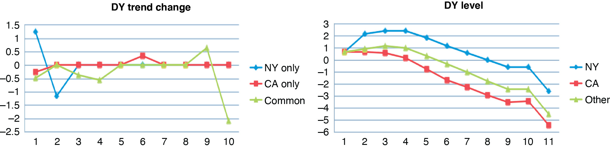
The Human Mortality Database has population mortality data for a number of countries. We were interested in modeling mortality trends for annuities, such as workers compensation permanent claims. The exposures for annuities are typically older ages, perhaps 55–99. However, as Venter (2011) and others note, estimating cohort effects is subject to a lot of parameter uncertainty unless enough observations are used for each cohort. Another restriction is that U.S. data is regarded as unreliable before 1970. For these reasons, we choose to model ages 16–99 for calendar years 1971–2010, which involved the birth-year cohorts 1881–1955. This gives 40 observations for both the 1955 cohort and age 99. The 84 ages were modeled with about 40 nonzero changes in trend for the mortality curve a_d, as shown in Figure 5.1.

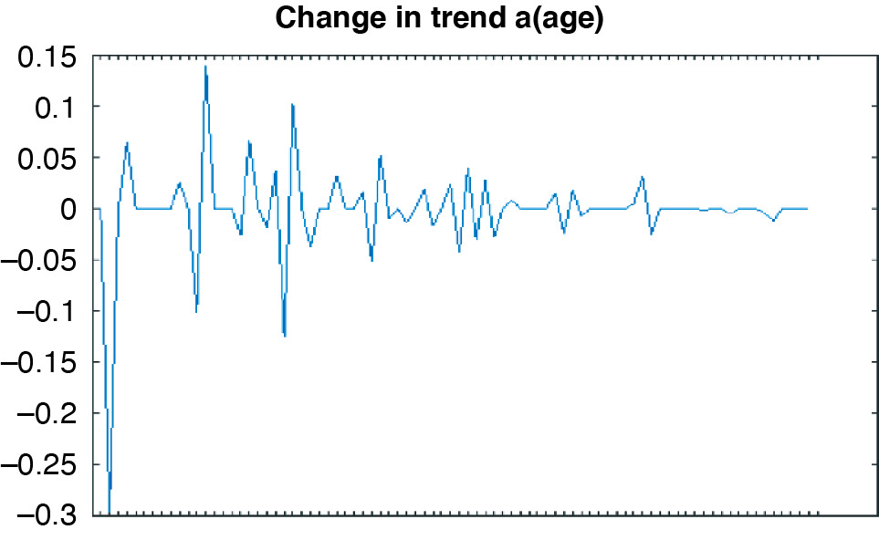
This estimation nonetheless produced a fairly steadily rising mortality trend after age 30, the slope shown in Figure 5.2. Figure 5.1 shows a few consecutive offsetting trend changes, for reasons not entirely clear. There appear to be a few milestone ages, such as 80, that people seem to be able to hang on to reach. In addition, changes between ages 16 and 30 may be related to risky behavior patterns. Some, though, might simply be random, and other parameter reduction methods, such as LASSO, may produce fewer of them.

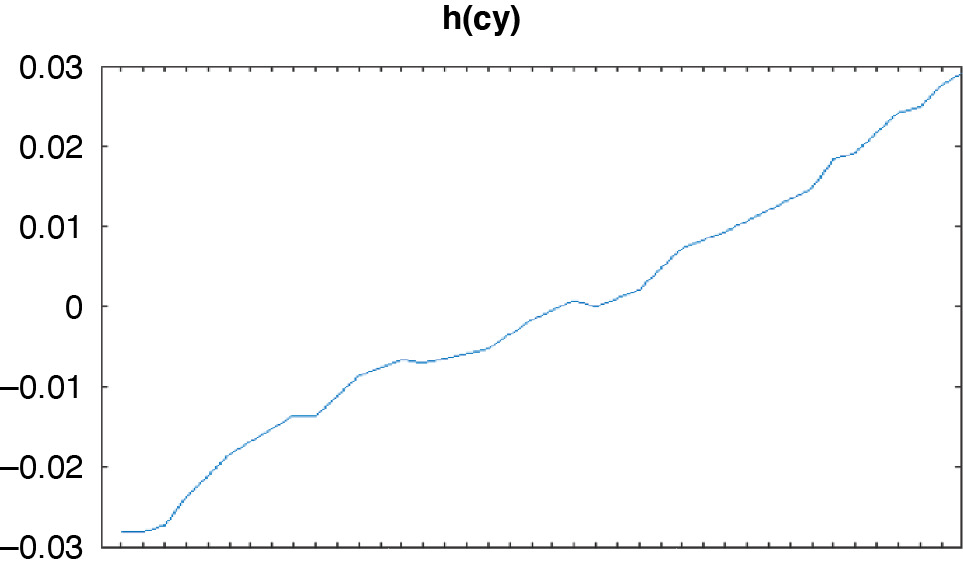
We modeled the mortality trend over the 40 years with about 25 trend changes (Figure 5.3).

The result was a fairly constant slope over time, but with many kinks (Figure 5.4).

The curve is upward sloping because it is multiplied by b, with the product generally coming out negative (Figure 5.5). This is an arbitrary outcome of the parameterization and could have been reversed. Again, there appears to be room here for further parameter reduction. The age multiplier, b, is actually stronger (here on a percentage basis) at the younger ages and appears to be largely gone by the late 90s.

The cohort parameters u (with age multiplier) and f, shown in Figures 5.6 and 5.7, respectively, tend to be a bit smoother and both center around 0, as does the cohort age multiplier c, shown in Figure 5.8. Apparently these have all had some parameter reduction applied.

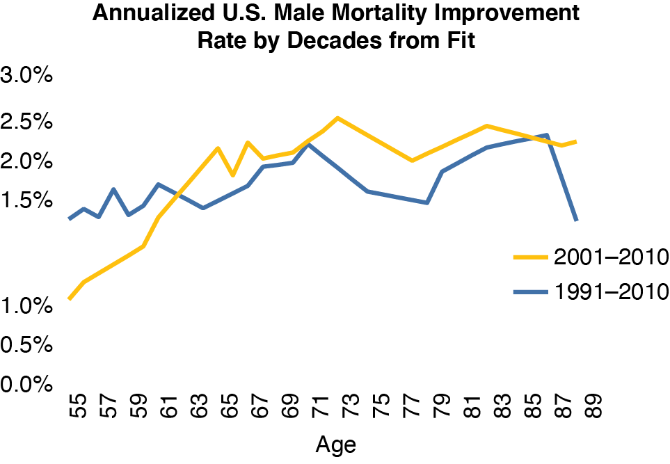
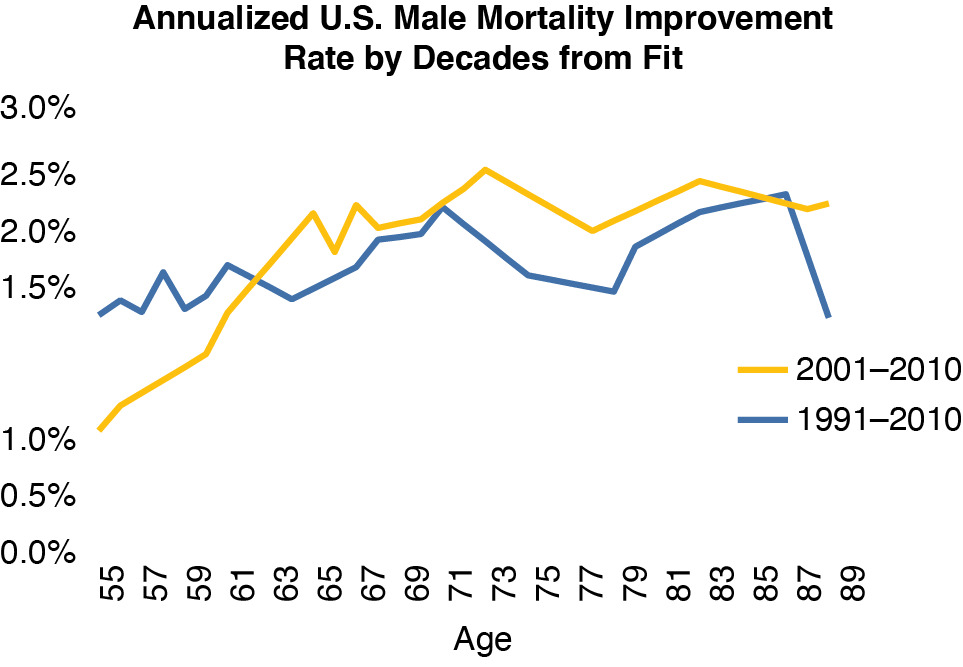
The bottom line is the combined effects of trend, age, and time, which we calculate as the trend rates for the fitted mortality rates from the model. Figure 5.9 shows the average mortality trend by age for the last 10 and 20 years, respectively. It looks to be 2%–2½% annually in the most critical age range. A 1916 workers comp permanent disability claim finally closed in 1991—it was being paid for 75 years. That accident was a hundred years ago, so with this kind of mortality trend, a comp claim that will receive benefits for a century is probably open already. Taking account of the mortality trend is one critical factor needed to get comp reserves right.

6. LASSO (least absolute shrinkage and selection operator)

LASSO provides another way to reduce the number of parameters in a model. Start with the linear model y = μ1_n + Xβ + ε. The mean times a vector of all 1s is modeled a little differently and therefore is shown separately. The LASSO estimate is the set of parameters that minimize NLL + λ∑|β_j| for a selected value of λ. This selection allows the modeler to control the degree of smoothing.

To make this a fair fight, all of the predictive variables are first standardized—that is, divided by their standard deviations after their means have been subtracted. That puts all the variables on the same scale. Each standard deviation just ends up in the coefficient, and all the mean impacts get into the estimate of μ, which is not included in the minimization of the sum of the parameters.

This is a little different than LMM in that there is only a single fixed effect, the mean. In the LMM triangle models, the AY-level starting variable has value 1 for all observations, so in regression terms, this is the overall mean. Experimenting with the other fixed-effects variables has shown that making them all random effects creates little change in their parameters, so setting up LMM with only the mean as a fixed effect works fine, and can thus translate to LASSO.

The choice of the smoothing factor may make LASSO seem less objective than LMM, but LMM involves choices as well. Just taking a normal distribution for each random-effect parameter is a choice in itself, as is assuming that these normal distributions are independent. Indeed it is not unusual for modelers to impose a correlation structure on the random effects to get more smoothing, which did in fact seem potentially useful in the tests above. In addition, there are approaches within LASSO to select the smoothing factor, typically cross-validation. A common way to do so is to fit n different models, each leaving out one of the n observations, and find the factor that does the best at this form of out-of-sample prediction.

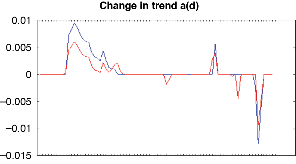
There are a number of statistical packages that do LASSO fitting, and we used MATLAB’s. It is pretty straightforward to do—the packages may even do the standardization for you. We illustrate the results here for the mortality fitting described in Section 5. A λ of around 10^–6 turns out to give parameters roughly comparable to LMM, so we look at additional smoothing by using 10^–4 and 10^–3 for comparison. In the charts, the red lines represent λ = 10^–4, and the blue lines are the smoother 10^–3, which tends to have fewer trend change parameters (i.e., more parameters at 0). Both of these are a fair bit smoother than LMM (Figure 6.1).

The resulting mortality curves are also a bit smoother than in LMM (Figure 6.2).

The time trend in mortality also loses a lot of its annual fluctuations in these models (Figure 6.3).

The fitted mortality time trend thus has less fluctuation in slope (Figure 6.4).

The trend multipliers by age end up with the same basic shape as but a lot smoother than LMM (Figure 6.5).

Cohort effects that vary by age were essentially eliminated in the LASSO tests (Figure 6.6). The cohort effects that are constant across ages for each year of birth were quite similar to those from LMM.

Sometimes mortality models use cubic splines across the parameters for smoothing, but the more statistically based approach described in this paper picks out the variables for which more or less smoothing would be appropriate, and it does not always end up with graphs that look like splines.

LASSO fitting to trend changes is easy with statistical packages and affords a choice of smoothing, so clearly it has a lot of potential for actuarial use. The different choices of λ give alternative models, for example, which are often needed in reserving. Using cross-validation to choose the degree of smoothing is also promising and is somewhat standard, but it is beyond the scope here.

7. Conclusions

Modeling trends in three directions is not needed if the cost trend is a constant over time, but otherwise it can provide a more accurate account of the development process than do other models. Some method for parameter reduction is usually applied when trends are modeled in this way. Reducing parameters also leads to better fits based on statistical fit measures that penalize for overparameterization even in row-column models. Nevertheless, parameter reduction has tended to be ad hoc.

LMM and LASSO provide methodologies for reducing the parameters in loss and mortality triangle models that are consistent with modern approaches in other areas of statistics. It is possible to do penalized likelihood calculations for these models using the method of generalized degrees of freedom, but this method is computationally extensive. Doing so for LMM revealed that the common approach of having a variance for each random effect uses a lot of degrees of freedom and thus is its own form of overfitting. Specifying only one variance parameter, or one for each direction, would possibly work better.

LASSO uses just one shrinkage parameter, which can be optimized by penalized likelihood with generalized degrees of freedom. A more common way of optimizing it is leave-one-out estimation, or LOO, in which the model is fitted sequentially on every subset of the data that omits a single observation, and then the sum of the NLLs of the omitted observations is optimized by choice of the shrinkage parameter. This method is also resource intensive, however.

The next logical step is to try Bayesian LASSO, which results in models similar to those of classical LASSO but provides a very fast method for numerical estimation of the LOO NLL. Thus it allows optimization of parameter shrinkage on out-of-sample observations.