Severity Curve Fitting for Long-Tailed Lines: An Application of Stochastic Processes and Bayesian Models

1. Introduction

Severity distributions are very important in actuarial science. They allow for the calculation of rating parameters such as increased limits factors and reinsurance costs. Fitting parametric curves to severity distributions is highly desirable for smoothing the data and adequately modeling tail losses. A difficult problem faced by actuaries is how to produce parametric or semi-parametric severity distributions representing ultimate settlement values for long-tailed lines of business where losses develop slowly over time.

For lines of business in which all claims and their ultimate values are known soon after occurrence, fitting a curve to the individual claim amounts is a straightforward exercise. For long-tailed lines, however, any finite set of individual claim data is biased due to the tendency for individual claim amounts to increase as the time since claim occurrence increases. Also, some claims are not reported until years after they occur, so the actuary’s dataset may not be complete and neither will they know if it is complete.

In this paper I will present evidence that a parameter fit to the severity distribution for each accident year and age will appear to follow a stochastic process. Then I detail a Bayesian hierarchical model which reasonably reproduces the theoretical true values for the critical parameters of the stochastic process when given a modestly sized simulated dataset. These critical values will give us estimates of trend, the ultimate severity distribution and excess layer losses. Finally, I will contrast with current methods.

2. Stochastic severity distribution parameters

2.1. Empirical evidence for the model

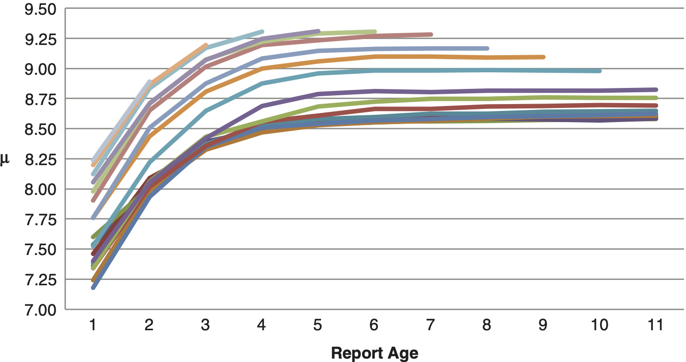
The method I will present in this paper was inspired by patterns found in actual data. Figure 1 shows the μ parameter of a lognormal distribution fit for each accident year and evaluation age from a grouped dataset of incurred amounts from commercial general liability claims. The number of claims in that dataset is on the order of hundreds of thousands. Lognormal was the best fit among about a dozen parametric distributions of one to four parameters. Each line is a single accident year.

Figure 1.Fitted lognormal by AY and age from large dataset of grouped liability claims.

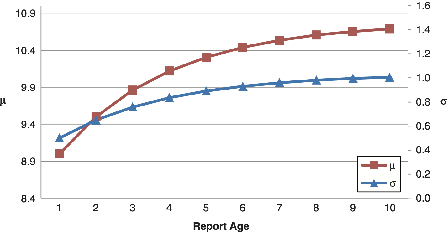
Figure 2 shows the μ parameters of a lognormal distribution fit to each accident year and age of a ground up dataset of approximately 3,000 individual professional liability claims.

The remainder of this paper will show how we can build a model around this pattern we see in the data. The purpose of the model is to solve the problem stated in the introduction: how to produce parametric or semi-parametric severity distributions representing ultimate settlement values for long-tailed lines of business where losses develop slowly over time.

Figure 2.Fitted lognormal by AY and age from dataset of professional liability claims.

2.2. Initial data and the basic model

The goal is to produce a parametric severity distribution representing sizes of loss for claims occurring in the prospective accident period. I’m assuming the user is starting with a dataset as shown in Table 1 with annual evaluations of individual claim amounts from a set of accident years.

As in the real-life examples of Section 2.1, suppose we observe individual claim incurred loss amounts for a given accident year for 10 years. At the end of each year we record the total incurred amount for every claim, whether open or closed, and then fit a parametric distribution, e.g., log-normal, to the claim amounts. This gives us 10 μ parameters and 10 σ parameters. Suppose we observe the pattern in Figure 3: each parameter appears to be following a smooth curve. By extrapolating the curves beyond the observation period, say to infinity, we will have an estimate for the distribution of ultimate settlement amounts.

Figure 3.Smooth curve of severity distribution parameter by report age.

These points can be fitted by exponential decay in the first differences, e.g., following the formulas:

$$\mu(t)-\mu(t-1)=\delta_{\mu} e^{-(t-1) / \theta_{1}}$$

$$\sigma(t)-\sigma(t-1)=\delta_{\sigma} e^{-(t-1) / \theta_{2}} .$$

Applying the geometric series formula to both sides, we have, for example:

$$\sum_{1}^{s} \mu(t)-\mu(t-1)=\mu(s)-\mu(0)$$

$$\sum_{1}^{s} \delta_{\mu} e^{-(t-1) / \theta_{1}}=\delta_{\mu} \frac{1-e^{-s / \theta_{1}}}{1-e^{-1 / \theta_{1}}}=\frac{\delta_{\mu}}{1-e^{-1 / \theta_{1}}}\left(1-e^{-s / \theta_{1}}\right) .$$

Defining

$$\Delta_{\mu}=\frac{\delta_{\mu}}{1-e^{-1 / \theta_{1}}}$$

as a closed-form solution to the above recursive relations, it can then be written as

$$\mu(t)=\mu(0)+\Delta_{\mu}\left(1-e^{-t / \theta_{1}}\right)$$

$$\sigma(t)=\sigma(0)+\Delta_{\sigma}\left(1-e^{-t / \theta_{2}}\right) .$$

Note that the Δ terms depend on θ and δ but not t. Now with these formulas we can determine the parameters of the ultimate severity distribution:

$$\lim _{t \rightarrow \infty} \mu(t)=\mu(0)+\Delta_{\mu}$$

$$\lim _{t \rightarrow \infty} \sigma(t)=\sigma(0)+\Delta_{\sigma}$$

This would give us an estimate of the ultimate average log-severity. We could also use these parameters to determine the amount of loss that would ultimately be in an excess layer or calculate ILFs.

2.3. Stochastic processes

A perfectly smooth curve is obviously an idealized model of the loss process and in reality will be subject to multiple layers of parameter risk. One risk is the potential for the actual severity distribution parameters to stray from the assumed deterministic path. The modern mathematical framework for random variables indexed by time like this is stochastic processes.

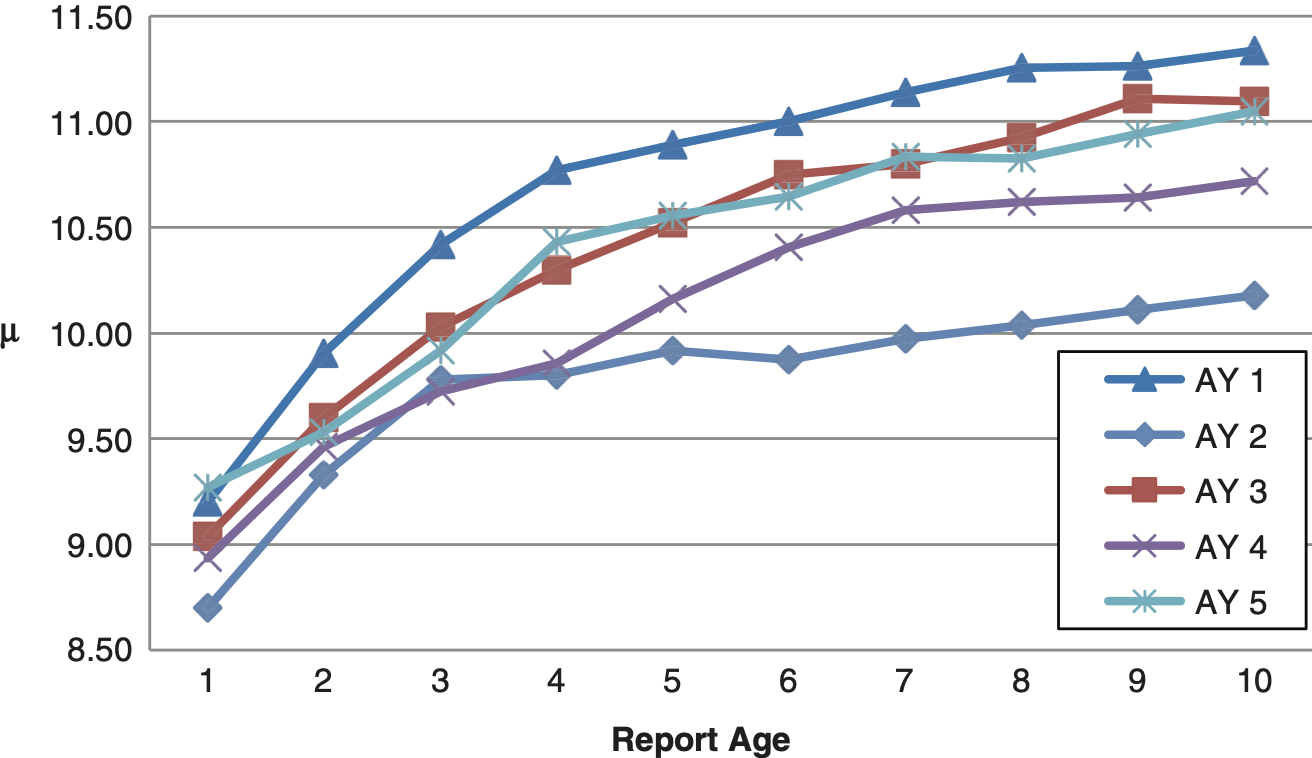
Suppose we observe multiple accident periods and see the pattern in the fitted log-normal mean parameters as shown in Figure 4, which more closely resembles the real data.

Figure 4.Smooth curve of severity distribution parameter with stochastic error.

The μ parameter still appears to follow a smooth curve but with a random error component between each reporting age. Also note that the paths appear to follow a moving average trend with drift, meaning each point is influenced by the prior points on the same graph, not the overall average among all paths. If we wanted to be more formal we could write the difference equation of the severity distribution parameters as

$$\mu(t)-\mu(t-1)=\delta_{\mu} e^{-(t-1) / \theta_{1}}+\epsilon_{\mu}(t)$$

$$\sigma(t)-\sigma(t-1)=\delta_{\sigma} e^{-(t-1) / \theta_{2}}+\epsilon_{\sigma}(t) .$$

With error variances that decay in time,

$$\operatorname{Var}\left(\epsilon_{\mu}(t)\right)=v_{\mu} e^{\left(-t / \eta_{1}\right)}$$

$$\operatorname{Var}\left(\epsilon_{\sigma}(t)\right)=v_{\sigma} e^{\left(-t / \eta_{2}\right)}$$

From here we could compute the ultimate severity distribution by taking limits of sums and also their variances by using stochastic calculus (beyond the scope of this paper).

2.4. Caveat on real-life sigma parameters

In the interest of full disclosure, the charts of the σ parameters for the real datasets in Figures 1 and 2 also follow what look like a stochastic process around a smooth curve, but the smooth curve is not as simple as the exponential decay model developed above. They look more like a bell curve with a local maximum within the first several years. For simplicity I will assume it does follow the exponential decay model, but if you look at real data, expect to see a more complicated pattern. The model developed in this paper can be expanded to handle other types of smooth curves. I would just urge the reader to visually inspect graphs of their data and fitted parameters to make sure your model is reasonable.

2.5. Trend, the link between accident years

So far we have seen multiple accident years together in Figures 1, 2, and 4, but we have only given formulas for a single accident year. A complete model must incorporate the data from multiple accident years simultaneously. This can be done by assuming all accident years follow different realizations of the same stochastic process, as in Figure 4. Additionally, we can incorporate the traditional assumption that losses in each successive accident year will be higher than the previous by a fixed rate of inflation, or trend.

Using the notation μ(i, j) where the first variable is the accident year and the second is the report age, we can incorporate trend very simply as follows:

$$\mu(i, 1)=\mu(i-1,1)+\text { trend } .$$

Equivalently, if we define μ to be a fixed number representing a baseline value for μ at accident year 0 and age 1, then we can write

$$\propto(i, 1)=\propto+\text { trend } * i .$$

In our final model below, we will also add a random error term to each μ(i, 1).

3. Application of Bayesian statistics

3.1. Extension to the small or medium dataset case

Even with a large volume of data, there will always be a range of possible estimates for the parameters of the smooth curve, the error variances, and all the other parameters of the stochastic process. This is the parameter risk of the stochastic model. How can we confidently use this model when we don’t have a very large dataset?

Instead of taking our small- to medium-sized dataset and trying to fit a model from scratch, we can start with an a priori set of possible models and use the data to modify the probability that each model is correct. The modern tool for this type of statistical analysis is a Bayesian hierarchical model. An excellent reference is Zhang, Dukic, and Guszcza (2012).

To put our stochastic process in the framework of a Bayesian hierarchical model, instead of simply saying the accident year inflation rate of the μ parameter is 5% per year, we specify that it is normally distributed with mean 5% and standard deviation 1%, or that the exponential decay of the first differences in the σ parameter isn’t 30%, but normally distributed with mean 30% and standard deviation 5%. These are our prior distributions. Then, given a dataset of individual claim amounts indexed by accident year and report age, we can calculate the Bayesian posterior distributions of all our severity distribution stochastic process parameters.

3.2. Bayesian hierarchical model of stochastic severity development

I created an implementation of this model in Stan, a free and open-source R package for building Bayesian models and calculating posterior estimates. The full code of the model can be found in Appendix A. For readers who are not familiar with Bayesian modeling and would like more background, an excellent reference is Scollnik (2001).

I assume that claims in each accident year and age are log-normally distributed with the μ and σ parameters following discrete time stochastic processes defined by the following formulas.

$$\mu(i, 1)=\mu_{\text {start }}+\text { trend } * i+\epsilon_{\mu}(i, 1)$$

$$\sigma(i, 1)=\sigma_{\text {start }}+\epsilon_{\sigma}(i, 1)$$

$$\mu(i, j)=\mu(i, j-1)+\mu_{\text {incr }} * e^{-(j-1) / \mu_{\text {growh }}}+\epsilon_{u}(\mathrm{i}, \mathrm{j})$$

$$\sigma(i, j)=\sigma(i, j-1)+\sigma_{\text {incr }} * e^{-(j-1) / \sigma_{g r o w h}}+\epsilon_{\sigma}(\mathrm{i}, \mathrm{j})$$

$$\boldsymbol{\epsilon}_{\mu}(i, j) \sim N\left(0, p_{\mu} * e^{-(j-1) * *_{\mu}}\right)$$

$$\boldsymbol{\epsilon}_{\mathrm{\sigma}}(i, j) \sim N\left(0, p_{\sigma} * e^{-(j-1) * r_{\sigma}}\right) .$$

Explanations of each variable are given in Table 2.

The input data, shown in Appendix B, represents 20 claim amount observations per accident year and report year from the upper half of a 10 by 10 accident year/report year triangle. There will be 10 report ages observed from the oldest accident year and only one from the most recent. The result is 1,100 data points. The data is simulated randomly from a process identical to the model so that we know the answer and can compare the Bayesian posterior estimates with the true theoretical values.

I have assumed mostly uninformative uniform distributions over wide ranges relative to the true parameter values for purposes of this example. In a real application, the true benefit of this model is the ability to use an informative prior. For example, if 10 similar datasets have been analyzed and μ_growth appears to be normally distributed with mean 5 and standard deviation 2, then that would be a reasonable prior to use in analyzing the 11th dataset. Even for a brand new dataset, there is likely some type of expectation by the analyst of the range of parameters and the prior is how those expectations enter the model.

In this example, the priors for μ_start and σ_start are very specific, however. These variables represent the parameters of the distribution of claims at the first reporting age. Since these claim amounts are immediately available, this is a classical fitting exercise. I assume the variance between our estimate and the true values (9 for μ_start and 0.5 for σ_start) is given by Fisher’s information; see Example 15.9 in Klugman, Panjer, and Willmot (2008).

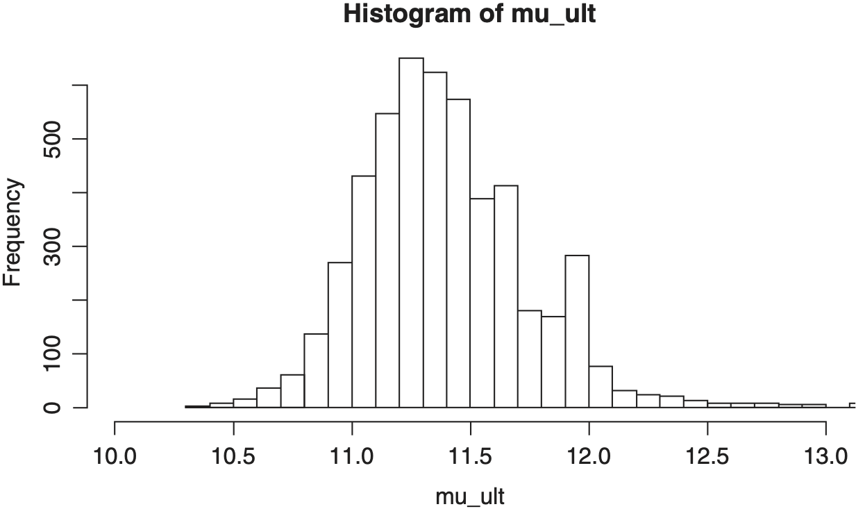
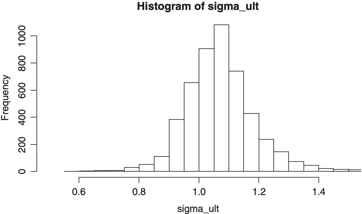
Near the end of the code I define the outputs of interest, μ_ult and σ_ult. These are calculated by extrapolating the smooth curve out to report time infinity. We are not limited to the estimate for μ(i, 10) or σ(i, 10).

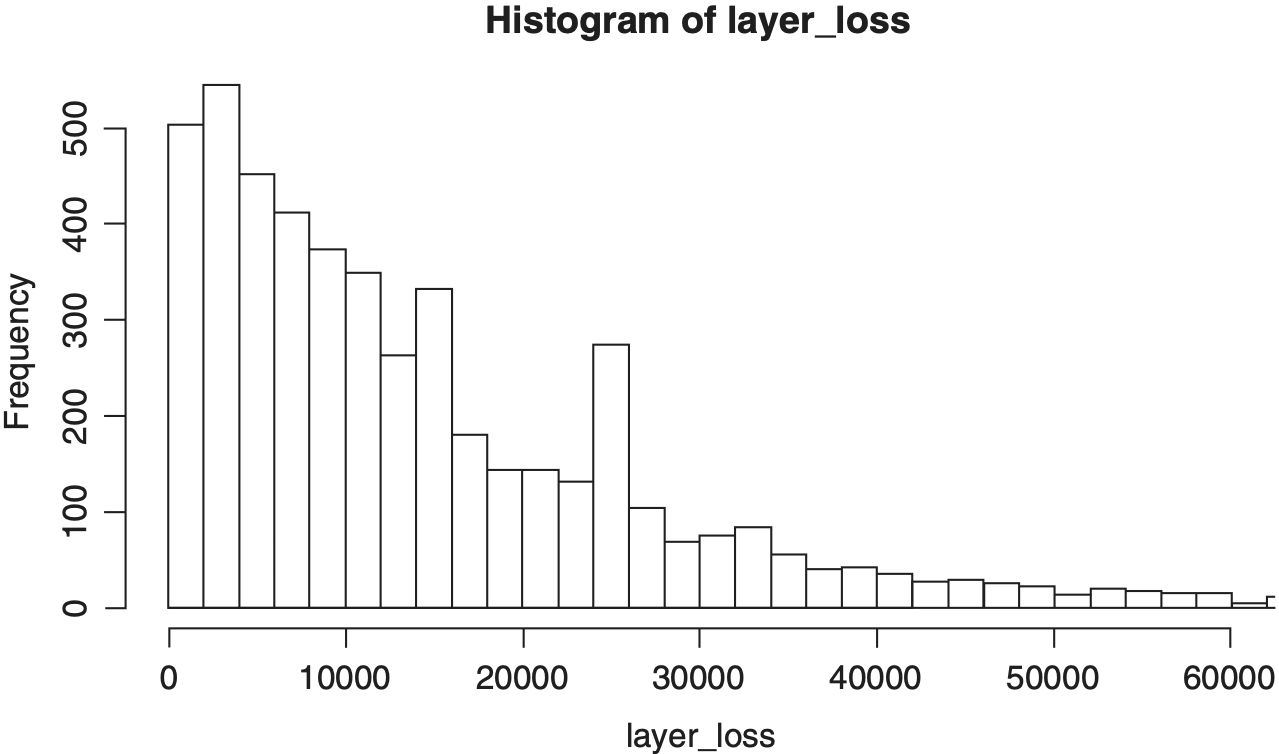
Finally, we calculate the expected layer loss and frequency to a $1M excess $1M layer for the next accident year. The output is an approximation to the Bayesian posterior distribution of the expected layer loss. Note that this is per claim since the model does not have a frequency component.

3.3. Model output and performance

Table 3 summarizes the model output and compares the posterior estimates to the true values used to simulate the data.

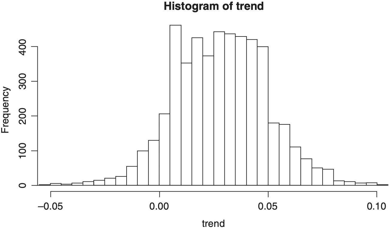
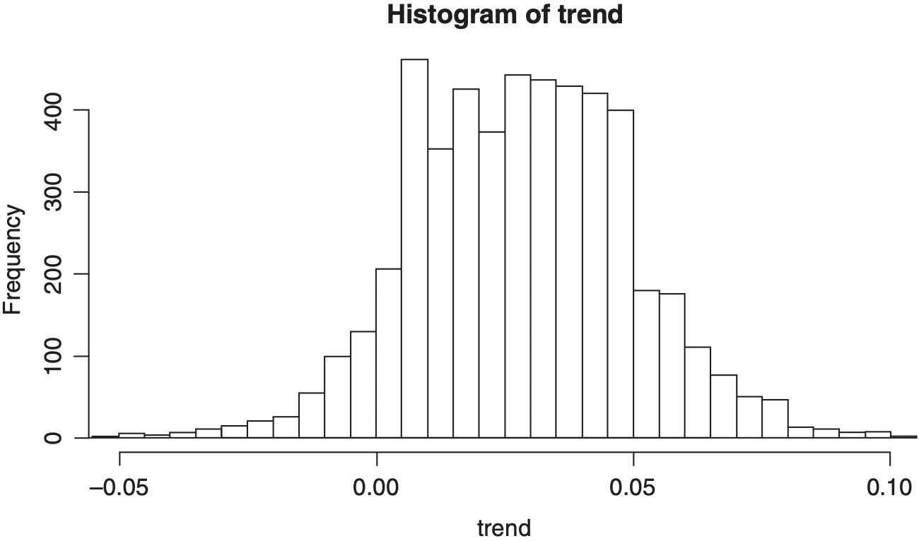
Table 3 shows the model coming within approximately one standard deviation of the true value for the critical output parameters of μ_ult, σ_ult and trend, but the posterior means differ somewhat from the true values. The point is not that the model can exactly reproduce the true parameter values but that in the case of a small- to medium-sized dataset the model is able to produce a reasonable estimate of the stochastic process parameters and also give an estimate of the uncertainty around those estimates. The posterior means will be closer if we either have more data or supply informative priors.

Since μ_ult and σ_ult are stochastic, they do not have a true value but rather a true mean. For any combination of these variables, we will get a different layer loss and frequency which is why the “true value” is ambiguous. Parameter variance in the model for ground up losses becomes leveraged and adds to the expected layer loss and frequency; therefore, the expected value depends on which types of parameter risk are considered to be contributors. As defined in the code, layer_loss and layer_freq depend only on μ_ult, σ_ult and the trend and the model means reflect the uncertainty in those parameters. One could argue that they should also depend on the process variance of a generic accident year, introducing p_μ and p_σ into the equation.

Figures 5 through 8 show histograms of the posterior distribution of the critical output variables.

Figure 5.Histogram of posterior mu_ult.

Figure 6.Histogram of posterior sigma_ult.

Figure 7.Histogram of posterior trend.

Figure 8.Histogram of posterior layer_loss.

4. Survey of current methods

4.1. ISO: Fitting by closure age

ISO provides ultimate severity distributions for many long-tailed liability lines of business. Their method of accounting for severity development is to fit a distribution to claims closed at each reporting age, then weight those curves together by the proportion of claims expected to be settled in each age. Once a claim is closed, then the loss amount is fixed, so there is no bias in the fit to the data for a given closure period.

In the later ages the data thins out and there may be a problem fitting credible curves. ISO’s solution is to group all closed claims beyond a certain age together and give them a single severity distribution. Industry excess loss triangles would indicate that this assumption is not accurate, but it may be immaterial for the volume of data and number of years ISO has available. For an application with less data or a shorter history, it may be necessary to make explicit adjustment for development beyond the reporting ages observed.

4.2. NCCI: Claims dispersion

The method put into practice by the NCCI and WCIRB for fitting ultimate severity distributions for worker’s compensation losses is claims dispersion; see Corro and Engl (n.d.) and California WCIRB (2012). The basic idea behind claims dispersion is, given a claim amount, we can find the distribution of the ultimate settlement value by looking at the historical movement of individual claims over time. The aggregation of the ultimate settlement distribution for each current claim gives the ultimate severity distribution.

If we are working with a low to medium volume of data, it may not be possible to fit two or more parameters between every reporting age independently. Also, if the average IBNR claim is larger than the average previously reported claim, then some of the severity distribution development cannot be captured by measuring the change in existing claims.

4.3. Bayesian methods

An excellent application of Bayesian statistics to the fitting of loss distributions is given in Meyers (2005). Given a multitude of possible full severity distributions, Meyers uses the observed claim experience along with Bayes’ Theorem to calculate posterior probabilities that each model is correct, then uses these probabilities to calculate the expected layer loss.

Meyers acknowledges the loss development problem and proposes a solution in which each possible loss model has an early report distribution and a corresponding ultimate loss distribution. The Bayesian calculation is done using the immature individual loss data and the early report severity curves, then the same posterior probabilities are given to the corresponding ultimate severity distributions. Construction of the ultimate severity distributions associated to immature report distributions is not described.

4.4. Stochastic models

The papers by Drieksens et al. (2012) and Korn (2015) develop more detailed stochastic models of the claims process in order to calculate reserve distributions and more. They use multiple evaluations for each claim, paid and incurred amounts, open/closed status and separate treatment of IBNR claims in a detailed stochastic framework that mimics the actual movement of individual claims.

Drieksens recognizes the need for a tail factor to account for development beyond observed ages, but the determination of the factor is left to ad hoc methods. Korn discusses two methods for determining severity distributions based on a Cox proportional hazard model in a generalized linear model framework with semi-parametric distributions. These appear to be very robust approaches, although they may suffer in cases of low data volume unless enhanced with Bayesian credibility, as suggested by the author.

5. Conclusion

We saw evidence from actual data that when we observe a fitted parameter to the severity distribution for each single accident year and age, it will appear to follow a smooth curve with some random error. I formulated this more precisely in terms of stochastic processes. Then I showed how a Bayesian hierarchical model can reasonably reproduce the theoretical true values for the critical parameters of the stochastic process when given a modestly sized dataset of individual claim amounts at multiple evaluations. Readers now have at their disposal a new method for developing ultimate severity distributions for long-tailed lines of business.

Beyond simply being an additional method, I believe the “Bayesian stochastic severity” framework has many benefits over currently available methods. Our method has very minimal data requirements. Data in the format of Table 1 is required, although we never actually use the information on the movement of an individual claim. Only triplets of (accident year, report age, incurred amount) are necessary.

Although the link between reports for each individual claim is lost, data from multiple accident years and report ages are used simultaneously in a unified and visually intuitive way through the stochastic process. The smooth curve portion is easy to communicate and compare between applications.

The Bayesian model responds appropriately to the volume of data provided, hence we can proceed with a small- to medium-sized dataset. If the dataset is limited in time, the method explicitly accounts for development beyond the latest observed report age. With a limited number of accident years, minimal information on trend is available and the model will fail to update the posterior significantly from the prior, which is a good thing in that case.

Finally, I am providing readers with full computer code and sample dataset for easy reproduction of the results presented and the ability to conduct further experimentation.