Validating the Double Chain Ladder Stochastic Claims Reserving Model

1. Introduction

A crucial function in the management of an insurance company is that of estimating the future outstanding liability of past claims, which may have been incurred but not yet reported (IBNR) or reported but not settled (RBNS). The function holder is most likely to be an actuary who will use not only his technical expertise but also a significant amount of professional judgement to accurately quantify the value of the liability that should be recorded as technical reserves in the company financial statements.

Insurance claims characteristics vary by their nature, timing, amount, reporting delay, and settlement delay. For example, property damage claims are more likely to be short-tailed, i.e., paid quickly. Industrial claims however, are long-tailed, i.e., they take much longer to be fully settled. This means that the methodology that should be used for quantifying those claims cannot reasonably be expected to be exactly the same. The actuary will choose the most adequate method for each situation. One of these methods is the classical chain ladder method (CLM). CLM was conceived as a deterministic method that operates on the historical data contained in the so-called run-off triangles. The simplicity and the intuitive appeal of CLM have made it one of the most applied methods in practice by actuaries. But actuaries are aware of many of the limitations and drawbacks of CLM, such as its reliance on a small dataset and its possible instability.

Over the past decades, a number of research articles have appeared which aim to replicate the CLM forecasts in a statistical framework with the added benefit of calculating the variability around the mean estimates. Mack (1991), Verrall (1991) and recently Kuang, Nielsen, and Nielsen (2009) have identified the CLM forecasts as classical maximum likelihood estimates under a Poisson model. See England and Verrall (2002) and Wüthrich and Merz (2008) for comprehensive reviews of stochastic claims reserving.

In this paper we will focus on the double chain ladder (DCL) model proposed by Martínez-Miranda, Nielsen, and Verrall (2012). The DCL model is a statistical model that can replicate the classical chain ladder estimates by using a particular estimation method. But it can also be used to provide further results that classical chain ladder is unable to provide, such as the prediction of outstanding liabilities separately for RBNS and IBNR claims, and the prediction of the tail which is defined as the claims forecasts with development process beyond the latest development years observed.

The DCL method which replicates the CLM forecasts uses only two observed run-off triangles. One triangle consists of the number of reported claims, and the other is the so-called paid triangle: the total paid amounts by underwriting and development year. The DCL method can therefore be viewed as a link between classical reserving and the statistical model, in that it uses the non-statistical calculation method but it also has a full statistical method. However, it is well known that the classical CLM estimates tend to be unstable in the more recent underwriting years. This instability leads in many cases to an unacceptable forecast for the total reserve. The Bornhuetter-Ferguson technique is one of the most common ways to correct that problem in practice. Martínez-Miranda, Nielsen, and Verrall (2013) point out that the instability comes from the estimation of the underwriting inflation parameter in the DCL model. Note that that paper (and any method based on paid data) ignores the case estimate reserves from the claims adjusters (the “expert knowledge”). Taking the spirit of the Bornhuetter-Ferguson technique, the authors describe another method to estimate the DCL model which corrects the instability of the DCL forecasts. The method is called Bornhuetter-Ferguson double chain ladder (BDCL) and it works on the same triangles as DCL together with an additional so-called incurred claims data triangle. The case estimates contained in the incurred data are considered as prior knowledge that can indeed provide more stable estimates of the underwriting inflation. Although the BDCL works on the incurred claims data triangle, the BDCL reserve estimate is different from the incurred chain ladder reserve which is calculated by applying CLM to the incurred data triangle. Being aware of the popularity of the incurred chain ladder reserve among many actuaries, in this paper we introduce a third method to estimate the double chain ladder model that can exactly replicate that reserve estimate. We will call this method incurred double chain ladder (IDCL). Berquist and Sherman (1977) also consider triangle adjustments.

The purpose of this paper is therefore to explore a link between mathematical statistics and reserving practice in insurance companies. This will add value to practitioners who might be interested in evaluating the robustness of the reserving risk used to compute the best estimate liability for Pillar 1 of the Solvency II framework. Alternatively, the method could be used to assess the strength of case estimates philosophy because the output is split between IBNR and RBNS reserves or outstanding claims reserve.

The paper is structured as follows. In the next section we describe the double chain ladder model. In Section 3 we define three methods to estimate the model parameters, referred to above as DCL, BDCL and IDCL. In Section 4 we describe how to calculate the outstanding liabilities forecasts once the double chain ladder model parameters have been estimated. We illustrate the methods using two real datasets: a motor personal injury (Motor BI) portfolio and a motor fleet property damage (Motor PD) portfolio. In Section 5, we discuss the advantages and disadvantages of the three methods and support the decision in practice among them using formal model validation. In this section we also explore and validate any additional improvement gained by a common practice by actuaries consisting of limiting the data used to estimate the model to just the more recent calendar years. Some final remarks in Section 6 conclude the paper.

2. The data and model

In this section we will briefly describe the double chain ladder model, introduce the notation and state the assumptions needed for consistent estimates. For a more detailed description we refer to Martínez-Miranda, Nielsen, and Verrall (2012, 2013). For a better understanding, afterwards, we will give a heuristic interpretation of these technically introduced parameters. We start with the introduction of some notation.

Let us assume that the number of years of historical data available is m. We also assume that our data is available in a triangular form I = {(i, j) | i = 1, . . . , m; j = 0, . . . , m − 1; i + j ≤ m}. Here, i denotes the accident or underwriting year and j denotes the development year. We will consider three triangular sets of data:

1. Numbers of incurred claims:N_m = {N_ij | (i, j) ∈ I}, where N_ij is the total number of claims of insurance incurred in year i which have been reported in year i + j.

2. Aggregated payments:X_m = {X_ij | (i, j) ∈ I}, where X_ij is the total payments from claims incurred in year i which are settled in year i + j.

3. Aggregated incurred claim amounts: \(\Theta_m=\left\{\Theta_{i j} \mid(i, j) \in I\right\}\), where \(\Theta_{i j}\) is the total incurred amounts originating from year i which have been reported before year i + j.

Note that in contrast to N_m and X_m, Θ_m is not real data but rather a mixture of data and expert knowledge since it is not fully observed yet.

Double chain ladder is based on micro-level data assumptions. We therefore define some variables which may not be observed. We denote the count of future payments originating from the N_ij reported claims, paid with k years settlement delay by N_ijk^PAID, ((i, j) ∈ I, k = 0, . . . , m − 1). Let \(Y_{i j k}^{(h)}\left(h=1, \ldots, N_{i j k}^{P A I D}\right)\) be the individual settled payments from the number of future payments N_ijk^PAID. Finally, denote by X^j_il those payments of X_il which are reported with delay less than or equal to j. We derive the decomposition

\[ X_{i j}=\sum_{l=0}^j \sum_{h=1}^{N_{i, l, i l l}^{p, l i}} Y_{i, j, l, l}^{(h)} . \]

Note that in order to obtain point estimates, it is not necessary to consider distributional assumptions, since moment assumptions are sufficient. The assumptions of the DCL model are as follows.

Assumptions A (cf. Martínez-Miranda, Nielsen, and Verrall (2012, 2013)).

1. Conditional on the number of incurred claims (N_ij), the expected number of payments with payment delay k is given by

   \[ \boldsymbol{E}\left[N_{i j k}^{P A D} \mid N_{m}\right]=N_{i j} \boldsymbol{\pi}_{k} \]

2. Conditional on the future number of payments (N_ijk^PAID), the expectation of the individual payments are given by

   \[ \boldsymbol{E}\left[Y_{i j k}^{(h)} \mid N_{i j k}^{P A I D}\right]=\mu \gamma_{i} \]

3. The incurred claim amounts can be described via

   \[ \Theta_{i j}=\sum_{l=0}^{m-1} \boldsymbol{E}\left[X_{i l}^j \mid \mathcal{F}_j^{(i)}\right] \]

   where \(\mathcal{F}_j^{(i)}\) represents the knowledge of the people making the case estimates at time i + j.

For the purpose of estimating the parameters we will need further assumptions. These assumptions go back to Mack (1991), who identified the multiplicative structure assumption underlying the CLM.

Assumptions CLM (cf. Mack (1991))

1. The number of incurred claims N_ij is a random variable with mean

   \[ \boldsymbol{E}\left[N_{i j}\right]=\boldsymbol{\alpha}_{i} \boldsymbol{\beta}_{j}, \quad \sum_{j=0}^{m-1} \beta_{j}=1 . \]

2. The aggregated payments X_ij is a random variable with mean

   \[ \boldsymbol{E}\left[X_{i j}\right]=\tilde{\boldsymbol{\alpha}}_{i} \tilde{\beta}_{j}, \quad \sum_{j=0}^{m-1} \tilde{\beta}_{j}=1 . \]

3. The aggregated incurred claim amounts \(\Theta_{i j}\) is a random variable with mean

   \[ \boldsymbol{E}\left[\Theta_{i j}\right]=\tilde{\boldsymbol{\alpha}}_{i} \breve{\boldsymbol{\beta}}_{j}, \quad \sum_{j=0}^{m-1} \breve{\boldsymbol{\beta}}_{j}=1 . \]

The parameters can be interpreted heuristically as follows.

• \(\alpha_i\) = the ultimate number of incurred claims for accident year i,

• \(\beta_j\) = the proportion of the ultimate number of incurred reported in the j’th development year,

• \(\tilde{\alpha}_i\) = ultimate aggregate claims paid in accident year i,

• \(\tilde{\beta}_j\) = the proportion of aggregated payments in the j’th development year,

• \(\check{\beta}_j\) = the proportion of aggregated claims incurred in the j’th development year,

• \(\pi_k\) = the proportion of claims settled after k years,

• \(\mu\) = the average cost of claims paid in the first accident year.

• \(\gamma_i\) = the claim severity inflation parameter, i.e., the average inflation of aggregated payments for accident year i.

The parameters in the CLM assumptions (i.e., \(\alpha_i, \beta_j, \tilde{\alpha}_i, \widetilde{\beta}_j, \check{\beta}_j\)) can be estimated using the traditional CLM method, which gives the maximum likelihood estimates. To estimate the parameters in assumptions A (i.e.,\(\mu, \gamma_i, \pi_k\)), we will use the following equations.

\[ \boldsymbol{E}\left[X_{i j}\right]=\alpha_{i} \gamma_{i} \mu \sum_{k=0}^{j} \beta_{j-k} \pi_{k} . \tag{2.1} \]

\[ \boldsymbol{E}\left[\Theta_{i j}\right]=\alpha_{i} \gamma_{i} \mu \bar{\beta}_{j}, \tag{2.2} \]

where \(\bar{\beta}_j=\sum_{h=0}^j \beta_h\) only depends on j.

In the next section we will describe in detail three different methods to derive these estimates.

3. Estimating the parameters in the double chain ladder model

To estimate the outstanding liabilities for RBNS and IBNR claims, the parameters in the model described in Section 2 should be estimated from the available data. In this section we describe three different estimation methods to achieve this goal: DCL, BDCL and IDCL. The three methods operate on classical run-off triangles and make use of the simple chain ladder algorithm.

3.1. The DCL method

The DCL only uses real data. That is only the two triangles N_m and X_m. Thus, it does not take use of knowledge of the experts, that is, \(\Theta_m\). Note that this also implies that assumptions A3 and CLM3 are not needed.

As implied by the name double chain ladder, the classical chain ladder technique is applied twice. We use the simple chain ladder algorithm applied to the triangle of the number of incurred claims N_m and the triangle of aggregated payments X_m to derive the development factors. These development factors lead to the two sets of estimators of \(\left(\alpha_i, \beta_j\right)\) and \(\left(\tilde{\alpha}_i, \tilde{\beta}_j\right)\) (i = 1, . . . , m; j = 0, . . . , m − 1).

For illustration, given the triangle N_ij the estimates are derived as follows (cf. Verrall (1991)):

\[ D_{i j}=\sum_{k=1}^{j} N_{i k}, \quad \text { (cumulative entries) } \]

\[ \hat{\lambda}_{j}=\frac{\sum_{i=1}^{n-j+1} D_{i j}}{\sum_{i=1}^{n-i+1} D_{i, j-1}}, \quad \text { (development factors) } \]

\[ \hat{\boldsymbol{\beta}}_{o}=\frac{1}{\prod_{l=1}^{m-1} \hat{\lambda}_{l}}, \quad \hat{\boldsymbol{\beta}}_{j}=\frac{\hat{\lambda}_{j}-1}{\prod_{l=1}^{m-1} \hat{\lambda}_{l}}, \quad \text { for } j=1, \ldots, m-1 . \]

The estimates of the parameters for the accident years i can be obtained by “grossing-up” the latest cumulative entry in each row. Thus, the estimate of \(\alpha_i\) can be obtained by

\[ \hat{\alpha}_{i}=\sum_{j=0}^{m-i} N_{i j} \prod_{j=m-i+1}^{m-1} \hat{\lambda} j . \]

Similar expressions can be used for the parameters of the aggregated paid claims triangle.

Alternatively, analytical expressions for the estimators can also be derived directly (rather than using the chain ladder algorithm) and further details can be found in Kuang, Nielsen, and Nielsen (2009).

Once the chain ladder parameter estimates are derived, applying assumption CLM2 to (2.1) yields

\[ \begin{array}{c} \alpha_{i} \mu \gamma_{i}=\tilde{\alpha}_{i}, \\ \sum_{k=0}^{j} \beta_{j-k} \pi_{k}=\tilde{\beta}_{j} . \end{array} \]

Then we solve the following linear system to obtain the parameters \(\hat{\pi}=\left\{\hat{\pi}_k \mid k=0, \ldots, m-1\right\}\).

\[ \left(\begin{array}{c} \tilde{\tilde{\beta}}_{0} \\ \vdots \\ \hat{\tilde{\boldsymbol{\beta}}}_{m-1} \end{array}\right)=\left(\begin{array}{ccc} \hat{\boldsymbol{\beta}}_{0} & \cdots & 0 \\ \vdots & \ddots & \vdots \\ \hat{\boldsymbol{\beta}}_{m-1} & \cdots & \hat{\boldsymbol{\beta}}_{0} \end{array}\right)\left(\begin{array}{c} \pi_{0} \\ \vdots \\ \pi_{m-1} \end{array}\right) \]

We also have

\[ \gamma_{i}=\frac{\tilde{\alpha}_{i}}{\alpha_{i} \mu} . \]

Since the model is over-parameterized, we define the identification γ₁ = 1 and the estimate μ̂ can be obtained from

\[ \hat{\mu}=\frac{\hat{\tilde{\alpha}}_{1}}{\hat{\alpha}_{1}} \]

Finally we can deduce the estimator \(\hat{\gamma}_i^{D C L}\) from the equation

\[ \hat{\gamma}_{i}^{D C L}=\frac{\hat{\tilde{\alpha}}_{i}}{\hat{\alpha}_{i}} \]

We have now derived all final parameter estimates \(\hat{\alpha}_i, \hat{\beta}_j \hat{\mu}, \hat{\gamma}_i^{D C L}, \hat{\pi}_k \mid k=0, \ldots, m-1, i=1, \ldots, m, j=0, \ldots, m-1\}\). However, note that having some distributional assumptions in mind, one might like to have positive delay parameter estimates, \(\hat{\pi}_k \geq 0\), and also that they sum up to\(1, \sum_{k=0}^{m-1} \hat{\pi}_k=1\), which is generally not the case. Thus, we will also define adjusted delay parameter estimators (\(\hat{\tilde{\pi}}_k\)). We believe that the following simple method will provide reasonable estimates in most cases, but we note that more complicated approaches like constrained estimation procedures are also possible. We introduce a maximum delay period d as the smallest integer with the property to satisfy \(\sum_{k=0}^{d-1} \max \left(0, \hat{\pi}_k\right) \leq 1 \leq \sum_{k=0}^d \max \left(0, \hat{\pi}_k\right)\). Then, we define

\[ \hat{\tilde{\pi}}_{k}=\left\{\begin{array}{ll} \max \left(0, \hat{\pi}_{k}\right) & \text { if } k=0, \ldots, d-1, \\ 1-\sum_{k=0}^{d-1} \max \left(0, \hat{\pi}_{k}\right) & \text { if } k=d . \end{array}\right. \]

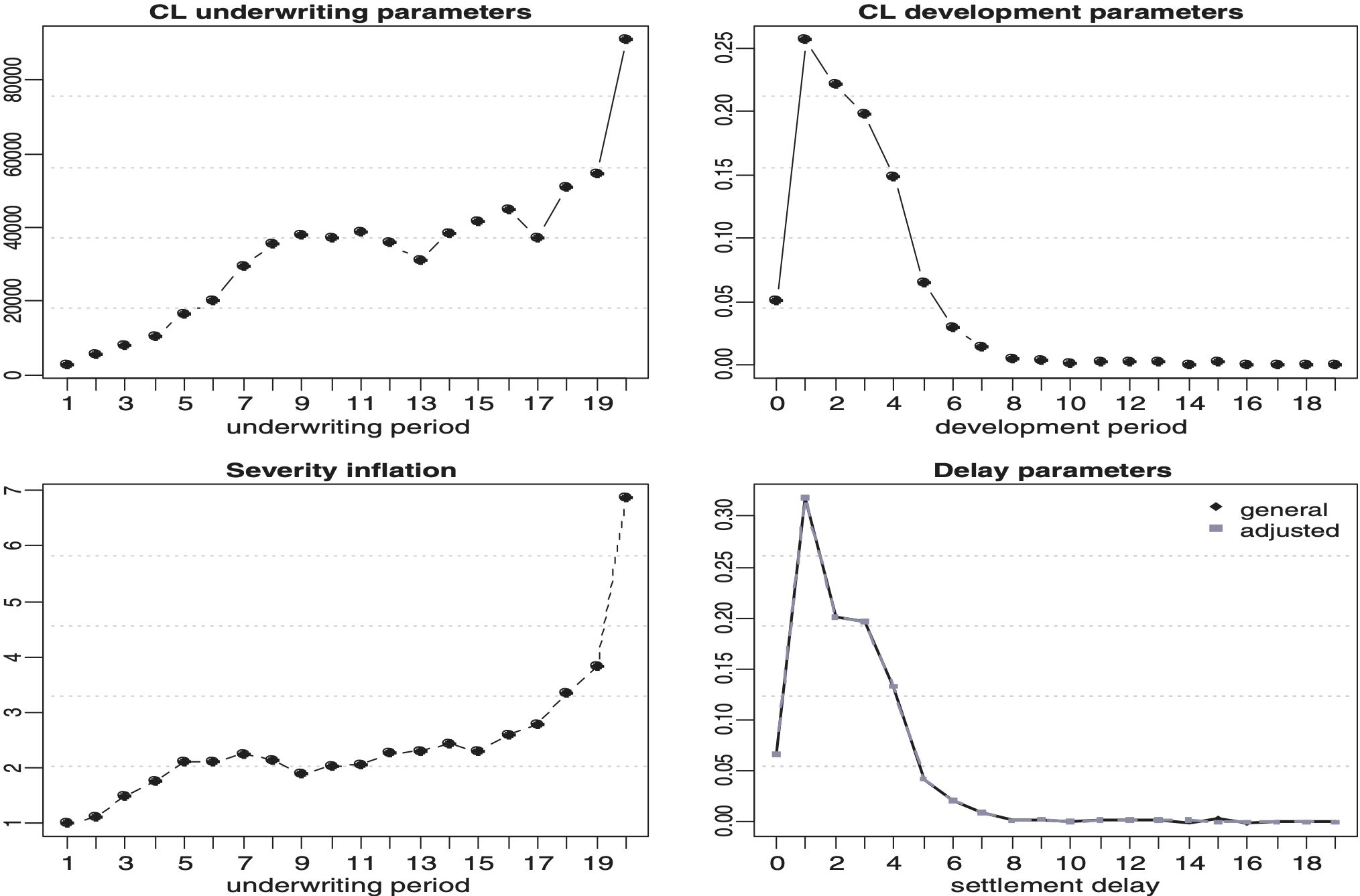
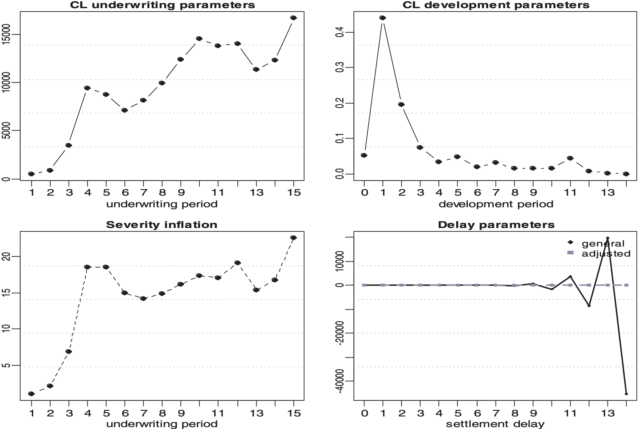
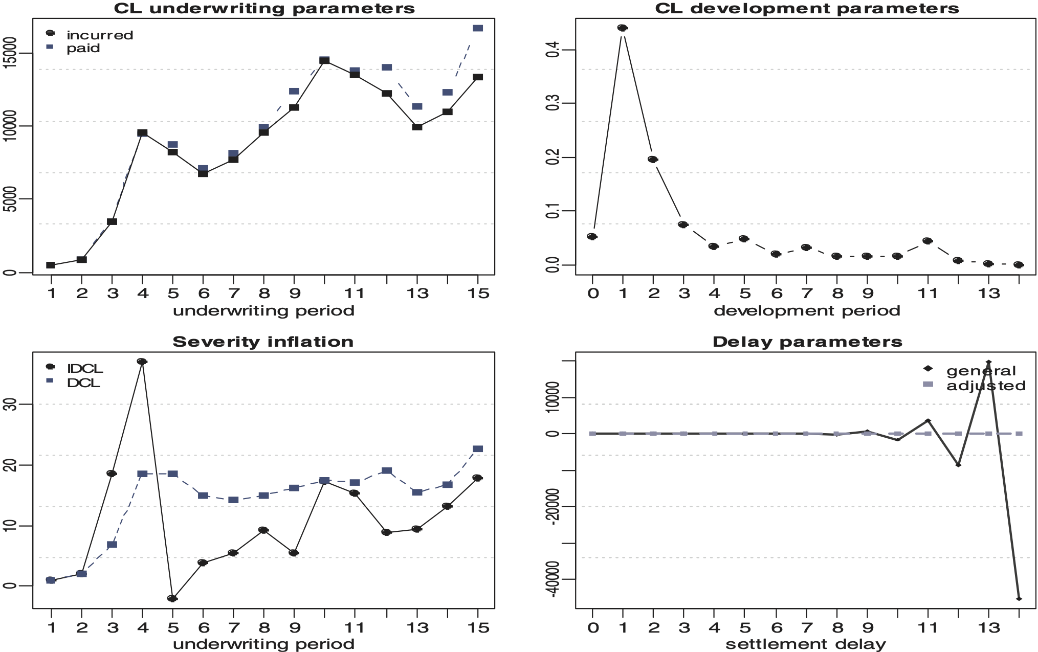
Table 1 shows the values of each parameter obtained by applying the DCL model to a motor personal injury (Motor BI) portfolio and on a motor fleet property damage (Motor PD) portfolio. Note that \(\hat{\alpha}_i\) and \(\hat{\beta}_j\) are obtained from the triangles of the claim numbers when DCL is applied. Figures 1 and 2 show the estimated chain ladder parameters, underwriting \(\hat{\tilde{\alpha}}_i\), development \(\hat{\tilde{\beta}}_j\), together with the estimates of severity inflation\(\hat{\gamma}_i^{D C L}\) and delay \(\hat{\pi}_k\) for the DCL method. Note that here the estimates of the chain ladder parameters are obtained from the triangles of aggregated amounts in order to make comparisons between the standard chain ladder estimates and the estimates from the models described in this paper.

Figure 1.Motor BI, chain ladder estimated parameters, underwriting \(\hat{\alpha}_i\) and development \(\hat{\beta}_j\), and DCL estimates of severity inflation \(\hat{\gamma}_i\) and delay \(\hat{\pi}_k\) (“general” refers to the solutions of the linear system described in Section 3.1 and “adjusted” refers to the adjusted values which are defined afterwards and denoted by \(\hat{\tilde{\pi}}_k\)).

Figure 2.Motor PD, chain ladder estimated parameters, underwriting \(\hat{\alpha}_i\) and development \(\hat{\beta}_j\), and DCL estimates of severity inflation \(\hat{\gamma}_i\) and delay \(\hat{\pi}_k\).

Each parameter has a different effect in explaining the reserve estimates. The underwriting year parameter estimate \(\hat{\alpha}_i\) is an increasing function of time. This is consistent with the expectation that the average cost per claims does increase year-on-year. However, we observe the well known unstable behavior in the most recent underwriting years. The development period parameter estimate \(\hat{\beta}_j\) peaks in the first development periods and then reduces smoothly afterwards because the development factors at that point are estimated from insufficient and potentially volatile data in the lower left corner of a run-off triangle. Also, most claims will have a high proportion of payment at those early development periods. The severity inflation parameter estimate \(\hat{\gamma}_i^{D C L}\) pattern is consistent with an underwriting or accident year effect similar to that of the parameter estimate \(\hat{\alpha}_i\) but also has the same weakness in the most recent years. The severity inflation on the Motor PD data exhibits an unusual and pronounced jump in the 4th development period which is likely to be independent from any actual claim experience. The delay parameter estimate \(\hat{\pi}_k\) patterns for the Motor BI has a development period effect spreading across a number of years. This is consistent with liability lines of business which normally take many years to settle. There appears to be no settlement delay in the Motor PD data. Again, this is consistent with property damage lines of business which are usually settled within a couple of months. Therefore there is no delay that could be measured on an annual scale except for the very immature data in the most recent accident years.

In the next subsection we will define another method to estimate the severity inflation parameter. It will be based on incurred data and aims to overcome the weakness of its DCL method estimate in the most recent underwriting years. However, note that this approach will not work for the underwriting parameter \(\alpha_i\) since it already uses incurred data.

3.2. The BDCL method

The CLM and Bornhuetter-Ferguson (BF) methods are among the easiest claim reserving methods, and due to their simplicity they are two of the most commonly used techniques in practice. Some recent papers on the BF method include Alai, Merz, and Wüthrich (2009, 2010), Mack (2008), Schmidt and Zocher (2008) and Verrall (2004). The BF method was introduced by Bornhuetter and Ferguson (1972) and aims to address one of the well-known weaknesses of CLM, which is the effect that outliers can have on the estimates of outstanding claims. To do this, the BF method incorporates prior knowledge from experts and is therefore more robust than the CLM method which relies completely on the data contained in the run-off triangle.

For the purpose of imitating BF, the BDCL method follows identical steps as DCL but instead of using the estimates of the very volatile inflation parameters \(\gamma_i\) from the triangle of paid claims, they are estimated using some extra information. The information arises from using the triangle of incurred claim amounts \(\Theta_m\). In this way, the BDCL method then consists of the following two-step procedure:

1. Step 1: Parameter estimation.

   Estimate the model parameters \(\alpha_i, \beta_j, \pi_k\) and \(\mu\) using DCL for the data in the triangles \(N_m\) and \(X_m\).

2. Step 2: BF adjustment.

   Repeat this estimation using DCL but replacing the triangle of paid claims with the triangle of incurred data: \(\Theta_m\). Keep only the resulting estimate of the inflation parameter and denote it by \(\hat{\gamma}_i^{B D C L}\)

After Steps 1 and 2, the parameter estimates are obtained: \(\left\{\hat{\alpha}_i, \hat{\beta}_j \hat{\mu}, \hat{\gamma}_i^{B D C L}, \hat{\pi}_k \mid k=0, \ldots, m-1, i=1, \ldots m,j=0, \ldots, m-1\right\}\). In general, it would be possible to use other sources of information from those suggested here. Thus, Step 2 could be defined in a more arbitrary way, thereby mimicking more closely what is often done when the BF technique is applied. In this way, the process described in this section could be viewed in a more general way.

Figure 3.Motor BI, BDCL estimated parameters, underwriting \(\alpha_i\) and development \(\beta_j\), and DCL estimates of severity inflation \(\gamma_i\) and delay \(\pi_k\).

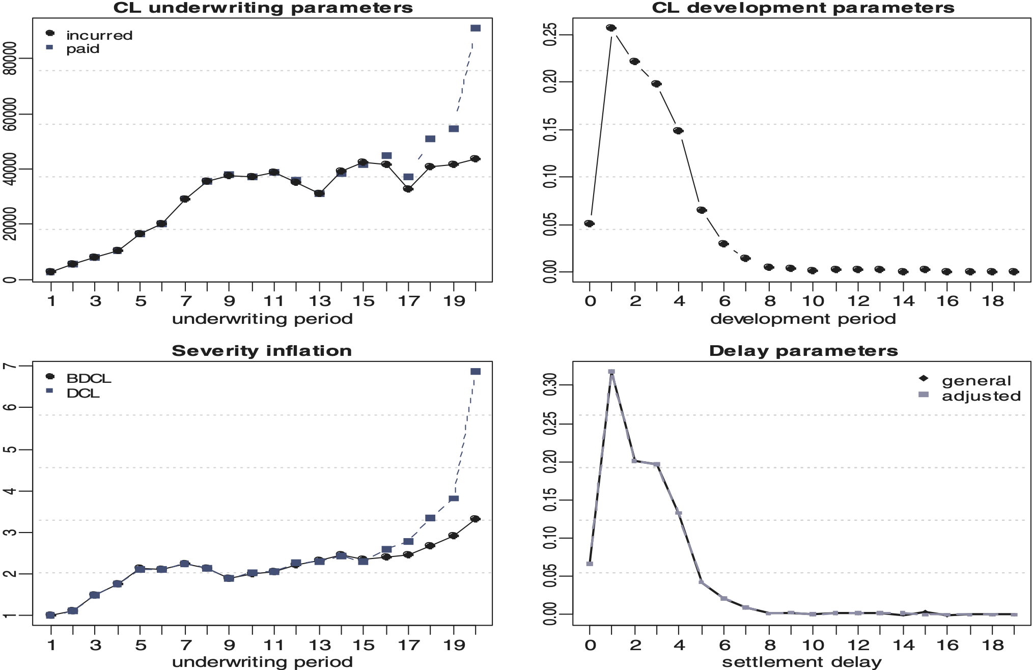
Figures 3 and 4 depict the estimated parameters, underwriting \(\hat{\alpha}_i\), development \(\hat{\beta}_j\), severity inflation \(\hat{\gamma}_i^{B D C L}\) and delay \(\hat{\pi}_k\) using BDCL. Note that in these figures and all future figures in this paper, the underwriting and development parameter estimates plotted are chosen so that a direct comparison can be made with the chain ladder parameter estimates. The aggregated payments triangle has very few information in the latest underwriting periods and is thus very volatile there. We see that the underwriting parameter estimate \(\hat{\alpha}_i\) derived from the aggregated incurred claim amounts triangle doesn’t have the unrealistic jump at the end of the period which is estimated by the aggregated payments triangle. This results in a more stable severity inflation parameter estimate \(\hat{\gamma}_i^{B D C L}\).

Figure 4.Motor PD, BDCL estimated parameters, underwriting \(\alpha_i\) and development \(\beta_j\), and DCL estimates of severity inflation \(\gamma_i\) and delay \(\pi_k\).

3.3. The IDCL method

In the BDCL definition, we introduced an additional triangle of incurred claims in order to produce a more stable estimate of the severity inflation \(\gamma_i\). The derived BDCL method is a variant of the BF technique using the prior knowledge contained in the incurred triangle. One natural question is whether the derived reserve is the classical incurred chain ladder estimate. Unfortunately, this is not the case and the BDCL method does not replicate the results obtained by applying the classical chain ladder method to the incurred triangle. Practitioners often regard the incurred reserve to be more realistic for many datasets compared to the classical paid chain ladder reserve. In this respect, we introduce in this section a new method to estimate the DCL model which completely replicates the chain ladder reserve from incurred data. It is simply defined just by rescaling the underwriting inflation parameter estimate from the DCL method. Specifically, we define a new scaled inflation factor estimate \(\hat{\gamma}_i^{I D C L}\) such that

\[ \hat{\gamma}_{i}^{D C L}=\frac{R_{i}^{*}}{R_{i}} \hat{\gamma}_{i}^{D C L}, \]

where \(\left(R_i, \hat{\gamma}_i^{D C L}\right)\) are the outstanding liabilities estimate for accident year i and the inflation parameter estimate respectively, using DCL (cf. Section 3.1), and \(R_i^*\) is the outstanding liabilities estimate for accident year i derived by the classical chain ladder method for incurred data. With the new inflation parameter \(\hat{\gamma}_i^{I D C L}\) (and keeping all other estimates as in DCL and BDCL) the accident year reserve completely replicates the CLM reserve estimates on the incurred triangle. Therefore, we call this method IDCL.

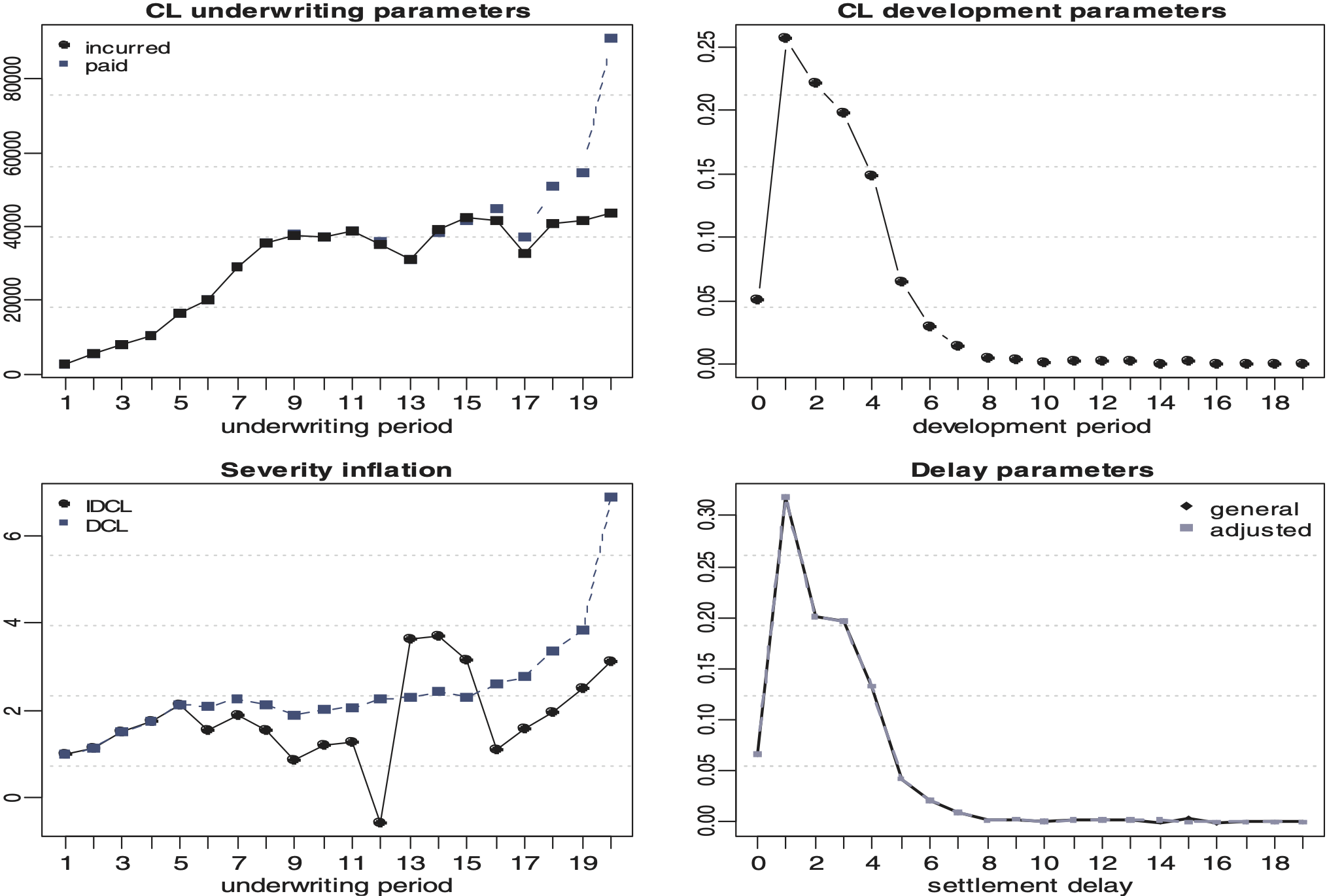
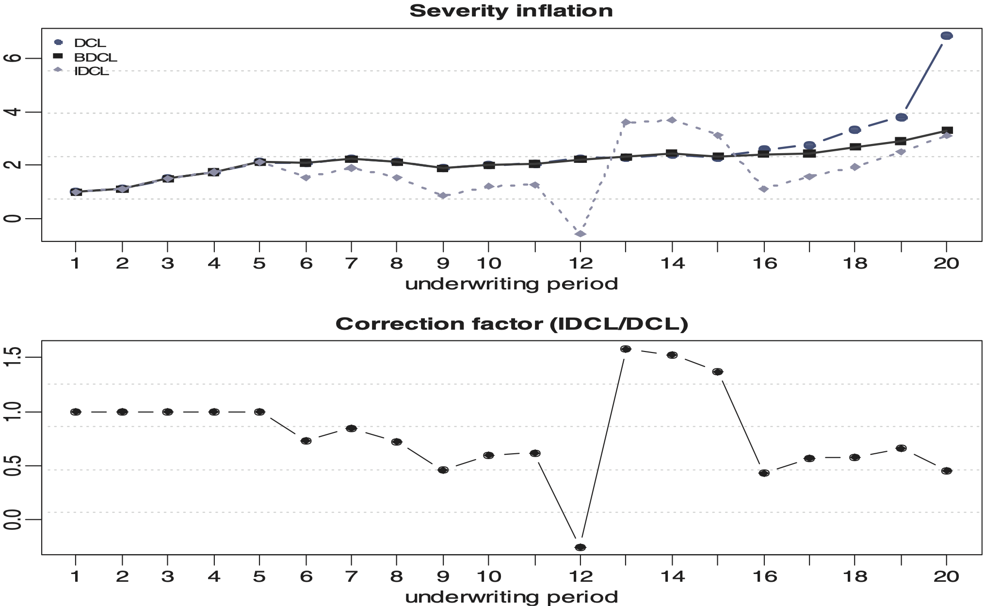
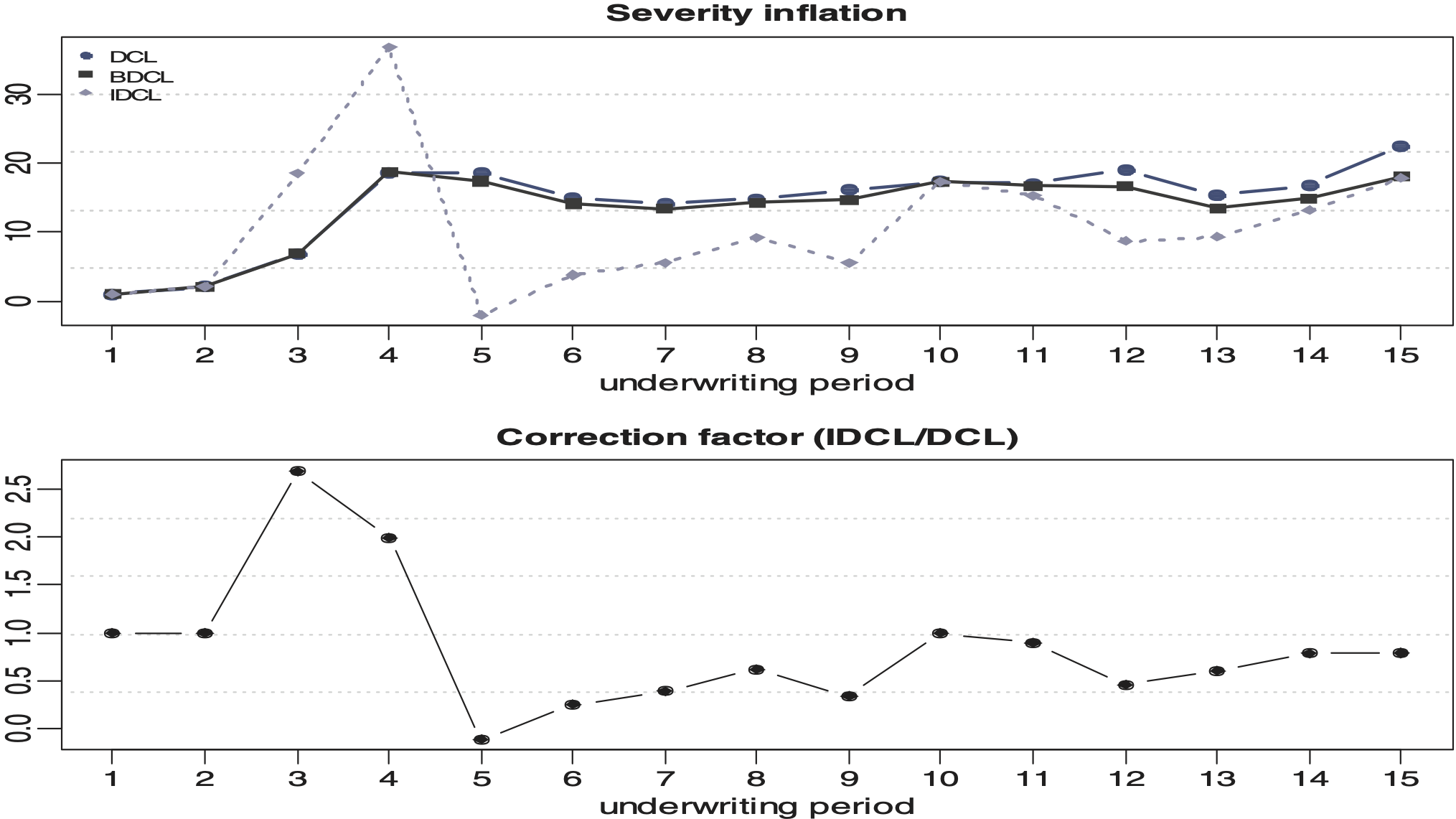
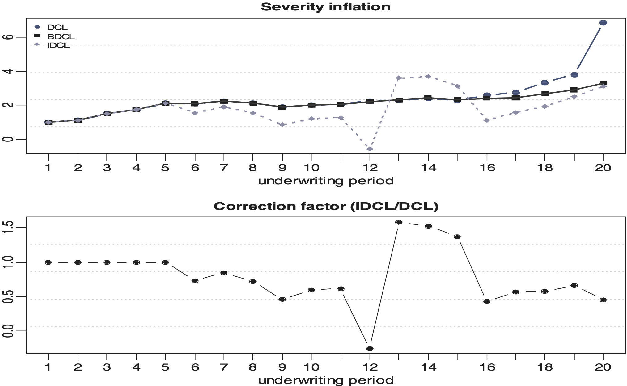
Figures 5 and 6 display the estimated parameters for both lines of business under the IDCL. Figures 7 and 8 illustrate the different severity inflation estimates. Table 2 shows the inflation parameter \(\gamma_i\) for each parameterisation, for each accident year, and for each line of business. The large value in accident year 2 is probably caused by a significant change in risk or a process review in the Motor PD portfolio. It appears that the book increased in size suddenly or that there has been a new claims management philosophy causing an artificial jump which is not consistent with the actual experience and therefore is unlikely to be repeated in the future. This shows that IDCL should not be applied naïvely. In practice, it would be advisable to remove such unusual event from the data or curtail the triangles to periods which are not affected by the rare event.

Figure 5.Motor BI, IDCL estimated parameters, underwriting \(\alpha_i\) and development \(\beta_j\), and DCL estimates of severity inflation \(\gamma_i\) and delay \(\pi_k\).

Figure 6.Motor PD, IDCL estimated parameters, underwriting \(\alpha_i\) and development \(\beta_j\), and DCL estimates of severity inflation \(\gamma_i\) and delay \(\pi_k\).

Figure 7.Motor BI, estimated inflation parameters for DCL, BDCL, and IDCL.

Figure 8.Motor PD, estimated inflation, parameters for DCL, BDCL, and IDCL.

4. Forecasting outstanding liabilities for RBNS and IBNR claims

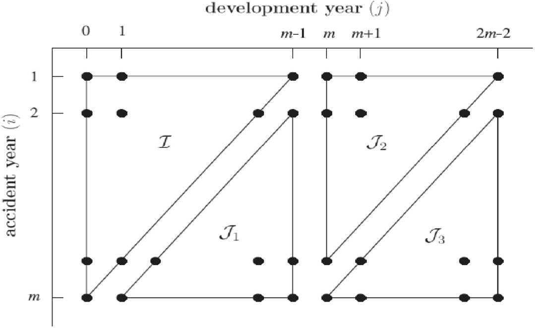
In the previous section we estimated all parameters of the double chain ladder model. In this section we will use these estimated parameters to calculate point forecasts of the RBNS and IBNR components of the outstanding liabilities. Using the notation of Verrall, Nielsen, and Jessen (2010) and Martínez-Miranda, Nielsen, and Verrall (2012), we consider predictions over the triangles illustrated in Figure 9 where

\[ \begin{aligned} J_{1} & =\left\{\begin{array}{l} i=2, \ldots, m ; j=0, \ldots, m-1 \\ \text { so } i+j=m+1, \ldots, 2 m-1 \end{array}\right\}, \\ J_{2} & =\left\{\begin{array}{l} i=2, \ldots, m ; j=0, \ldots, 2 m-1 \\ s o i+j=m+1, \ldots, 2 m-1 \end{array}\right\}, \\ J_{3} & =\left\{\begin{array}{l} i=2, \ldots, m ; j=0, \ldots, m-1 \\ \text { so } i+j=3 m+1, \ldots, 3 m-1 \end{array}\right\} . \end{aligned} \]

Then, we define the RBNS reserve as

\[ \hat{X}_{i j}^{R B N S}=\sum_{l=i-m+j}^{j} N_{i, j-l} \hat{\pi}_{l} \hat{\mu} \hat{\gamma}_{i}, \]

where \((i, j) \in J_1 \cup J_2\). The IBNR reserve component is

\[ \hat{X}_{i j}^{1 B N R}=\sum_{i=0}^{i-m+1-1} \hat{N}_{i, j-l} \hat{\pi_{l}} \hat{\mu} \hat{\gamma}_{l}, \]

where \(\hat{N}_{i j}=\hat{\alpha}_i \hat{\beta}_j\) and \((i, j) \in J_1 \cup J_2 \cup J_3\).

Figure 9.Index sets for aggregate claims data, assuming a maximum delay \(m - 1\).

Note that the RBNS and the IBNR component differ in how the numbers of incurred claims are handled. In the RBNS component the number of incurred claims is known and thus used. In the IBNR component, that is not the case and we have to deal with estimates. However, if we replace the known number of the incurred claims in the RBNS component by its estimates, i.e., we define the RBNS component as

\[ \hat{X}_{i j}^{R B N S(C L M)}=\sum_{l=i-m+j}^{j} \hat{N}_{i, j-l} \hat{\pi} \hat{\mu}_{l} \hat{\gamma}_{i}^{D C L}, \]

where \(\hat{N}_{i j}=\hat{\alpha}_i \hat{\beta}_j\), DCL would completely replicate the results achieved by the classical CLM. In other words \(\hat{X}_{i j}^{R B N S(C L M)}+\hat{X}_{i j}^{I B N R}\) are exactly the point estimates of the classical CLM on the cumulative payments triangle \(A_{i j}=\sum_{k=1}^j X_{i k}\). Also, note that the classical CLM would produce forecasts over only \(J_1\). If the classical CLM is being used, it is therefore necessary to construct tail factors in some way. For example, this is sometimes done by assuming that the run-off will follow a set shape, thereby making it possible to extrapolate the development factors. In contrast, DCL also provides the tail over \(J_2 \cup J_3\) using the same underlying assumptions about the development. Thus, DCL is consistent over all parts of the data, and it uses the same assumptions concerning the delay mechanisms producing the data throughout.

Table 3 shows the RBNS and IBNR reserve and also the total (RBNS + IBNR) forecasts split by accident year for Motor BI. Table 4 shows the same reserves for Motor PD. As a benchmark for comparison purposes, the predicted reserves on the classical CLM are also shown in the last two columns of both tables.

All four methods predict a large amount of negative RBNS for the Motor PD. The negative amounts are ultimately balanced against the IBNR to give “reasonable” total reserve. The negative values for RBNS are due to large amount of recoveries in the incurred triangles, i.e., the model is picking up the uncertainty around the case estimates and using it to predict the results. A possible solution for avoiding such inconsistency is to remove the recoveries from the triangles, run the model on the claims amounts net of recoveries, rerun the same model on the recoveries only and then add back both results to obtain a more realistic reserve cash flow. Unfortunately, in practice, triangles net of recoveries are not readily available. A more sophisticated model will have to be developed to manage any occurrence of negative claims as well as their magnitude if such adjustment is not allowed.

5. Model validation

This section describes the validation strategy used to decide which method should be used among the DCL, BDCL and IDCL methods discussed in Section 3. Section 5.1 acknowledges the potential impact of the development factors (cf. Section 3.1) on the model output and checks for any additional improvement gained by limiting the data used to estimate the model to recent calendar years only. Section 5.2 provides details of the validation procedure which is based on back testing.

5.1. Estimating forward development factors

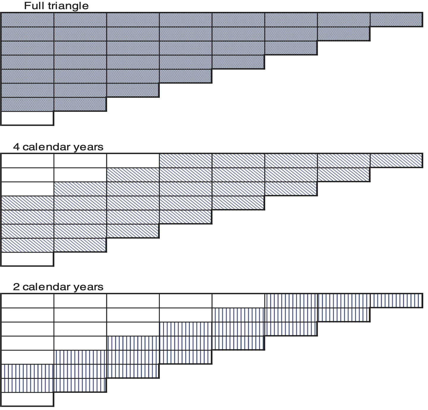
Using larger amounts of data should intuitively reduce the volatility and improve a model’s predictive power. However, since the triangles are from actual data over 20 years, the emergence of claims, settlement delay and amount paid in recent years might not be consistent with those at the beginning of the period. This can be illustrated by comparing parameter estimates using different portions of the data. We will estimate the development factors with five different datasets which differ in the amount of data used. The biggest dataset will contain the full data, that is, the cumulative aggregated payments triangle \(A_{i j}=\sum_{k=1}^j X_{i k}\). The other four datasets will contain entries only of the five to two most recent calendar years (cf. Figure 12).

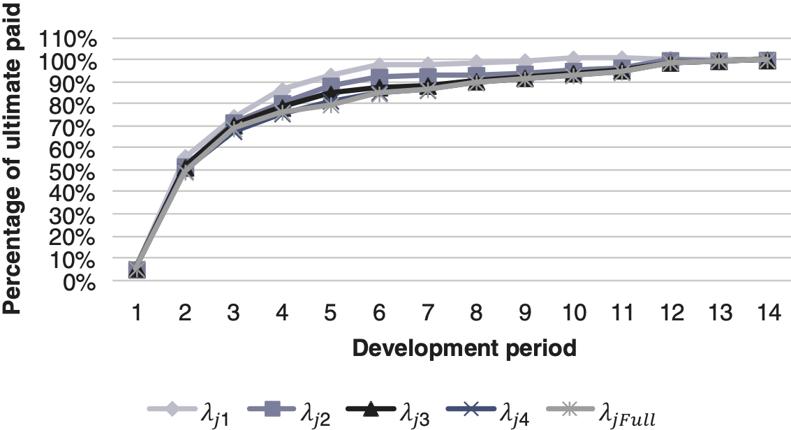
Table 5 shows the development factors \(\lambda_j\) with respect to the number of calendar years used to generate them. For example, \(\lambda_{j \text { Full }}\) uses the full triangle. It should be noted that using an increasing number of calendar years makes the \(\lambda_j\) steeper because of the difference in the average claim paid between the two ends of the calendar year period. This is caused by year-on-year severity inflation. Figures 10 and 11 show the expected cumulative proportion of claims settled based on the calendar year period used to derive the \(\lambda_j\). Note, the cumulative proportion of claims settled \(\Lambda_j\) is calculated by

\[ \Lambda_{j}=\frac{1}{\prod_{j}^{m} \lambda_{j}} \]

Figure 10.Motor BI settlement pattern.

Figure 11.Motor PD settlement pattern.

5.2. Back testing and robustness

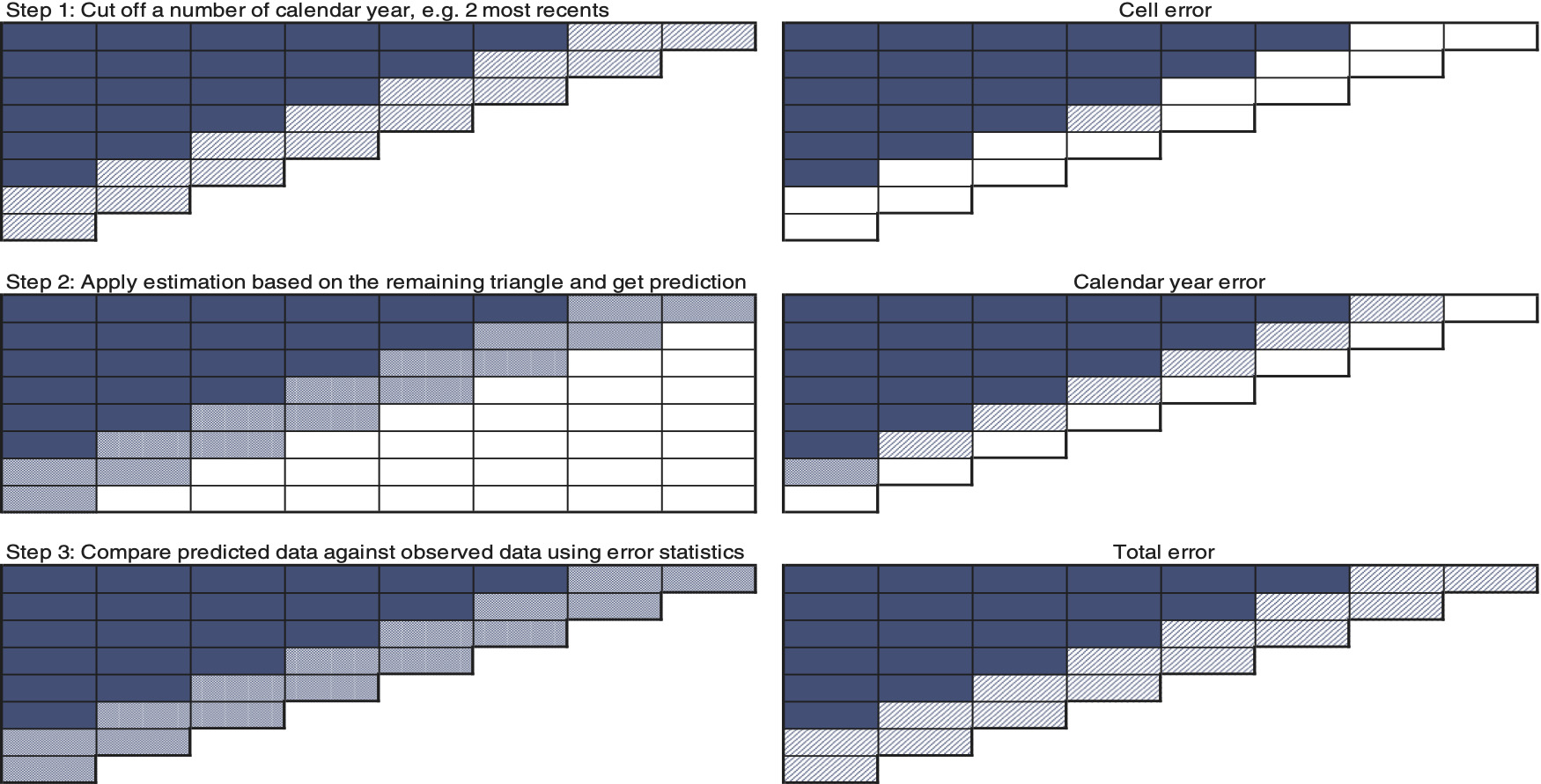
The underlying process is based on back testing data previously omitted while estimating the parameters for each method. The validation process will be based on the Motor BI data which appear to be free from operational issues. Furthermore, we will also run the back testing by limiting the data of the cumulative triangles which are older than two or four calendar years, respectively (cf. section 5.1 and Figure 12). The three statistics defined below are used to assess the prediction errors within a cell, a calendar year or across the total segment removed from the triangle. The full process is illustrated in Figure 13. Let \(\hat{X}_{i j}\) be the estimated cell entry and let \(X_{i j}\) be the omitted data. Then we define

Figure 12.Calendar years used for development factors.

Figure 13.Back testing and prediction errors.

1. Cell error:

   \[ \sqrt{\frac{\sum_{i j}\left(X_{i j}-\hat{X}_{i j}\right)^{2}}{\sum_{i j} X_{i j}^{2}}} \]

2. Calendar year error:

   \[ \sqrt{\frac{\sum_{i}\left(\sum_{1} X_{i j}-\hat{X}_{i j}\right)^{2}}{\sum_{i}\left(\sum_{j} X_{i j}\right)^{2}}} \]

3. Total error:

   \[ \left\lvert\, \frac{\sum_{i j} X_{i j}-\hat{X}_{i j}}{\sum_{i j} X_{i j}}\right. \]

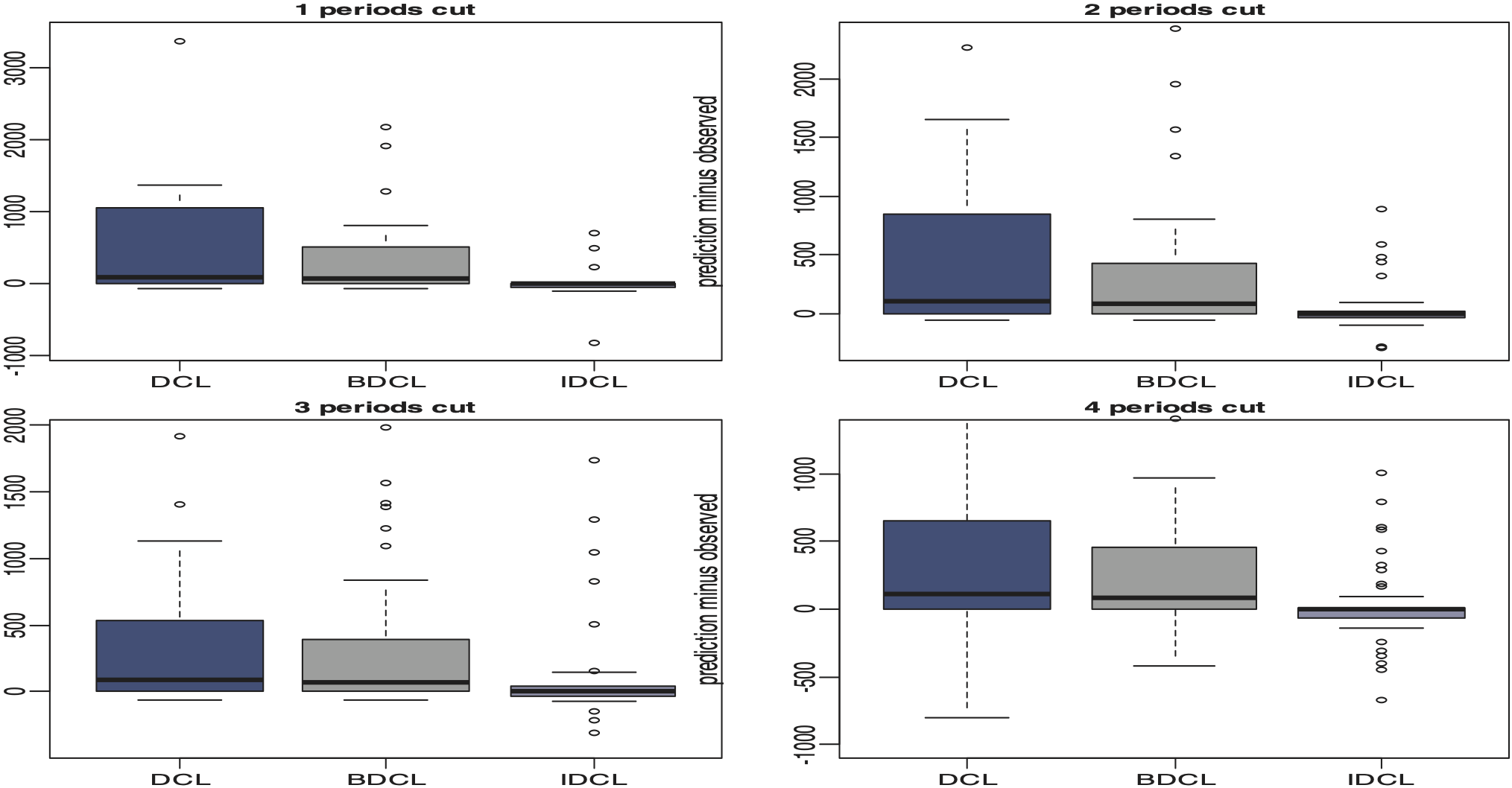
In Table 6, the first column describes the number of previous calendar years used to calculate the development factors. The second column lists the number of calendar years removed to perform the back testing. A lower percentage error suggests a better prediction. It appears that the DCL method is almost always the weakest with for example, up to a 95.97% by cell error on one period of back testing when four calendar years are used to estimate the parameters. The BDCL seems stronger than IDCL on longer period of back testing especially when more data are used. However, the IDCL generally outperforms the other methods. Figure 14 confirms that the BDCL is more stable than the DCL and the IDCL generally stronger than the BDCL.

Figure 14.Box plot of the DCL, BDCL and IDCL cell error quartiles.

6. Conclusions

In this paper, three different types of estimation methods were considered. The DCL formalizes the classical CLM mathematically by setting the implicit factors, explicitly. However, since the DCL method is performed only on triangles of claims count and paid claims, excessive volatility in the prediction of the most recent accident year’s reserves can be introduced as shown in Figures 1 and 2. The instability of the severity inflation parameter estimation can be resolved by the introduction of the BDCL method. As expected, the BDCL predictions are less volatile than those of the DCL as shown in Table 2. Once working with the incurred claim amounts triangle we were also able to replicate the classical chain ladder point estimates on incurred data. The user would intuitively question the variability between estimates from the three methods. The purpose of the reserving exercise should dictate the most relevant method to select. For instance, using the DCL for regulatory purposes where prudence is the norm and using the BDCL or IDCL for internal management accounts reporting when realistic figures are more suited. The validation showed that BDCL and IDCL are superior to DCL. However, the validation was not able to distinguish clearly between BDCL and IDCL. For the sake of argument, we applied the DCL model on two separate datasets to assess how robust the model is to incorrect or erroneous data and we obtained very different intermediate results but overall reasonably correct final reserve. The IDCL would be preferred for short-tail lines of business, e.g., property damage which will be less affected by severity inflation whilst the BDCL would be preferred for long-tail classes such as liability. An alternative to the methods discussed above is a double chain ladder model with a severity inflation parameter having a calendar year dependency, modelled by a time series with a deterministic drift and a stochastic volatility. But this is beyond the scope of this paper and might be subject of further research.