
1. Introduction
There is a growing body of scientific evidence that extreme weather events are increasing in frequency and intensity (Intergovernmental Panel on Climate Change 2014a). This phenomenon has already led to significant property damages and mounting insurance losses due to floods, storms, hurricanes, and other natural disasters (e.g., see Bouvet and Kirjanas 2016; LSE (London School of Economics and Political Science) 2015; NAIC 2016; Smith and Matthews 2015 and references therein). To mitigate the adverse effects of this upward trend, insurers need a comprehensive attribution analysis of climate-related claim dynamics at a local level and a reliable quantification of future climate-related risks.
Whereas a vast literature exists on modeling insurance risks due to weather disasters and catastrophic events (see, e.g., overviews by Grossi, Kunreuther, and Windeler 2005; Kunreuther and Michel-Kerjan 2012; Toumi and Restell 2014), little is known about how to address risks due to less extreme events, the so-called low individual but high cumulative impact events, which have exhibited rising frequencies over time. The yet-scarce literature on this topic primarily focuses on modeling a number of weather-related insurance claims (Scheel et al. 2013; Soliman et al. 2015; Lyubchich and Gel 2017) rather than on the dynamics of related losses. A few recent studies on predicting insurance losses due to extreme but noncatastrophic weather events include Haug et al. (2011), who consider Norwegian home insurance data aggregated at a provincial level; Cheng et al. (2012), who analyze rainfall-related damage in four cities in Ontario, Canada; and Held et al. (2013), who use various downscaling methods to evaluate winter-storm-induced residential losses in Germany.
In this paper, we develop an attribution analysis of weather-related insurance losses on a daily scale and present a comprehensive statistical methodology for assessing future loss dynamics. Our study also provides a valuable insight into uncertainties of the developed forecasts for claim severities with respect to various climate model projections and greenhouse emission scenarios. While the current paper is only one of the very first steps on the path of a systematic and sound analysis of future insurance risk due to noncatastrophic weather events, the results of our study pave the way for more accurate short- and long-term cost-benefit assessment of climate adaptation in the insurance sector.
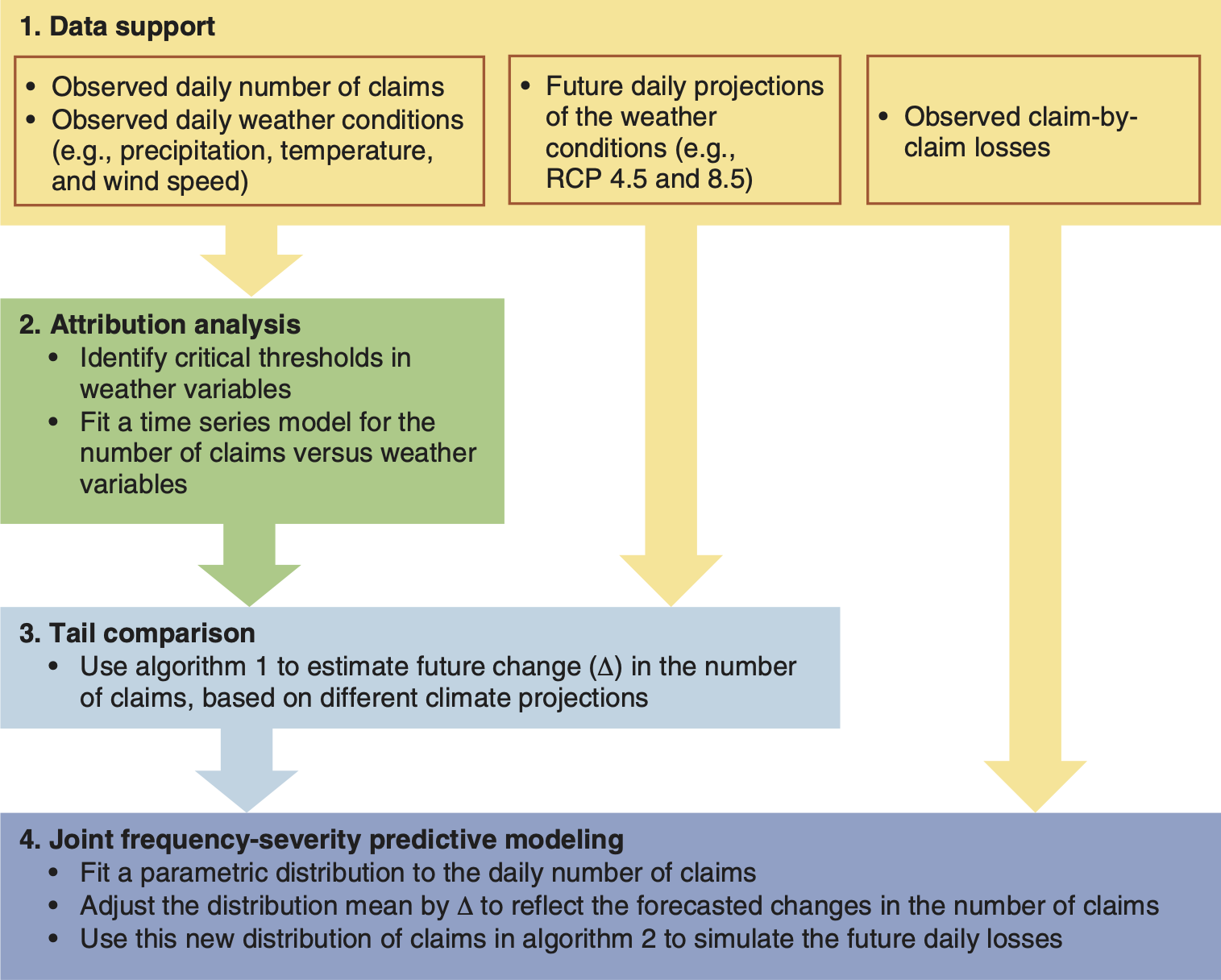
The strategy we employ includes an analysis of nonlinear dependencies between weather and claims data; detection of critical thresholds, or tipping points leading to an increased number of claims; and joint frequency-severity predictive modeling of weather-related daily losses. A summary of the proposed analysis strategy is presented in Figure 1.1; all the details are explained further in the paper.

The remainder of this paper is organized as follows. Section 2 describes the data: recorded insurance claims and weather conditions as well as climate projections (Step 1 in Figure 1.1). Section 3 showcases the methods of attribution analysis and tail comparison (Steps 2 and 3 in Figure 1.1). Section 4 presents joint frequency-severity predictive modeling and forecasts (Step 4 in Figure 1.1). The paper is concluded with a discussion in Section 5.
2. Data
In this study, we use Canadian residential insurance claim data, local weather station data, gridded instrumental data products, and regional climate model data that are described below.
Insurance Data The insurance data consist of redacted, anonymized, and aggregated home insurance claims (counts and dollar losses) incurred due to weather damage reported by postal code during 10 years spanning 2002 to 2011. The data have been internally validated for quality control, and the selected geographic locations represent four urban areas in Canada, which we call City A, City B, City C, and City D. City A is situated in the continental climate zone in the high prairie, City B directly on a lake in the Great Lakes area, City C in eastern Canada with cold and temperate continental climate characterized by four distinct seasons, and City D in eastern Canada with a similar hemiboreal climate with no dry season but at double the elevation of City C. All four selected cities are medium sized and have similar population densities. At the preprocessing stage, we normalize the daily number of claims by the number of policyholders on each day and adjust the dollar amounts by the metropolitan area composite quarterly index of apartment building construction (Table 327-0044, http://www5.statcan.gc.ca [page no longer available]). Since we have no data on collected premiums and thus are unable to evaluate the loss ratios, similarly to Frees, Meyers, and Cummings (2012), we focus on the assessment of claim frequencies and severities (see Frees, Derrig, and Meyers 2014 for a detailed discussion and literature overview).
Weather Observations The weather observations we use in our analysis are provided by Environment Canada in its Digital Archive of Canadian Climatological Data and are available from http://climate.weather.gc.ca/. Daily climatological data are obtained for each city, from which we use mean temperature, total precipitation (millimeters, snow is converted to water equivalents), and speed of maximum gust (kilometers per hour) for our analyses. Gust speeds less than 31 kilometers per hour (8.6 meters per second) are not reported, but this is well below the wind level that would be expected to cause damage claims (Stewart 2003).
Climate Model Output Data from three climate model experiments used in this study are derived from the CanRCM4 version of the Canadian Regional Climate Model run by the Canadian Center for Climate Modeling and Analysis. The model is described in Scinocca et al. (2016), and the model experiments used here were part of the North American Coordinated Regional Climate Downscaling Experiment (Giorgi and Gutowski 2015). Regional climate models require lower-resolution input data from either processed observational datasets or a global-scale climate model.
To evaluate uncertainty due to various scenarios of global warming, we use available data at 25 kilometers (0.22 degree) spatial resolution from two CanRCM4 experiments run with the second-generation Canadian Earth System Model, CanESM2, as input data. In particular, we consider two runs from 2006 to 2100, forced with greenhouse gas scenarios known as RCP 4.5 and RCP 8.5. These Representative Concentration Pathways (RCPs) are commissioned by the IPCC and have been used widely in different efforts to study potential impacts of climate change. The RCP 4.5 scenario stabilizes greenhouse forcing to 4.5 watts per square meter before 2100 and represents a world where greenhouse gas emissions are brought under control by a variety of human actions. RCP 8.5 is a business-as-usual scenario where greenhouse gas forcing from human activities is not curtailed and rises to 8.5 watts per square meter by 2100. The climate in each of the model runs develops independently, so small differences between model runs are expected due to normal stochastic noise in the climate system.
In addition, to assess uncertainty due to the potential discrepancy between climate model output and weather observations, we consider a third experiment of the CanRCM4 regional model that was run for 1989 to 2009 with ERA-Interim reanalysis data (Dee et al. 2011) as input data. A climate reanalysis provides an estimate of the state of the climate system over the whole globe based on observations by coupling models with the observations. Like global climate model output, reanalysis data are continuous (unlike true observations) and can be used as the input data for the regional climate model. The ERA-Interim run of CanRCP4 represents a validation experiment to test how well the model represents the real world when the boundary condition inputs are from the real world rather than a model simulation.
3. Methods
To develop an attribution analysis of current weather-related losses and to assess dynamics of future claim severities, we combine the approaches of Soliman et al. (2015) and Lyubchich and Gel (2017) to modeling a number of weather-related claims, with a collective risk model (CRM) simulation algorithm of Meyers, Klinker, and Lalonde (2003). As a result, we propose a new method for joint frequency-severity predictive modeling of weather-related claim severities.
3.1. Triggering thresholds and attribution analysis
The first step of our methodology is to find critical thresholds for weather variables after which the severity of daily claims starts to increase monotonically (Lyubchich and Gel 2017). This knowledge of the weather effects is useful and important not only for accommodating nonlinearities in statistical models but also for the insurance industry to (1) dispatch insurance inspectors more efficiently (short-term), (2) establish appropriate building guidelines (long-term), and (3) formulate mitigation and prevention policies (long-term).
We use two methods to find the thresholds for observed insurance claim counts versus precipitation and wind speed: Classification and Regression Trees (Breiman et al. 1984; Derrig and Francis 2006; Hadidi 2003) and Alternating Conditional Expectations (ACE) transformations (Breiman and Friedman 1985). In addition to precipitation and wind speed, we considered a set of other atmospheric variables as potential predictors, including surface air temperature and pressure. However, our model selection analysis based on the Akaike information criterion (AIC) indicated that surface air temperature and pressure are not important predictors. (AIC is a model selection criterion that is widely used in numerous actuarial applications; see Brockett 1991; Frees, Derrig, and Meyers 2014; and references therein.)
The key ideas of Classification and Regression Trees (Breiman et al. 1984) are to
-
use piecewise constant functions to approximate nonlinear relationship between covariates (weather events) and a response variable (the number of house insurance claims due to adverse weather);
-
partition the predictor space with binary splits formulated in terms of the covariates, for example, identify thresholds in precipitation amounts that iteratively split the range for this variable into intervals; and
-
divide the whole domain into relatively homogeneous subdomains so the thresholds are chosen to provide the most homogeneous responses (claim counts) within each subdomain.
The tree-based models do not aim to construct an explicit global linear model for prediction or interpretation. Instead, the nonparametric tree-based approaches bifurcate the data recursively at critical points of covariates to split the data into groups that are as homogeneous as possible within and as heterogeneous as possible in between.
ACE is a nonparametric procedure that smoothly transforms predictors Xj to maximize the correlation between the response Y and transformed predictors fj(Xj) in a linear additive model (Breiman and Friedman 1985):
Y=α+k∑j=1fj(Xj)+ϵ,
where α is the intercept, fj(•) are some smooth nonlinear functions, k is the number of predictors, and ε are independent and identically distributed random variables. ACE also can employ a smooth transformation of response, that is, θ(Y), with the goal to minimize
E{θ(Y)−k∑j=1fj(Xj)}2
ACE transformations are splines with a predefined degree of smoothness, which is a special case of the generalized additive models (see Frees, Derrig, and Meyers 2014 for an overview of generalized additive models in actuarial sciences). In addition, a user can define such conditions as monotonicity and periodicity. In our analysis, we apply monotonic transformations to predictors without transforming the response.
Similar to Soliman et al. (2015) and Lyubchich and Gel (2017), we identify the thresholds from ACE transformation plots as the location of a breakpoint, which separates values of a weather predictor with trivial or no impact on the claim counts from the values having a significant impact. We finally truncate the weather predictors by setting the observations below selected thresholds to zero.
For the attribution analysis, we use a Generalized Autoregressive Moving Average (GARMA) approach by Benjamin, Rigby, and Stasinopoulos (2003), which accommodates integer-valued time series as well as non-Gaussianity of the variables. Let Y1, . . . , Yt be observed daily number of claims and Xt be a matrix of some exogenous regressors (precipitation, wind speed, etc.). Then, we can model conditional mean of Yt, given Y1, . . . , Yt − 1, X1, . . . , Xt, as
g(μt)=α+X′tβ+p∑j=1ϕj{g(Yt−j)−X′t−jβ}+q∑j=1θj{g(Yt−j)−g(μt−j)},
where g(•) is an appropriate link function, β is the vector of regression coefficients, φ are coefficients of the autoregressive part of order p, and θ are coefficients of the moving average part of order q. We use a zero-adjusted Poisson distribution to model daily claims, and link function g(•) is ln(•). See Cameron and Trivedi (2013); Creal, Koopman, and Lucas (2013); Fokianos (2015); and references therein for discussion of GARMA and other models for time series of counts.
The ACE-selected thresholds for precipitation and wind speed are reported in Table 3.1, along with the modeling results of the number of claims versus the weather predictors in GARMA(p, q) framework (3.1), where model order q was selected using AIC. The variability of estimated parameters is not high, and City B has generally higher βs, implying higher vulnerability to severe weather, which may be related to the city’s location directly in the Great Lakes area.
Remark Atmospheric thresholds that are currently adopted in civil engineering for building codes and standards primarily target extreme catastrophic events (see, e.g., Crawford and Seidel 2013; Gillespie, Antes, and Donnelly 2016; Obama 2015) and do not account for low individual but high cumulative impact events, which have exhibited rising frequencies over time but still remain a gray zone for risk management in the public sector. Hence, the burden of handling the outcomes of such low individual but high cumulative impact events is still on insurers and their clients. The study proposed here allows us to shed light on the critical thresholds and methods to derive them that could be used by the insurance companies to mitigate risks and minimize their losses—before the public-sector entities recognize the challenges of the gray zone of low individual but high cumulative impact events.
3.2. Adaptive extrapolation of claim frequencies
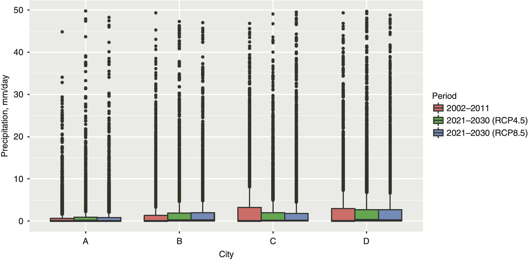
The selected thresholds and estimated model parameters further play a role in assessing future trends in the number of insurance claims. We obtain future values of atmospheric variables at daily resolution from the climate model projections. Similar to the modeling step (Section 3.1), we focus on the distribution tails above certain thresholds, which are both most important in insurance claims modeling and most dynamic as they exhibit greater changes than the rest of the distribution (Figure 3.1). Algorithm 1, which is a multivariate extension of the quantile-based method of Soliman et al. (2015), is based on the idea of numerical integration and allows us to naturally compare tails of two distributions (e.g., observed and forecasted precipitation) and use this information together with GARMA output to incorporate the climate change effects into claims forecasts.

We now apply Algorithm 1 to the claim dynamics in four cities and summarize our findings in Table 3.2. In particular, Table 3.2 suggests that claim counts will likely increase in all four cities during 2021–2030. The major increase is expected for City B, which is directly on a lake, indicating that changes in lake-derived moisture and its representation in the model should be explored in detail to fully understand this result. In general, higher elevation corresponds to a smaller increase in claim counts, but it is uncertain whether this is due to a reduced change in climate with elevation or is simply an artifact of the model representation of elevation and its dynamical impacts. There is not a large difference between the two scenarios for this time period because the climate projections do not diverge enough by 2021–2030 to make a substantial difference in the analysis. The small differences of a few percentage points between scenarios are likely due to climate system noise expected between different model runs.
3.3. Future projections with respect to different climate comparison scenarios
We now conduct an extensive study to examine the discrepancies arising from using different climate model outputs and observations. Specifically, our previously discussed analysis was based on weather observations in 2002–2011, and future projections have been based on comparing future climate model output against the weather observations.
To evaluate the uncertainty due to climate model projections and model discrepancies in estimating the “true” state of atmosphere, here we use an alternative to weather observations—output of the same climate model produced during an evaluation run for the recent past (1989–2009), which was forced with ERA-Interim reanalysis data. This analysis allows us to compare outputs of a climate model representation of the recent past and of the future (climate scenarios RCP 4.5 and RCP 8.5) at the same space-time resolution, to evaluate discrepancies in our analysis that arise due to differences between the climate model output and real-world observations. A disadvantage of using ERA-Interim forced output is the lack of model output data for certain years and varying data availability for different climate models. In our case, evaluations continued up to 2009, whereas available insurance data cover 2002–2011; thus, we had to reduce the period of analysis from 10 to 8 years: 2002 to 2009.
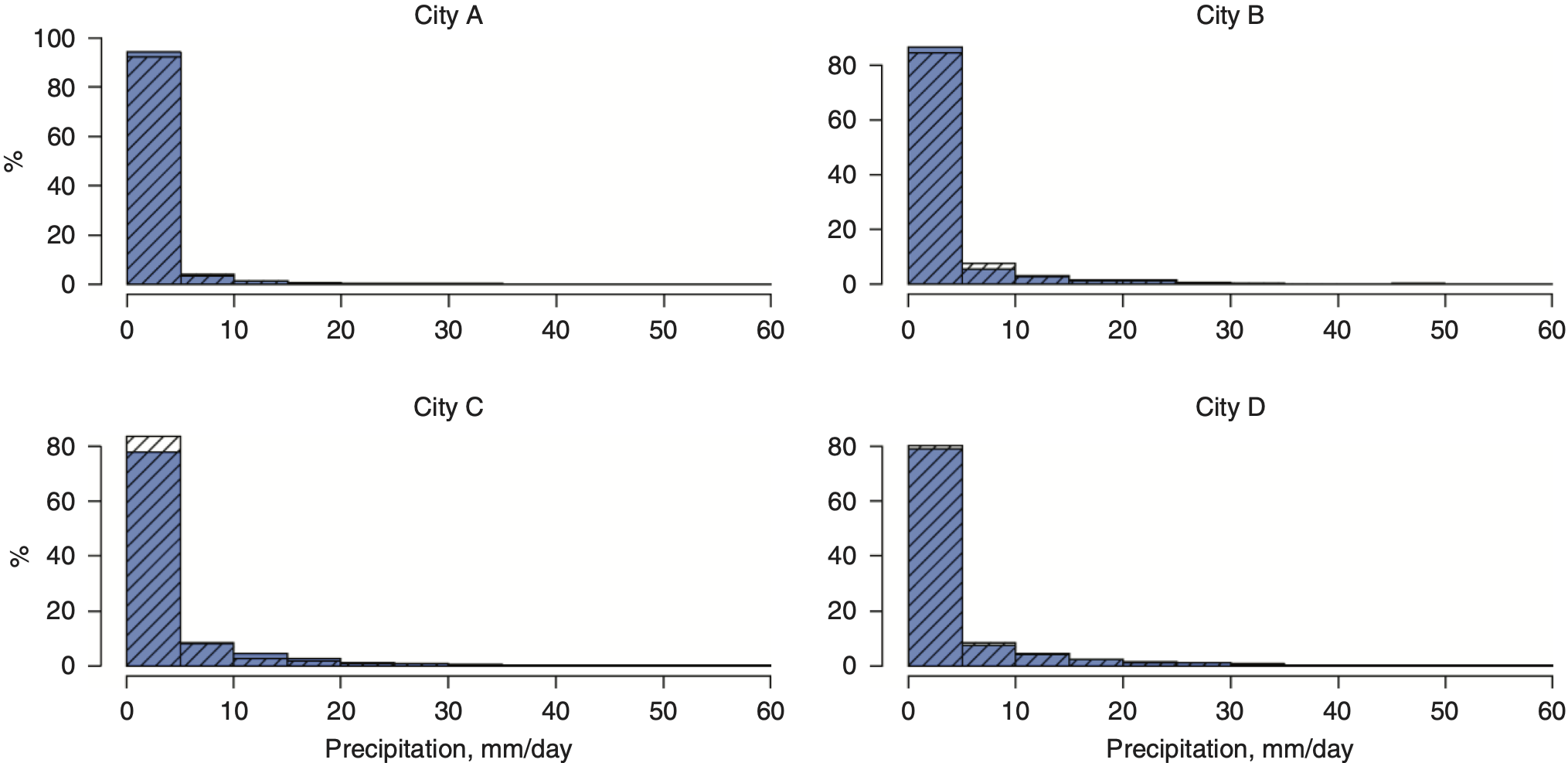
The climate model adequately represents the variables of the climate system that are important for our analysis. The model data are characterized by a higher proportion of days with very low precipitation (Figure 3.2), which is compensated for by higher extremes, such that the centers of the distributions, that is, the first to third quartiles, remain close to each other (Table 3.3).
_daily_precipitation_and_output_of_the_era-inte.png)
The projected numbers of weather-related home insurance claims were compared between three possible analysis scenarios summarized in Table 3.4. The scenarios differ based on (1) which weather data source (observations or climate model output) we use for estimating critical thresholds and GARMA modeling and (2) whether we compare future climate model output with the model itself (ERA-Interim evaluations) or with the observed data.
Scenario 1. Model number of claims (ncl) as a function of observed data (obs), that is, ncl ∼ b1 × obs. Compare tails of future climate projections with observed data and estimate the change δ1. The projected change in a future number of claims Δ is a function of b1 × δ1.
Scenario 2. Model number of claims (ncl) as a function of the reanalysis data (era), that is, ncl ∼ b2 × era. Compare tails of future climate projections with era and estimate the change δ2. The projected change in a future number of claims Δ is a function of b2 × δ2.
Scenario 3. Model number of claims (ncl) as a function of observed data (obs), that is, ncl ∼ b1 × obs. Compare tails of future climate projections with era and estimate the change δ2. The projected change in a future number of claims Δ is a function of b1 × δ2.
Remarkably, all three comparison scenarios agree not just in a common upward trend (number of claims is increasing) across the four considered cities but also in similar forecasted changes for each city across the three comparison scenarios. This validates our original approach (Scenario 1), which has an advantage of using a longer dataset (subject to insurance data availability, which is the period of 2002–2011 in our case) for reducing the uncertainty in statistical models. Hence, in our further analysis we proceed with Scenario 1.
4. Joint Frequency-Severity Predictive Modeling
To forecast the dollar amounts (severity) of incurred losses, we use the CRM approach. This approach entails integrating our GARMA-based projections for claim frequencies with the simulation algorithm of Meyers, Klinker, and Lalonde (2003) to evaluate the distributions of future claim severities. We start from the CRM method of Meyers, Klinker, and Lalonde (2003) adapted for one line of insurance (Algorithm 2).
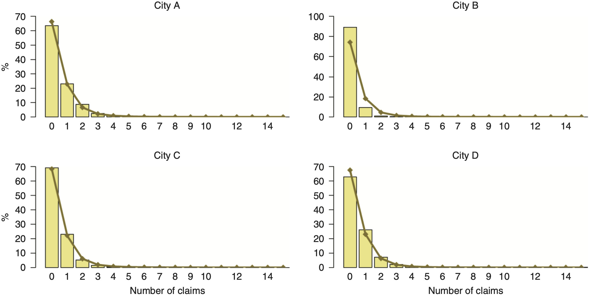
Algorithm 2 can be applied using as Zk the observed distributions of daily number of claims and claim-by-claim losses. However, to obtain forecasts using Algorithm 2, we need an approximation of the distribution of claim counts so we can adjust it to the future scenarios of claim frequencies. We considered a range of distributions to approximate the daily number of claims (Delaporte, negative binomial of types I and II, Poisson, Poisson inverse Gaussian, Sichel, and zero-inflated/adjusted Poisson) (Frees, Derrig, and Meyers 2014; Trowbridge 1989) and found that the Sichel distribution (Figure 4.1) delivers the most competitive results based on AIC. The Sichel distribution is a three-parameter compound Poisson distribution; the two-parameter form is known as the inverse Gaussian Poisson (Stein, Zucchini, and Juritz 1987). The Sichel distribution provides a flexible alternative for modeling highly skewed distributions of observed counts, and its utility in actuarial applications has been introduced by Willmot (1986), Panjer and Willmot (1990), and Willmot (1993) and then extensively studied in a variety of insurance settings (see, e.g., Bermúdez and Karlis 2012; Hera-Martines, Gil-Fana, and Vilar-Zanon 2008; Tzougas and Frangos 2014, and references therein). Table 4.1 reports the estimated parameters of the Sichel distribution fitted to the number of claims in each city in the period 2002–2011. The Kolmogorov-Smirnov and Anderson-Darling goodness of fit tests at the 5% significance level do not provide evidence against the fitted Sichel distributions for City A and City C. The null hypothesis is rejected by these tests in City B and City D due to outliers; however, the Sichel distribution still provides the best fit among all other considered distributions.
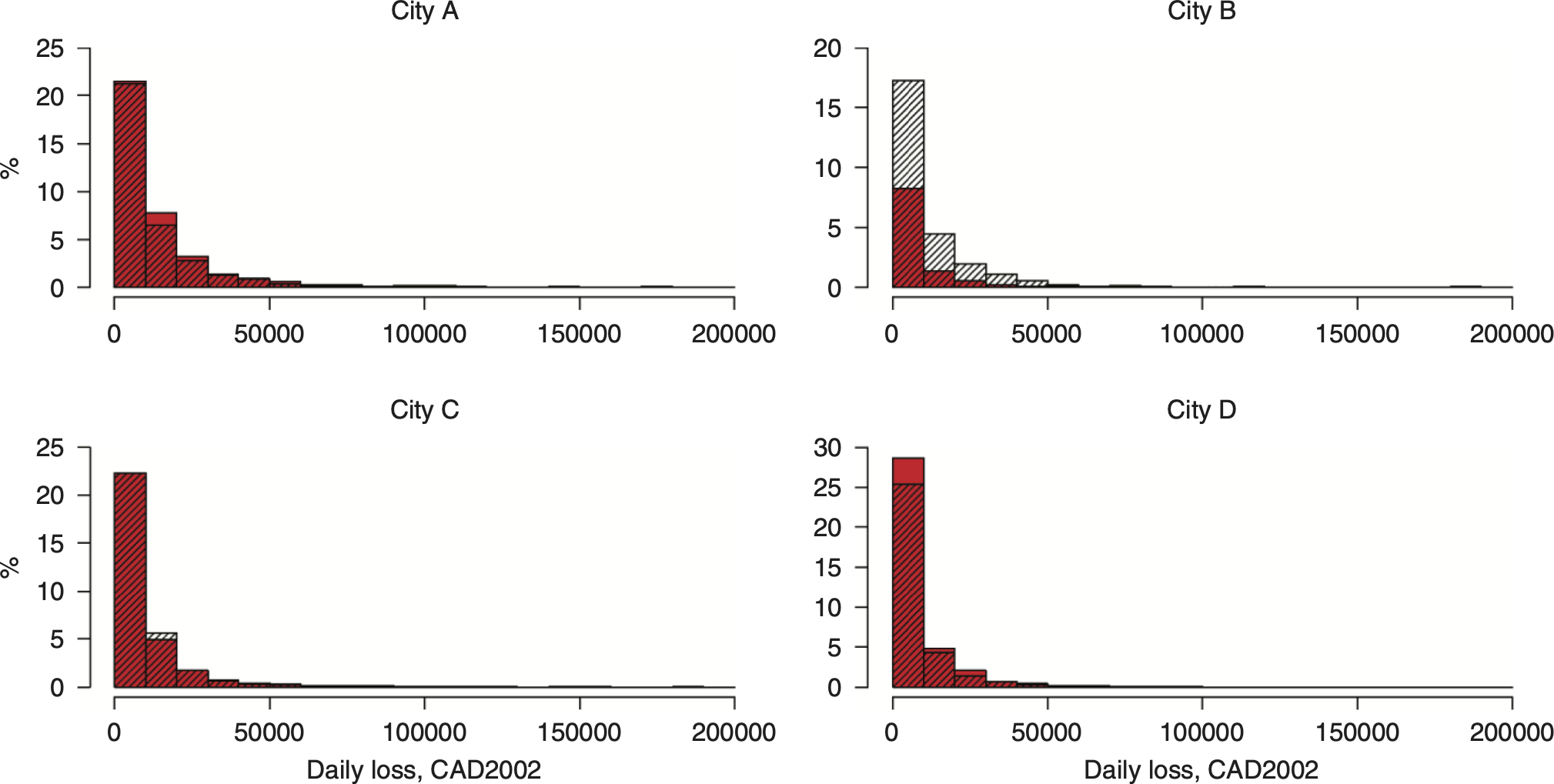
To validate the approach of approximating the number of claims with a Sichel distribution, we first consider the distributions of the observed claim severities versus their approximations using Algorithm 2 (Figure 4.2). The worst fit is observed for City B, which is not surprising given that it has very few (about 11%) days with nonzero losses, compared to more than 30% of days with losses in the other three cities. In the cases with more nonzero data (City A, City C, and City D), the simulated distributions mimic the distributions of observed severities well; therefore, we proceed with using the Sichel distribution in the CRM approach (Algorithm 2) for assessing the projected distributions of claim severities.
_and_approximated_with__algorithm_1_(271543)_(shaded)_distributions_of_dai.png)
Further, we employ results of Algorithm 1 (Section 3.2) for estimating Δ under comparison Scenario 1 (Section 3.3) for the longest period of data availability for the given scenario (10 years: 2002–2011). Table 3.2 shows the estimated increase in claim frequencies, which implies the respective changes in parameter μ of a Sichel distribution. We now apply CRM Algorithm 2, where simulations of the future number of claims in Step 1 are based on the Sichel distribution with parameters μ + Δ.
Table 4.2 presents the observed and projected percentiles for daily losses under Scenarios RCP 4.5 and RCP 8.5. All four cities exhibit noticeable increases in losses, and the most profound changes are suggested for City B (in both lower and upper percentiles). Such findings can be explained by the greater expected increase in claim frequencies (Table 3.2), the location of City B (directly on the lake), and the higher variability of fit for City B (the approximation of the number of claims by the Sichel distribution is less accurate for this city, which affects the approximation of the losses).
Remarkably, although the projected changes in mean frequency of claims in other cities are relatively synchronous (20–35% increase for City A, City C, and City D; Table 3.2), the changes in individual percentiles are more variable and range from a decline of 3% (in 75th percentile under RCP 4.5 for City A) to an increase of 94–96% (in 75th percentile for City C).
5. Conclusion
In this paper, we present a new method for modeling and forecasting house insurance losses due to noncatastrophic weather events. Our data-driven approach is based on integrating two algorithms, that is, a multivariate extension of a nonparametric method for analysis of weather-related claim counts by Soliman et al. (2015) and a simulation-based algorithm for collective risk modeling by Meyers, Klinker, and Lalonde (2003). We evaluate uncertainty due to potential differences between climate model output and weather observations and evaluate the estimated losses from two global warming scenarios. As a result, we produce a projected distribution of weather-related claim severities that intrinsically accounts for local geographical characteristics and, hence, is suitable for short- and long-term management of insurance risk due to adverse weather events. For instance, in the case of short-term risk management, when the projected precipitation is expected to exceed the critical threshold defined by our methodology, the insurance company may proactively hire more insurance assessors and loss adjusters to ensure timely processing of claims. In the case of medium- and long-term risk projections, the results of this study can be used to reevaluate insurance premiums and a range of insurance products offered in a particular area as well as to offer incentives for homeowners who reduce vulnerability of their properties to adverse weather effects and more closely collaborate with public-sector entities on introducing new weather-resistance building codes and standards.
Despite the well-documented effects of adverse weather on the insurance industry, our study is one of the first attempts to understand and evaluate the impact of noncatastrophic atmospheric events on the insurance sector, particularly home insurance (see the literature review by Lyubchich et al. 2019). Hence, we would like to conclude the paper with a discussion of a number of caveats, limitations, and open research directions.
In this proof-of-concept study, we use data from only a few locations over 10 years, but obviously, a broader spatial and temporal extent of data (to which we did not have access) would make the results more practically applicable. Climatologists traditionally use 30 years of weather data to describe expected “normal” weather; however, in a changing climate, that length of record may be too long since we expect the weather to change significantly during 30 years (Huang, van den Dool, and Barnston 1996; Livezey et al. 2007). It has been suggested that temperature and precipitation across the continental United States can be well characterized by only 10 and 15 years of data, respectively, providing the optimal predictive skill for the following year (Huang, van den Dool, and Barnston 1996). Thus, our analysis of 10 years is reasonable, though an analysis of the length of record needed for optimum predictive skill in each variable of interest could be employed by industry analysts with access to larger actuarial datasets and existing publically available weather and climate data. Expansion of this method to spatially more extensive datasets in the future would provide important information about regional patterns of expected future climate-claims relationships. With such information, we expect companies could adjust rates to more appropriately reflect the changing potential risk of “normal” weather hazards in a region.
From a practical standpoint, this type of analysis would need to be updated as model data become available (approximately every five years) to continue to use cutting-edge information about the future climate. Climate models, both regional and global, are constantly being improved. We used the latest available North American regional dynamically downscaled climate data at the time of our analysis, but the global model projection data are updated every five years for the IPCC reports, and new regional model data are available accordingly if funding for the science is continued.
The approach of our study sidesteps the traditional notion that the past is a feasible predictor of the future. In social and natural sciences, information from the past behavior of a system often is used as a predictor of the future behavior of the system. However, this assumption is valid only as long as there is a reasonable expectation that the dynamics of the system do not vary (significantly) over time. Anthropogenic climate change, however, causes a relatively rapid change in the Earth’s climate system, which puts that assumption in jeopardy for many social and environmental systems (IPCC 2014b). Milly et al. (2008) put it succinctly for the field of water management in the title of their article, “Stationarity Is Dead: Whither Water Management?” How can we assess the impact of such changes in the Earth’s climate system, and how can these changes be incorporated into insurance risk management? How are these changes distributed in space and time? This is of particular importance for regional risk management as weather-related events have long been known to induce spatial dependencies among insurance policies, often leading to undercapitalization and excessive risk taking (Cooke and Kousky 2010).
Although insurance policies are adjusted regularly and therefore can theoretically be changed to reflect current conditions, the episodic nature of many weather-related perils and relatively rapid changes cause a lag between the observed event statistics and the current real probability of an event that is increasing in frequency. How can we get ahead of this lag?
These and many other related fundamental questions about insurance risk management at the face of climate change can be addressed only if the gaps between paradigms of actuarial theory and practice, statistics, and climate sciences are bridged together, forging joint interdisciplinary efforts.
Acknowledgments
The authors thank Natalia A. Humphreys, University of Texas at Dallas; Douglas Collins, Casualty Actuarial Society (CAS); Stephen J. Ludwig, CAS; and other members of the Climate Change Committee of CAS for motivating discussions, helpful comments, and suggestions. This work was supported in part by CAS.