Recursive Credibility: Using Credibility to Blend Reserve Assumptions

undefined

1. Introduction

A recent contribution to reserving methodologies is the Munich chain ladder (MCL) of Quarg and Mack (2008), which recursively adjusts paid and reported loss development patterns based on the relative size of case reserves. It is designed to reduce the gap between paid and incurred ultimate loss indications. Performed via regression on conditional residuals, this aspect of the MCL is of seminal value to the actuarial community. Jedlicka (2007) has described multivariate extensions of the MCL that demonstrate the flexibility of regression on conditional residuals.

This paper branches off from the MCL in a different direction. It may be surprising that the MCL can be interpreted as the recursive weighting of chain ladder (CL) paid and incurred indications ($f_{s \rightarrow t}^P P_{i, s}$, $f_{s \rightarrow t}^I I_{i, s}$) with cross link^[1] (XL) paid and incurred indications ($I_{i, s} g_{s \rightarrow t}^P$, $P_{i, s} g_{s \rightarrow t}^I$), respectively. For example, a paid MCL indication, shown to the left of the approximation sign in equation (1.1) is approximately the paid CL indication weighted with the Paid XL indication to the right of the approximation sign in equation (1.1), i.e.:

$$\begin{array}{c} P_{i, s}\left(f_{s \rightarrow t}^{P}+\left(Q_{i, s}^{-1}-q_{s}^{-1}\right) \lambda^{P} \sigma_{s \rightarrow t}^{P} / \sigma_{s}^{Q^{-1}}\right) \approx \\ P_{i, s} f_{s \rightarrow t}^{P}\left(1-W_{s \rightarrow t}^{g^{P}}\right)+I_{i, s} g_{s \rightarrow t}^{P} W_{s \rightarrow t}^{g^{P}} \end{array} \tag{1.1}$$

See Appendix A for a proof of equation (1.1).

This interpretation sheds some light on a source of instability in the MCL. Basing paid development on incurred losses and incurred development on paid losses often results in zigzagging indications. If significant weight happens to be given to this zigzagging indication, it could result in some instability.

In fact, the MCL is not a strict credibility approach. The MCL formulas do not appear to have been designed to weight the CL with the XL, but rather to adjust for correlation between paid and incurred loss development using regression. Recognizing, however, that the MCL formulas come so close to the recursive application of credibility, some questions arise, such as:

1. Would recursive credibility of the CL and XL give more stable results than the MCL?

2. Can recursive credibility be applied to other loss development assumptions?

3. Can recursive credibility be applied to more than two loss development assumptions?

Recursive credibility-weighting of development assumptions can have certain unique advantages. Faced with a limited quantity of data and volatile loss development history, we often reach for multivariate tools to enhance the predictive power of our models. As a multi-assumptional tool, recursive credibility can help us to reduce the error in our model selection. Not only can it show how much weight to give each model, it can also show us when to do so. For instance, workers compensation loss development may be consistent with CL assumptions in early development ages, gradually switching over to behave more like annuity payments in later ages as indemnity and medical costs become routine and as a greater percent of remaining claimants have lifelong catastrophic injuries. Recursive credibility can give varying weight over the loss development period to different model assumptions based on these changing drivers of loss development.

Recursive credibility could also have drawbacks, such as the potential instability caused by an iterative process. One approach to mitigating this instability is utilizing the error caused by the credibility weights themselves. To understand why this is, consider the weighted sum, Z × f + (1 − Z) × g of two estimates, f and g, of the same quantity. Measurement error in this weighted sum is caused by error in all three variables, f, g and Z. Often, in determining least squares credibility, only error in f and g are considered.^[2] But error in the estimation of the variance and covariance of f and g will result in error in Z as well. Including credibility weight error in a minimization procedure results in a more stable credibility-weighted estimate than a procedure that does not recognize this source of volatility.

This paper presents a recursive credibility (RC) framework which, when using the CL and XL sub-indications (i.e., RC(f, g)^[3]), can often develop reasonable converging paid and incurred indications where the MCL fails. This RC framework borrows part of its structure from Mack’s (1994) well-known chain ladder variance estimate, which structures variance in a manner that can be mirrored by other paid and incurred model pairs, allowing recursive credibility to be used amongst these different model assumptions.

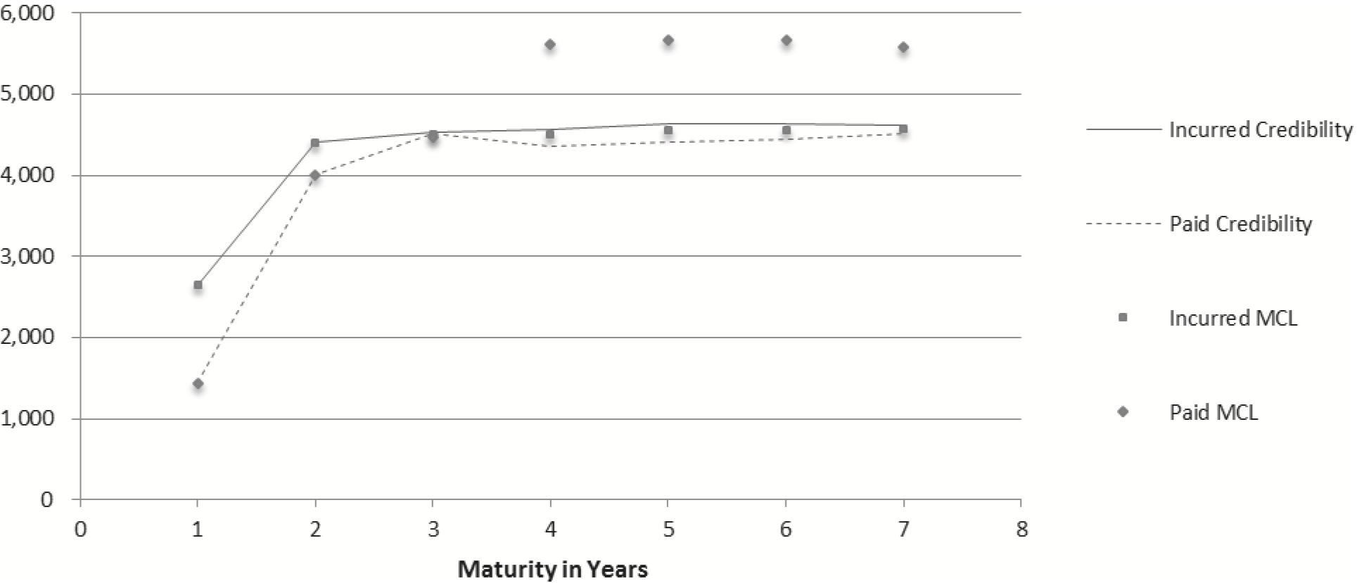
Figure 1 depicts the MCL and RC(f, g) estimates for accident year 6 using the MCL dataset (see Appendix C), where accident year 4 paid losses have been modified to be 2,286 for development years 1 through 3.

This simple modification of the data results in MCL indications that provide unrealistic loss development patterns that cross and remain divergent, with paid losses much greater than reported losses. The RC(f, g) incurred and paid indications are more stable with respect to one another, self-correcting after crossing, then converging.

A simulation documented in section 5 shows that this is not an isolated example. Rather, the MCL has occasional volatility problems, while RC(f, g) is significantly more stable, resulting in paid and incurred indications that converge quite consistently.

The credibility framework described in this paper has two distinct elements. First, it illustrates a means of recursively defining credibility. It builds a framework that borrows its structure from Thomas Mack’s (1994) chain ladder variance estimate. Second, it shows a method for determining credibility that includes credibility weight error. This method relies on a twist on credibility, thinking of it as the relative distance from a straight average. In doing so, zero-sum weights and zero-sum constants are defined. This paper combines those two elements into a single recursive credibility framework. While this paper focuses on the CL and XL assumptions, the framework has the flexibility to be used with other models as well.

Section 2 lays basic groundwork with definitions to be used throughout the paper, including model and submodel notation. Large negative credibility weights are described as motivation for measurement of credibility weight error, and error in credibility weights is shown to be equivalent to error in zero-sum weights (to be defined). Then, three key credibility assumptions are made that define a variance of zero-sum weights as an expression based on a single parameter, coined the zero-sum constant. The parameterization of the zero-sum constant is described in Appendix A.2.

In section 3, each term in Mack’s (2008) recursive variance formula^[4] for the CL is shown to be the sum of two conditional variance terms. This framework is a general variance structure that can be used with other recursive estimates. In Appendix A.3, the CL and XL are described, and similar recursive variance estimates for the XL are specified as the sum of two conditional variance terms that are analogous to the terms in Mack’s (2008) formula. Proportionality constants as well as conditional covariance terms are also defined.

Section 4 gives an estimate of the variance of a credibility-weighted indication based on two submodels in a manner that contemplates the variance of the credibility weight itself using Assumptions 1 and 2 from Section 2. Least squares regression is used to determine equations for the two weights. Appendix A.4 contains derivations of the variance and credibility equations for two sub-indications.

Section 5 demonstrates how to combine the results of Sections 3 and 4 with calculations for RC based on CL and XL sub-indications—i.e., RC(f, g). It contains results of a simulation comparing the MCL with RC(f, g). Then it ends with a comparison of the same methods using over 300 paid and reported grid pairs of industry data.

Section 6 contains concluding remarks, including commentary on strengths and weaknesses of the RC framework, and future research.

2. Loss processes, notation, and credibility weight error

This paper depends upon and builds on structures and assumptions of the MCL and Mack’s (1994) chain ladder variance equations. Thus, independence of accident year loss processes is assumed, and definitions of proportionality constants as defined in the MCL paper also apply. Where possible, MCL notational conventions have been followed. All n × n paid and incurred development triangles described herein are assumed to have no missing data. The following terminology and general assumptions will be used throughout the paper.

2.1. Paid and incurred loss processes

Let: n ∈ N be the number of accident years, and T be development time (T ⊂ N; T = {1, . . . , n}).

For i = 1, . . . , n, let $P_i=\left(P_{i, t}\right)_{t \in T}$ and $I_i=\left(I_{i, t}\right)_{t \in T}$ denote the paid and incurred processes of accident year i, given t development years respectively. The random variables P_i,t and I_i,t denote the paid and incurred losses for accident year i after t development years.

2.2. Zero-sum weights

Given credibility weights Z_i with i = 1, . . . , n, the set of W_i = Z_i − 1/n will be referred to as “zero-sum weights,” since $\sum_{i=1}^n W_i=0$. Consider a credibility-weighted sum of n indications. Letting I̅ be the mean of those indications, we can restate the credibility-weighted sum of n indications as the mean indication plus the zero-sum weighted indications, or the mean indication plus the zero-sum weighted deviations from the mean.

$$\begin{aligned} I^{R} & =\sum_{i=1}^{n} Z_{i} I^{i} \\ & =\bar{I}+\sum_{i=1}^{n}\left(W_{i}\right) I^{i} \\ & =\bar{I}+\sum_{i=1}^{n}\left(W_{i}\right)\left(I^{i}-\bar{I}\right) \end{aligned} \tag{2.1}$$

Since these zero-sum weights are simply standard credibility weights minus a constant, it is clear that they have the same variance as standard credibility weights. Therefore, determining the variance of zero-sum weights is equivalent to determining the variance of credibility weights. The second line of equation 2.1 will be used as the basis for determining the variance of the credibility-weighted sum of indications. Expressing credibility in this way will help us to manage the heteroscedasticity problem associated with credibility weight error – credibility weight error grows as distance from the average grows – while still allowing for a simple linear error minimization procedure.

2.3. Model and submodel notation

Since this paper concerns the interrelationship of models, notational conventions used in this paper are stated here for clarity. The letters f and g will refer to the CL and XL models, respectively. Loss indications, denoted P and I for paid and case incurred losses respectively, will have subscripts denoting time values and superscripts denoting the model. Development factors will be denoted by model letter, with subscripts denoting age-to-age values and superscripts denoting the loss type. For example, the paid loss chain ladder indication for accident year 3 at maturity 7 is calculated and denoted f^P_6→7P^f_3,6 = P^f_3,7.

The term “submodel” refers to a model and related assumptions that is being recursively credibility-weighted with other model assumptions to determine a final best estimate. Conversely, the term “solo model” is used to distinguish a model that is implemented as a stand-alone model.

An RC indication will be notated with a capital R superscript. Thus the RC paid loss indication for accident year 3 at maturity 7 is denoted P^R_3,7. This means that one or more submodels have been credibility-weighted to give this indication. An RC indication could conceivably refer to a single model credibility indication, in which the single model would always receive full credibility. Thus, RC notation is a generalization of independent model notation.

Functions, such as variance or correlation, will be named followed by parentheses. A hat (^) symbol specifies an estimate rather than an actual or theoretical value. For instance, Vâr(P^f_3,7) = σ̂²(P^f_3,7) is the estimate of the variance of the CL paid loss indication for accident year 3, at maturity 7.

Proportionality constants will be denoted with a sigma, with superscripts denoting both the model and the loss type and subscripts denoting the age-to-age values. For instance, $\hat{\sigma}_{6 \rightarrow 7}^{f P}$ is the paid CL proportionality constant for development from age 6 to 7. Zero-sum constants will be denoted similarly, except with a subscripted W. For example, $\hat{\sigma}_W^{f P}$ denotes the zero-sum constant for the paid CL.

2.4. Negative credibility weights

Least squares credibility that contemplates covariance of indications can result in negative credibility weights. A question that may arise is “What do negative credibility weights mean?” As an illustration, assume that indication A always deviates from Actual by twice the deviation of indication B. Then

A − Actual = 2(B − Actual). Thus, Actual = 2B + (−1) A. In this instance, Actual can be determined using solution credibility weights −1 and 2. In general, for two indications A and B, when the quantities (A − Actual) and (B − Actual) are highly correlated, negative credibility weights can result.

As a second illustration, assume that A historically deviates from Actual by .99 times the deviation of B. Then A − Actual = .99(B − Actual), and Actual = 100A − 99B. Clearly, the parameter error contribution to total estimation error associated with credibility weights of 100 and −99 could be significant.

This parameter error could cause significant distortions to least squares credibility-weighted indications. Recognizing error in the credibility weights can help to mitigate these distortions without adding prohibitively to the complexity of a credibility framework.

2.5. Zero-sum weight error

In addition to assumptions regarding loss development, variance and independence, RC depends on the following key assumptions concerning zero-sum weight error.

Assumption 1: Given an RC indication based on two sub-indications, parameter variance of the zero-sum weights is inversely proportional to the squared difference between the sub-indications.

Appendix A.2 shows that this assumption is based on actual process error patterns.

Assumption 2: Given an RC indication based on two sub-indications, parameter variance of the zero-sum weights is proportional with $\hat{W}^{f^2} \operatorname{Var}\left(I^f-I^g\right)$.

This assumption forces the error in the credibility weight to equal zero when the weights are equivalent (when zero-sum weights equal zero). The error then increases as the magnitude of the zero-sum weight increases. This assumption also recognizes that error in the weight is proportional to error in the underlying sub-indications. Appendix A.2 gives a more detailed explanation of this assumption.

Assumptions 1 and 2 Combined: The parameter variance of a two-indication zero-sum weight is proportional with a scaling expression.

Given the weighted average of two sub-indications {I^f, I^g}, based on assumptions 1 and 2, there exists a zero-sum constant σ^I_W, such that:

$$\operatorname{Var}\left(W^{f}\right)=\sigma_{w}^{I^{2}} \frac{W^{f 2} \operatorname{Var}\left(I^{f}-I^{g}\right)}{\left(I^{f}-I^{g}\right)^{2}} \tag{2.2}$$

Based on this assumption, the variance of the zero-sum weights (and thus the credibility weights) increases with the magnitude of the zero-sum weights themselves. This mitigates the possibility of massive credibility weights being output in an error minimization procedure.

Assumption 3: Two-indication zero-sum weights are independent of sub-indication differences and sub-indication sums as well as the ratios of the sub-indication difference over the sub-indication sum.

This assumption is made to simplify the derivation of the variance of a credibility-weighted sum of indications. It makes zero-sum weights behave as constants in sub-indication covariance expressions. Although this is not a perfect assumption, it is reasonable because:

1. The absolute magnitude of indications should clearly be independent of the credibility weights.

2. The impact of the scaled sub-indication difference on the credibility weights will be largely mitigated by accounting for variance of the credibility weights in the total variance. The large weights that might have been caused by small ratios should not occur.

3. Submodel recursive variance and covariance expressions

To define least-squares credibility of loss indications recursively, the variance of those indications must also be defined recursively. To see how to accomplish this, consider the following two examples.

First, if I₁ is actual incurred losses at time 1 and a function applied to incurred losses at time 1 is $f_{1 \rightarrow 2}^I$, then the resulting indication, $\hat{I}_2=\hat{f}_{1 \rightarrow 2}^I\left(I_1\right)$. The second function $f_{2 \rightarrow 3}^I$ is then applied not to actual data, but to the prior indication. That is $\hat{I}_3$ = $\hat{f}_{2 \rightarrow 3}^I\left(\hat{I}_2\right)$ = $\hat{f}_{2 \rightarrow 3}^I\left(\hat{f}_{1 \rightarrow 2}^I\left(I_1\right)\right)$.

As a second example, if I₂ is actual incurred losses at time two, then $\hat{I}_3=\hat{f}_{2 \rightarrow 3}^I\left(I_2\right)$.

Even if Î₂ from the first example equals I₂ from the second example, the variance of Î₃ from the first should not equal the variance of Î₃ from the second. The variance of a function performed on a known amount should be different than the variance of the same function performed on an estimate. The variance of Î₃ from the first example must contemplate the error due to $\hat{f}_{2 \rightarrow 3}^I$ as well as the error due to Î₂. The variance of Î₃ from the second example only needs to contemplate the error due to $\hat{f}_{2 \rightarrow 3}^I$.

This suggests that the variance of a recursive estimate can be considered in two parts, the variance due to error in the function given the prior indication and the variance due to error in the prior indication given the function. Thomas Mack (2008) has presented his well-known chain ladder variance equations recursively, yielding a variance estimate for each recursive loss indication. Thus, the chain ladder (f) model can be used as one element in an RC relationship.

The conditional structure of Mack’s (2008) CL variance formula can also serve as a general framework for the variance of some other indications, and this framework facilitates RC relationships. More specifically, each recursive element of Mack’s CL variance formula is the sum of two conditional variance terms, where the two conditions are the known prior losses (KPL) condition and the known development factors (KDF) condition. The KPL and KDF conditions will be used throughout the paper for different models, with the same meaning as defined below.

For this framework to remain simple, it will be assumed that volatility given KPL and volatility given KDF are independent of one another across indications, and this will allow the sum of the covariance given KPL and the covariance given KDF to equal the total covariance.

3.1. The known prior losses (KPL) condition

Being given the set, $B_i(s)=\left\{P_{i, 1}, \ldots, P_{i, s} ; I_{i, 1}, \ldots, I_{i,s}\right\}$, of paid and incurred development for accident year i until the end of development year s, implies that loss development through development year s is known and constant. This condition is key to Mack’s recursive variance calculation, since it allows the variance to be separated into the variance given KPL through age s (expressed as the total expression in equation (3.1)) and the remaining variance, stated next.

$$\operatorname{Var}\left(I_{i, t}^{f} \mid B_{i}(s)\right)=I_{i, s}^{R^{2}}\left(\frac{\sigma_{s \rightarrow t}^{f l}{\mathstrut}^{2}}{I_{i, s}^{R}}+\frac{\sigma_{s \rightarrow t}^{f f 2}}{\sum_{j=1}^{n-s} I_{j, s}}\right) \tag{3.1}$$

Recalling that RC notation is a generalization of independent model notation, where R is allowed to equal f, equation (3.1) is a summand from Mack’s recursive variance formula for incurred losses.

3.2. The known development factors (KDF) condition

The variance that remains, excluding the KPL variance is the KDF variance, described here. Suppose we have three pairs of loss development assumptions f, g, and h. Being given the set $D_{s \rightarrow t}=\left\{f_{s \rightarrow t}^I, f_{s \rightarrow t}^P ; g_{s \rightarrow t}^I\right.$, $\left.g_{s \rightarrow t}^P ; h_{s \rightarrow t}^I, h_{s \rightarrow t}^P\right\}$ of factors based on these assumptions, where s, t ∈ T and t = s + 1 implies that the factors that develop losses from time s to time t are known and constant. Equation (3.2) expresses this variance given KDF, i.e., the variance of the prior indication times the squared development factor:

$$\operatorname{Var}\left(I_{i, t}^{f} \mid D_{s \rightarrow t}\right)=\operatorname{Var}\left(I_{i, s}^{R}\right) f_{s \rightarrow t}^{I}{\mathstrut}^{2} \tag{3.2}$$

Reducing the set $D_{s \rightarrow t}=\left\{f_{s \rightarrow t}^I, f_{s \rightarrow t}^P\right\}$ and changing R to f would make equation (3.2) the second summand from Mack’s recursive variance calculation for incurred losses.

3.3. Mack’s recursive chain ladder variance term

For incurred and paid losses, the recursive version of Mack’s chain ladder variance expression is thus the sum of the variance given known development factors from development year s to t and the variance given known losses through development year s.

$$\begin{aligned} \operatorname{Var}\left(I_{i, t}^{f}\right) & =\operatorname{Var}\left(I_{i, t}^{f} \mid D_{s \rightarrow t}\right)+\operatorname{Var}\left(I_{i, t}^{f} \mid B_{i}(s)\right) \\ & =\operatorname{Var}\left(I_{i, s}^{R}\right) f_{s \rightarrow t}^{I}+I_{i, s}^{R^{2}}\left(\frac{\sigma_{s \rightarrow t}^{f I}{\mathstrut}^{2}}{I_{i, s}^{R}}+\frac{\sigma_{s \rightarrow t}^{f-2}}{\sum_{j=1}^{n-s} I_{j, s}}\right) \end{aligned} \tag{3.3}$$

$$\begin{aligned} \operatorname{Var}\left(P_{i, t}^{f}\right) & =\operatorname{Var}\left(P_{i, t}^{f} \mid D_{s \rightarrow t}\right)+\operatorname{Var}\left(P_{i, t}^{f} \mid B_{i}(s)\right) \\ & =\operatorname{Var}\left(P_{i, s}^{R}\right) f_{s \rightarrow t}^{P 2}+P_{i, s}^{R^{2}}\left(\frac{\sigma_{s \rightarrow t}^{f P 2}}{P_{i, s}^{R}}+\frac{\sigma_{s \rightarrow t}^{f P}}{\sum_{j=1}^{n-s} P_{j, s}}\right) \end{aligned} \tag{3.4}$$

Converting from the submodel recursive variance formulas of equations 3.3 and 3.4 to solo model formulas by allowing R to equal f would precisely make these equations Mack’s recursive variance formulas for incurred and paid losses for a single accident year (2008).

In Appendix A.3, CL and XL submodel indications are defined, and recursive variance equations are described as the sum of variance given KPL and variance given KDF. Additionally, proportionality constants are defined, as well as KPL correlation and KDF covariance for the given submodels.

4. Credibility procedure: Contemplating error in the weights

By considering the variance of the credibility-weighted sum of two indications (equation (2.1)) and contemplating error in the credibility weights (equation (2.2)) the variance of the credibility-weighted estimate can be determined (equation (4.1)). The derivation of this estimate, which depends on Assumption 3 that credibility weights are constant in the covariance terms, and W^fI_i,t selected to minimize the variance, is shown in Appendix A.4.

$$\begin{aligned} \operatorname{Var}\left(Z_{i, t}^{f} I_{i, t}^{f}+Z_{i, t}^{g l} I_{i, t}^{g}\right)= & 0.25 \operatorname{Var}\left(I_{i, t}^{f}+I_{i, t}^{g}\right) \\ & -0.5\left(\operatorname{Var}\left(I_{i, t}^{g}\right)-\operatorname{Var}\left(I_{i, t}^{f}\right)\right) W_{i, t}^{f f} \end{aligned} \tag{4.1}$$

Equation (4.2) is the theoretical zero-sum weight as derived in Appendix A.4.

$$W_{i, t}^{f t}=\frac{0.5\left(\operatorname{Var}\left(I_{i, t}^{g}\right)-\operatorname{Var}\left(I_{i, t}^{f}\right)\right)\left(I_{i, t}^{f}-I_{i, t}^{g}\right)^{2}}{\operatorname{Var}\left(I_{i, t}^{f}-I_{i, t}^{g}\right)\binom{\left(I_{i, t}^{f}-I_{i, t}^{g}\right)^{2}+\sigma_{W}^{I}\left(I_{i, t}^{f}-I_{i, t}^{g}\right)^{2}}{+\sigma_{W}^{I}{\mathstrut}^{2} \operatorname{Var}\left(I_{i, t}^{f}-I_{i, t}^{g}\right)}} \tag{4.2}$$

Following are descriptions of a few final details needed to complete a recursive credibility indication.

First, in addition to individual loss indications, variance terms, and a zero-sum parameter, equations (4.1) and (4.2) contain the expressions Var(I^f_i,t − I^g_i,t) and Var(I^f_i,t + I^g_i,t), which can be expanded to Var(I^f_i,t) + Var(I^g_i,t) − 2Cov(I^f_i,t, I^g_i,t) and Var(I^f_i,t) + Var(I^g_i,t) + 2Cov(I^f_i,t, I^g_i,t) respectively.

Next, by the assumption from Section 3 that volatility given KPL and volatility given KDF are independent of one another across sub-indications, the covariance term can be expressed as follows:

$$\operatorname{Cov}\left(I_{i, t}^{f}, I_{i, t}^{g}\right)=\operatorname{Cov}\left(I_{i, t}^{f}, I_{i, t}^{g} \mid D_{s \rightarrow t}\right)+\operatorname{Cov}\left(I_{i, t}^{f}, I_{i, t}^{g} \mid B_{i}(s)\right) \tag{4.3}$$

Both sets of conditional covariance terms can be fully expressed using equations (A.23) to (A.27).

We now have all the necessary elements to square a triangle with a recursive credibility indication. Below, the steps are listed sequentially and they are demonstrated with a numerical example in the next section.

Parameter Steps: We use the data in the upper triangular matrix to calculate parameters needed for the sub-indication models and for implementing recursive credibility.

1. Step P1: We calculate submodel parameters and values associated with the upper triangular matrix.

   1. Step P1a: Development factors (based on volume-weighted averages)

   2. Step P1b: Indications (using equations (A.14), (A.15), (A.18), and (A.19))

   3. Step P1c: Proportionality constants (using equation (A.22))

   4. Step P1d: Variances (using equations (A.16), (A.17), (A.20), and (A.21))

2. Step P2: We calculate RC parameters associated with the upper triangular matrix.

   1. Step P2a: Correlations given known prior losses (using equations (A.23) and (A.24)).

   2. Step P2b: Zero-sum constants σ^I_W and σ^P_W (using equation (A.12)).

Development Steps: We use the values calculated from the upper triangular matrix in Steps P1 and P2 to iteratively add diagonals to the development triangle, “squaring” the triangle.

1. Step D1: Using parameters from Step P1, we calculate the incurred and paid sub-indications I^f_i,t, I^g_i,t, P^f_i,t and P^g_i,t, and the submodel variance terms.

2. Step D2: Relying on equation (4.3), we use KPL correlations from step P2 and KDF covariance terms from equations (A.25) and (A.26) to determine the total covariance of the underlying sub-indications.

3. Step D3: Using equation (4.2) and zero-sum constants from Step P2, we calculate the zero-sum weights W^fI_i,t and W^gI_i,t (and likewise W^fP_i,t and W^gP_i,t).

4. Step D4: Using the zero-sum weights calculated in Step D3 and equation (2.1), we calculate the RC indication I^R_i,t (and likewise P^R_i,t).

   $$I_{i, t}^{R}=0.5\left(I_{i, t}^{f}+I_{i, t}^{g}\right)+I_{i, t}^{f} W_{i, t}^{f I}+I_{i, t}^{g} W_{i, t}^{g I} \tag{4.4}$$

   $$P_{i, t}^{R}=0.5\left(P_{i, t}^{f}+P_{i, t}^{g}\right)+P_{i, t}^{f} W_{i, t}^{f P}+P_{i, t}^{s} W_{i, t}^{g P} \tag{4.5}$$

5. Step D5: Using equation (4.1) and the weights calculated in Step D3, we calculate the variance of the RC indication at time t, Var(I^R_i,t) (and likewise Var(P^R_i,t)).

5. Numerical example

To demonstrate recursive credibility with a numerical example, we will first calculate parameters and then two years of development for the fifth accident year of the MCL dataset (tables B.1 and B.2). We will follow the (P)arameter and (D)evelopment steps outlined above. Then we will compare RC(f, g) paid and incurred loss development patterns to those implied by the CL and XL models.

At the end of this section, some statistics are documented from a simulation directly comparing the MCL with RC(f, g). These statistics demonstrate that the RC(f, g) indications are more stable than the MCL derived indications.

5.1. Parameter steps

• Step P1: We calculate submodel parameters and indications based on the upper triangular matrix

  • Step P1a: Development factors (based on volume-weighted averages)

Table 1 contains all-year weighted average development factors, calculated using historical data from tables B.1 and B.2. As an example, the 3-4 factor for the Paid XL and the 4-5 factor for the Paid CL are calculated as follows:

$$\hat{g}_{3 \rightarrow 4}^{P}=\frac{\sum_{i} P_{i, 4}}{\sum_{i} I_{i, 3}}=\frac{2024+2232+4416+5850}{2134+2466+4698+6070}=0.945$$

$$\hat{f}_{4 \rightarrow 5}^{p}=\frac{\sum_{i} P_{i, 5}}{\sum_{i} P_{i, 4}}=\frac{2074+2284+4494}{2024+2232+4416}=1.021$$

• Step P1b: Indications (using equations (A.14), (A.15), (A.18), and (A.19))

Tables C.1, C.2, C.3, and C.4 contain upper triangular matrix indications, calculated by multiplying losses from Tables B.1 and B.2 by development factors from Table 1. Each indication in the upper triangular matrix is calculated as the actual loss times the development factor. For example:

$$\hat{P}_{5,3}^{s}=\hat{g}_{2 \rightarrow 3}^{p} I_{5,2}=.945 \times 4882=4613$$

• Step P1c: Proportionality constants (using equation (A.22))

Based on equation (A.22), the proportionality constant for each submodel by loss development maturity is the square root of the sum of the squared, scaled loss indication residuals divided by their degrees of freedom (where the residuals are scaled by prior historical losses). As an example, we use the indications from Table C.4 and the losses from Table B.1 to illustrate the incurred XL proportionality constant from age 3 to 4.

$$\begin{aligned} \hat{\sigma}_{3 \rightarrow 4}^{g l} & =\sqrt{\frac{\sum_{i=1}^{4}\left(I_{i, 4}-\hat{I}_{i, 4}^{s}\right)^{2} / I_{i, 3}}{7-3-1}} \\ & =\sqrt{\left[\begin{array}{l} \left.\frac{(2144-2146)^{2}}{2134}+\frac{(2480-2355)^{2}}{2466}\right] \\ \left.+\frac{(4600-4631)^{2}}{4698}+\frac{(6142-6234)^{2}}{6070}\right] \end{array}\right.}=1.63 \end{aligned}$$

The paid and incurred CL and XL proportionality constants by age are listed in Table 2.

• Step P1d: Variances (using equations (A.16), (A.17), (A.20), and (A.21))

Variances for the upper triangular matrix of indications are calculated using data from Tables B.1 and B.2, and proportionality constants from Table 2. Since each entry in the upper triangular matrix of indications is calculated using only historical losses multiplied by a single factor, the KDF variance terms are always equal to zero, which simplifies all the upper triangular matrix variance terms to be only KPL variance terms. For example:

$$\begin{aligned} \operatorname{Vâr}\left(P_{3,5}^{g}\right) & =P_{3,4}{\mathstrut}^{2}\left(\frac{\hat{\boldsymbol{\sigma}}_{4 \rightarrow 5}^{g^{P}}{\mathstrut}^{2}}{P_{3,4}}+\frac{\hat{\boldsymbol{\sigma}}_{4 \rightarrow 5}^{g^{P}}{\mathstrut}^{2}}{\sum_{j=1}^{3} P_{j, 4}}\right) \\ & =4416^{2}\left(\frac{1.69^{2}}{4416}+\frac{1.69^{2}}{2024+2232+4416}\right) \\ & =18972 \end{aligned}$$

The upper triangular matrix variances are presented in Tables C.5, C.6, C.7, and C.8.

• Step P2: We calculate RC parameters associated with the upper triangular matrix.

In Step P1, we calculated values associated with each of the individual submodels. In Step P2, we calculate parameters necessary to combine the information from the submodels.

• Step P2a: Correlation given known prior losses (using equations (A.23) and (A.24)).

The correlation between loss indications given KPL is calculated across the upper triangular matrix (using equation (A.24)) as the sum of the product of conditional residual pairs divided by the degrees of freedom. Thus, to calculate the correlation given KPL, we first need conditional residuals.

A conditional residual (defined by equation (A.23)) is a scaled residual divided by the proportionality constant (where the scaling term is the square root of the prior age losses). Thus, a paid XL conditional residual for accident year 2 at age 4 is $\frac{(2232-2330)}{\sqrt{2162}} / 1.52=-1.39 .$Based on the conditional residuals shown below in Tables 3 and 4, we can now calculate the correlation given KPL as

$$\begin{aligned} \hat{\rho}\left(P^{f}, P^{z} \mid K P L\right) & =\frac{\left[\begin{array}{l} (1.27)(1.24)+(-0.14)(-0.45) \\ +\cdots+(.18)(1.66)+(.57)(.97) \end{array}\right]}{(6)(5) / 2} \\ & =-0.0765 \end{aligned}$$

An incurred CL conditional residual for accident year 5 at age 3 is $\frac{(4852-4973)}{\sqrt{4882}} / 2.54=-0.68$Based on the conditional residuals shown below in Tables 5 and 6, we can calculate the correlation given KPL as ρ̂(I^f, I^g | KPL) = 0.0355.

• Step P2b: Zero-sum constants (using equation (A.12))

Zero-sum constants can be thought of as a portion of the standardized deviation of zero-sum weights from actual weights that would produce a correct solution (zero-sum residuals). To calculate a single paid zero-sum residual, take the difference between a solution weight W^fP_i,t such that $\left(W_{i, t}^{f P}-0.5\right) \hat{P}_{i, t}^f+\left(W_{i, t}^{f P}+0.5\right)$ $\hat{P}_{i, t}^g=P_{i, t}$, calculated $W_{i, t}^{f P}=\frac{P_{i, t}-\hat{P}_{i, t}^{g}}{\hat{P}_{i, t}^{f}-\hat{P}_{i, t}^{g}}-0.5$ and an estimated weight, based on equation (4.2), and setting the zero-sum constant equal to zero, calculated $\hat{W}_{i, t}^{f p}=\frac{0.5\left(\operatorname{Varr}\left(P_{i, t}^{s}\right)-\operatorname{Vâr}\left(P_{i, t}^{f}\right)\right)}{\operatorname{Vâr}\left(P_{i, t}^{f}-P_{i, t}^{s}\right)} .$ Using paid indications from Tables C.1 and C.2, paid variances from Tables C.5 and C.6 and the KPL correlation calculated in Step P2a, the zero-sum weight residual for accident year 5, at time 2 is calculated.

$$\begin{array}{l} W_{5,2}^{f p}-\hat{W}_{5,2}^{f p}=\left(\frac{P_{5,2}-\hat{P}_{5,2}^{g}}{\hat{P}_{5,2}^{f}-\hat{P}_{5,2}^{s}}-0.5\right)-\left(\frac{0.5\binom{\operatorname{Vâr}\left(P_{5,2}^{s}\right)}{-\operatorname{Vâr}\left(P_{5,2}^{f}\right)}}{\operatorname{Vâr}\left(P_{5,2}^{f}-P_{5,2}^{s}\right)}\right) \\ \\ =\left(\frac{3778-3944}{4552-3944}-0.5\right)-\left(\frac{0.5(459556-412993)}{\left[\begin{array}{c} 412993+459556 \\ -2(-.0765) \times \\ \sqrt{412993 \times 459556} \end{array}\right]}\right) \\ \quad=(-0.77)-(0.02) \\ \quad=-0.80 \end{array}$$

To scale the paid zero-sum residual, the scaling factor for accident year 5 at time 2 is

$$\begin{array}{l} \sqrt{\frac{\operatorname{Vâr}\left(Z_{5,2}^{f P} P_{5,2}^{f}+Z_{5,2}^{g P} P_{5,2}^{g}\right)}{\left(\hat{P}_{5,2}^{f}-\hat{P}_{5,2}^{g}\right)^{2}}} \\ =\sqrt{\frac{\left[\begin{array}{c} (0.52)^{2} 412993+(0.48)^{2} 459556+ \\ 2(-.0765)(0.52)(0.48)) \sqrt{(412993)(459556)}] \end{array}\right.}{(4552-3944)^{2}}} \\ =0.7370 \end{array}$$

Thus, the scaled residual is −0.80 / 0.7370 = −1.08. Table 7 contains for the upper triangular matrix, the set of scaled residuals for the paid CL (which are the negative scaled residuals for the Paid XL).

Based on these paid scaled zero-sum residuals, the paid zero-sum constant is calculated based on equation (A.12) as follows:

$$\begin{aligned} \hat{\sigma}_{w}^{P} & =\sqrt{\left.\sum_{i=1}^{n-1} \sum_{t=2}^{n+1-i} \frac{\left(\frac{\left(W_{i t}^{f P}-\hat{W}_{i, t}^{f p}\right)^{2}\left(\hat{P}_{i, t}^{f}-\hat{P}_{i, t}^{s}\right)^{2}}{\left(\frac{(n-1)(n-2)}{2}\right)\left(\frac{\left.\hat{W}_{i t}\right)}{f 2}\right) \hat{\sigma}\left(P_{i, t}^{f} \hat{\sigma}\left(P_{i, t}^{s}\right)\right.}\right)}{2}\right)} \\ & =\sqrt{\frac{1.79^{2}+(-0.40)^{2}+\cdots+(-1.15)^{2}+(-1.05)^{2}}{(6 \times 5 / 2)(8 \times 5 / 2)}} \\ & =0.2167 \end{aligned}$$

The incurred zero-sum constant can be likewise calculated to be σ̂^I_W = 0.2015. The purpose of these parameters is to serve as a measure of the uncertainty in the credibility weights due to the magnitude of the weight itself, which will help to mitigate error due to unreasonably large weights.

We have completed the initial parameter steps of the RC framework. Steps 3 through 9 are recursive development steps, which we will calculate for accident year 5.

5.2. Development steps

• Step D1 (1st new diagonal): We calculate submodel indications and submodel variance terms

For the first new diagonal, we use historical losses from Tables B.1 and B.2 and development factors from Table 1.

$$\begin{array}{l} \hat{P}_{5,4}^{s}=\hat{g}_{3 \rightarrow 4}^{P} I_{5,3}=.945 \times 4852=4585, \\ \hat{P}_{5,4}^{f}=\hat{f}_{3 \rightarrow 4}^{P} P_{5,3}=1.029 \times 4648=4784 \end{array}$$

$$\begin{array}{l} \hat{I}_{5,4}^{g}=\hat{g}_{3 \rightarrow 4}^{I} P_{5,3}=1.089 \times 4648=5062, \\ \hat{I}_{5,4}^{f}=\hat{f}_{3 \rightarrow 4}^{I} I_{5,3}=1.000 \times 4852=4851 \end{array}$$

These submodels can be found on Tables C.1, C.2, C.3, and C.4.

To calculate the submodel variance terms for the first new diagonal, since the prior diagonal is actual historical losses, equations (A.16), (A.17), (A.20) and (A.21) can be simplified. The variance given KDF is equal to zero, and we use historical losses from Tables B.1 and B.2 and proportionality constants from Table 2.

$$\begin{array}{l} \operatorname{Var}\left(P_{5,4}^{g}\right)=P_{5,3}^{2}\left(\frac{\hat{\sigma}_{3 \rightarrow 4}^{g^{2}}}{P_{5,3}^{2}}+\frac{\hat{\sigma}_{3 \rightarrow 4}^{g P^{2}}}{\sum_{j=1}^{4} P_{j, 3}}\right) \\ \quad=4648^{2}\left(\frac{1.52^{2}}{4648}+\frac{1.52^{2}}{1970+2162+4252+5724}\right) \\ \quad=14208 \end{array}$$

$$\begin{array}{l} \operatorname{Varr}\left(P_{5,4}^{f}\right)=P_{5,3}{\mathstrut}^{2}\left(\frac{\hat{\boldsymbol{\sigma}}_{3 \rightarrow 4}^{f P^{2}}}{P_{5,3}}+\frac{\left.{\hat{\hat{\sigma}_{3 \rightarrow 4}}{\mathstrut}^{f P^{2}}}^{\sum_{j=1}^{3} P_{j, 3}}\right)}{2}\right) \\ =4648^{2}\left(\frac{0.48^{2}}{4648}+\frac{0.48^{2}}{1970+2162+4252+5724}\right) \\ =1435 \end{array}$$

$$\begin{array}{l} \operatorname{Var}\left(I_{5,4}^{g}\right)=I_{5,3}{\mathstrut}^{2}\left(\frac{\hat{\sigma}_{3 \rightarrow 4}^{g I}{\mathstrut}^{2}}{I_{5,3}}+\frac{\hat{\sigma}_{3 \rightarrow 4}^{g l{\mathstrut}^{2}}}{\sum_{j=1}^{4} I_{j, 3}}\right) \\ \quad=4852^{2}\left(\frac{1.63^{2}}{4852}+\frac{1.63^{2}}{2134+2466+4698+6070}\right) \\ \quad=16965 \end{array}$$

$$\begin{array}{l} \operatorname{Vâr}\left(I_{5,4}^{f}\right)=I_{5,3}{\mathstrut}^{2}\left(\frac{\hat{\sigma}_{3 \rightarrow 4}^{f r}{\mathstrut}^{2}}{I_{5,3}}+\frac{\hat{\sigma}_{3 \rightarrow 4}^{f{\mathstrut}^{2}}}{\sum_{j=1}^{3} I_{j, 3}}\right) \\ \quad=4852^{2}\left(\frac{1.00^{2}}{4852}+\frac{1.00^{2}}{2134+2466+4698+6070}\right) \\ \quad=6436 \end{array}$$

These submodel variances can be found on Tables C.5, C.6, C.7, and C.8.

• Step D2 (1st new diagonal): We calculate the total covariance of the underlying indications

For the first new diagonal, since variance given KDF is equal to zero, the total covariance is equal to covariance given KPL. The correlation given KPL was calculated in step P2, and the submodel variance terms were calculated in step D1.

$$\begin{array}{l} \operatorname{Cov}\left(P_{5,4}^{g}, P_{5,4}^{f}\right) \\ \quad=\hat{\rho}\left(P^{f}, P^{g} \mid K P L\right) \hat{\sigma}\left(P_{5,4}^{g} \mid B_{5}(3)\right) \hat{\sigma}\left(P_{5,4}^{f} \mid B_{5}(3)\right) \\ \quad=-0.0765 \sqrt{14208} \sqrt{1435}=-346 \end{array}$$

$$\begin{array}{l} \operatorname{Cov}\left(I_{5,4}^{g}, I_{5,4}^{f}\right) \\ \quad=\hat{\rho}\left(I^{f}, I^{g} \mid K P L\right) \hat{\sigma}\left(I_{5,4}^{g} \mid B_{5}(3)\right) \hat{\sigma}\left(I_{5,4}^{f} \mid B_{5}(3)\right) \\ \quad=0.0355 \sqrt{16965} \sqrt{6436}=371 \end{array}$$

• Step D3 (1st new diagonal): We calculate the zero-sum weights

Using equation (4.2), we calculate the zero-sum weights Ŵ^fI_i,t and Ŵ^gI_i,t (and likewise Ŵ^fP_i,t and Ŵ^gP_i,t). We utilize the zero-sum constants from Step P2b, the submodel indications and submodel variance terms from Step D1 and the covariance terms from Step D2. For paid indications, the zero-sum weight is calculated as follows:

$$\begin{array}{l} \hat{W}_{5,4}^{f p}=\frac{0.5\left(\operatorname{Vâr}\left(P_{5,4}^{g}\right)-\operatorname{Vâr}\left(P_{5,4}^{f}\right)\right)\left(\hat{P}_{5,4}^{f}-\hat{P}_{5,4}^{g}\right)^{2}}{\operatorname{Vâr}\left(P_{5,4}^{f}-P_{5,4}^{g}\right)\binom{\left.\left(\hat{P}_{5,4}^{f}-\hat{P}_{5,4}^{g}\right)^{2}+\hat{\sigma}_{w}^{p}\left(\hat{P}_{5,4}^{f}-\hat{P}_{5,4}^{g}\right)^{2}\right)}{+\hat{\sigma}_{w}^{p} \operatorname{Vâr}\left(P_{5,4}^{f}-P_{5,4}^{g}\right)}} \\ =\frac{0.5(14208-1435)(4784-4585)^{2}}{\left\{\begin{array}{c} (1435+14208-2(-.0765) \sqrt{1435} \sqrt{14208}) \\ \left.\times\left[\begin{array}{c} (4784-4585)^{2}+.2167^{2}(4784-4585)^{2} \\ +.2167^{2}\binom{1435+14208-2(-.0765)}{\sqrt{1435} \sqrt{14208}} \end{array}\right]\right\} \end{array}\right\},} \\ =0.367=-\hat{W}_{5,4}^{g P} \end{array}$$

For incurred indications, the zero-sum weight is calculated as follows:

$$\begin{array}{l} \hat{W}_{5,4}^{f l}=\frac{0.5\left(\operatorname{Varr}\left(I_{5,4}^{g}\right)-\operatorname{Varr}\left(I_{5,4}^{f}\right)\right)\left(\hat{I}_{5,4}^{f}-\hat{I}_{5,4}^{g}\right)^{2}}{\operatorname{Varr}\left(I_{5,4}^{f}-I_{5,4}^{g}\right)\left(\begin{array}{c} \left(\hat{I}_{5,4}^{f}-\hat{I}_{5,4}^{g}\right)^{2}+\hat{\sigma}_{w}^{I}\left(\hat{I}_{5,4}^{f}-\hat{I}_{5,4}^{g}\right)^{2} \\ +\hat{\sigma}_{w}^{I} 2 \\ \operatorname{Var}\left(I_{5,4}^{f}-I_{5,4}^{g}\right) \end{array}\right)} \\ =\frac{0.5(6436-16965)(4851-5062)^{2}}{\left\{\begin{array}{c} (16965+6436-2(.0355) \sqrt{16965} \sqrt{6436}) \\ \times\left[\begin{array}{c} (4851-5062)^{2}+.2015^{2}(4851-5062)^{2} \\ +.2015^{2}\binom{16965+6436-2(.0355)}{\sqrt{16965} \sqrt{6436}} \end{array}\right] \end{array}\right\}} \\ =0.219=-\hat{W}_{5,4}^{g I} \end{array}$$

These zero-sum weights can be found on Tables D.1 and D.2.

• Step D4 (1st new diagonal): We calculate the RC indications

Using equation (2.1), the submodel indications from Step D1 and the zero-sum weights calculated in Step D3, we calculate the RC indications Î^R_i,t (and likewise $\hat{P}^R_{i,t}$) at time t.

$$\begin{aligned} \hat{I}_{5,4}^{R} & =\frac{\hat{I}_{5,4}^{f}+\hat{I}_{5,4}^{g}+\hat{W}_{5,4}^{f t} \hat{I}_{5,4}^{f}+\hat{W}_{5,4}^{s} \hat{I}_{5,4}^{g}}{2} \\ & =\frac{4851+5062}{2}+0.219(4851)-0.219(5062) \\ & =4911 \end{aligned}$$

$$\begin{aligned} \hat{P}_{5,4}^{R} & =\frac{\hat{P}_{5,4}^{f}+\hat{P}_{5,4}^{s}+\hat{W}_{5,4}^{f p} \hat{P}_{5,4}^{f}+\hat{W}_{5,4}^{g p} \hat{S}_{5,4}^{g}}{2} \\ & =\frac{4784+4585}{2}+0.367(4784)-0.367(4585) \\ & =4758 \end{aligned}$$

These RC indications can be found on Tables D.3 and D.4.

• Step D5 (1st new diagonal): We calculate the variance of the RC indications

Using equation (A.34), the submodel variance from Step D1, the covariance terms from Step D2, and the zero-sum weights from Step D3, we calculate the RC variance.

$$\begin{array}{l} \operatorname{Vâr}\left(Z_{5.4}^{f f} I_{5.4}^{f}+Z_{5,4}^{g l} I_{5.4}^{g}\right) \\ = 0.25 \operatorname{Var}\left(I_{5.4}^{f}+I_{5.4}^{g}\right)-0.5\left(\operatorname{Vâr}\left(I_{5,4}^{g}\right)-\operatorname{Vâr}\left(I_{5.4}^{f}\right)\right) \hat{W}_{5.4}^{f l} \\ = 0.25(6436+16965+2(.0355) \sqrt{6436} \sqrt{16965}) \\ -0.5(16965-6436)(0.219) \\ = 4883 \end{array}$$

$$\begin{aligned} \operatorname{Vâr} & \left(Z_{54}^{f p} P_{5.4}^{f}+Z_{5.4}^{p} P_{5.4}^{g}\right) \\ = & 0.25 \operatorname{Vâr}\left(P_{5.4}^{f}+P_{5.4}^{s}\right)-0.5\left(\operatorname{Vâr}\left(P_{5.4}^{s}\right)-\operatorname{Vâr}\left(P_{5.4}^{f}\right)\right) \hat{W}_{5.4}^{f P} \\ = & 0.25(1435+14208+2(-.0765) \sqrt{1435} \sqrt{14208}) \\ & -0.5(14208-1435)(0.367) \\ = & 1396 \end{aligned}$$

These RC variances can be found on Tables D.5 and D.6.

• Step D1 (2nd iteration): We calculate submodel indications and submodel variance terms

To derive submodel indications for the 2nd new diagonal, we use development factors from Table 1, and instead of historical data, we start with indications from Step D4 (first new diagonal).

$$\begin{array}{l} \hat{P}_{5,5}^{s}=\hat{g}_{4 \rightarrow 5}^{P} \hat{I}_{5,4}^{R}=.960 \times 4911=4713, \\ \hat{P}_{5,5}^{f}=\hat{f}_{4 \rightarrow 5}^{P} \hat{P}_{5,4}^{R}=1.021 \times 4758=4857 \end{array}$$

$$\begin{array}{l} \hat{I}_{5,5}^{g}=\hat{g}_{4 \rightarrow 5}^{I} \hat{P}_{5,4}^{R}=1.075 \times 4758=5117, \\ \hat{I}_{5,5}^{f}=\hat{f}_{4 \rightarrow 5}^{I} \hat{I}_{5,4}^{R}=1.011 \times 4911=4965 \end{array}$$

These sub-indications can be found on sub-indication Tables C.1, C.2, C.3 and C.4.

To derive submodel variance terms for the 2nd new diagonal, we use equations (A.16), (A.17), (A.20), and (A.21) without simplification. Development factors and proportionality constants come from Step P1, the RC indication and variance come from Steps D4 and D5, and historical losses come from Tables B.1 and B.2.

$$\begin{array}{l} \operatorname{Vâr}\left(I_{5,5}^{f}\right)=\operatorname{Vâr}\left(I_{5,5}^{f} \mid D_{4 \rightarrow 5}\right)+\operatorname{Vâr}\left(I_{5,5}^{f} \mid B_{5}(4)\right) \\ =\operatorname{Vâr}\left(I_{5,4}^{R}\right) \hat{f}_{4 \rightarrow 5}^{I}{\mathstrut}^{2}+\hat{I}_{5,4}^{R}\left(\frac{\hat{\sigma}_{4 \rightarrow 5}^{f}{\mathstrut}^{2}}{\hat{I}_{5,4}^{R}}+\frac{\hat{\sigma}_{4 \rightarrow 5}^{f}{\mathstrut}^{2}}{\sum_{j=1}^{3} I_{j, 4}}\right) \\ =4883(1.011)^{2}+4911^{2}\left(\frac{.12^{2}}{4911}+\frac{.12^{2}}{2144+2480+4600}\right) \\ =4992+109=5100 \end{array}$$

$$\begin{array}{l} \operatorname{Vâr}\left(P_{5,5}^{f}\right)=\operatorname{Vâr}\left(P_{5,5}^{f} \mid D_{4 \rightarrow 5}\right)+\operatorname{Vâr}\left(P_{5,5}^{f} \mid B_{5}(4)\right) \\ =\operatorname{Vâr}\left(P_{5,4}^{R}\right) \hat{f}_{4 \rightarrow 5}^{p}{\mathstrut}^{2}+\hat{P}_{5,4}^{R^{2}}\left(\frac{\hat{\sigma}_{4 \rightarrow 5}^{f p}}{\hat{P}_{5,4}^{R}}+\frac{\hat{\sigma}_{s_{4 \rightarrow 5}}^{f P}}{\sum_{j=1}^{3} P_{j, 4}}\right) \\ =1396(1.021)^{2}+4758^{2}\left(\frac{.21^{2}}{4758}+\frac{.21^{2}}{2024+2232+4416}\right) \\ =1455+325=1780 \end{array}$$

$$\begin{array}{l} \operatorname{Vâr}\left(I_{5,5}^{g}\right)=\operatorname{Vâr}\left(I_{5,5}^{g} \mid D_{4 \rightarrow 5}\right)+\operatorname{Vâr}\left(I_{5,5}^{g} \mid B_{5}(4)\right) \\ =\operatorname{Vâr}\left(P_{5,4}^{R}\right) \hat{g}_{4 \rightarrow 5}^{I}{\mathstrut}^{2}+\hat{I}_{5,4}^{R^{2}}\left(\frac{\hat{\sigma}_{4 \rightarrow 5}^{g l}{\mathstrut}^{g}}{\hat{I}_{5,4}^{R}}+\frac{\hat{\sigma}_{4 \rightarrow 5}^{g I^{2}}}{\sum_{j=1}^{3} I_{j, 4}}\right) \\ =1396(1.075)^{2}+4911^{2}\left(\frac{1.88^{2}}{4911}+\frac{1.88^{2}}{2144+2480+4600}\right) \\ =1615+26625=28240 \end{array}$$

$$\begin{array}{l} \operatorname{Vâr}\left(P_{5,5}^{g}\right)=\operatorname{Vâr}\left(P_{5,5}^{g} \mid D_{4 \rightarrow 5}\right)+\operatorname{Vâr}\left(P_{5,5}^{s} \mid B_{5}(4)\right) \\ =\operatorname{Vâr}\left(I_{5,4}^{R}\right) \hat{g}_{4 \rightarrow 5}^{P}{\mathstrut}^{2}+\hat{P}_{5,4}^{R^{2}}\left(\frac{\hat{\mathbf{\sigma}}_{4 \rightarrow 5}^{g^{P}}}{\hat{P}_{5,4}^{R}}+\frac{\left.{\hat{\hat{\sigma}_{4 \rightarrow 5}}{\mathstrut}^{g P}}_{\sum_{j=1}^{3} P_{j, 4}}^{3}\right)}{=4883(.960)^{2}+4758^{2}\left(\frac{1.69^{2}}{4758}+\frac{1.69^{2}}{2024+2232+4416}\right)}\right. \\ =4497+20974=25472 \end{array}$$

These submodel variances can be found on Tables C.5, C.6, C.7, and C.8.

• Step D2 (2nd iteration): We calculate the total covariance of the underlying indications

For the 2nd new diagonal, we rely on equation (4.3), applying correlations from step P2 and equation (A.27) and covariance terms from equations (A.25) and (A.26) to determine the total covariance of the underlying submodels.

$$\begin{aligned} \operatorname{Cov} & \left(P_{5,5}^{s}, P_{5,5}^{f}\right) \\ = & \hat{\rho}\left(P^{R}, I^{R}\right) \hat{\sigma}\left(I_{5,4}^{R}\right) \hat{g}_{4 \rightarrow 5}^{P} \hat{\sigma}\left(P_{5,4}^{R}\right) \hat{f}_{4 \rightarrow 5}^{P} \\ & +\hat{\rho}\left(P^{f}, P^{z} \mid K P L\right) \hat{\sigma}\left(P_{5,5}^{s} \mid B_{5}(4)\right) \hat{\sigma}\left(P_{5,5}^{f} \mid B_{5}(4)\right) \\ = & 0.75 \sqrt{4883}(.960) \sqrt{1396}(1.021) \\ & -0.0765 \sqrt{20974} \sqrt{325}=1719 \end{aligned}$$

$$\begin{array}{l} \operatorname{Cov}\left(I_{5,5}^{g}, I_{5,5}^{f}\right) \\ = \hat{\rho}\left(P^{R}, I^{R}\right) \hat{\sigma}\left(P_{5,4}^{R}\right) \hat{g}_{4 \rightarrow 5}^{I} \hat{\sigma}\left(I_{5,4}^{R}\right) \hat{f}_{4 \rightarrow 5}^{I} \\ +\hat{\rho}\left(I^{f}, I^{g} \mid K P L\right) \hat{\sigma}\left(I_{5,5}^{g} \mid B_{5}(4)\right) \hat{\sigma}\left(I_{5,5}^{f} \mid B_{5}(4)\right) \\ = 0.75 \sqrt{1396}(1.075) \sqrt{4883}(1.011) \\ \quad+0.0355 \sqrt{26625} \sqrt{109}=2190 \end{array}$$

• Step D3 (2nd iteration): We calculate the zero-sum weights

Using equation (4.2), we calculate the zero-sum weights Ŵ^fI_i,t and Ŵ^gI_i,t (and likewise Ŵ^fP_i,t and Ŵ^gP_i,t). We utilize the zero-sum constants from Step P2b, the submodel indications and the submodel variance terms from Step D1, and the covariance terms calculated as in Step D2. For paid indications, the zero-sum weight is calculated as follows:

$$\begin{aligned} \hat{W}_{5,5}^{f p} & =\frac{0.5\left(\operatorname{Vâr}\left(P_{5,5}^{s}\right)-\operatorname{Var}\left(P_{5,5}^{f}\right)\right)\left(\hat{P}_{5,5}^{f}-\hat{P}_{5,5}^{s}\right)^{2}}{\operatorname{Vâr}\left(P_{5,5}^{f}-P_{5,5}^{s}\right)\binom{\left(\hat{P}_{5,5}^{f}-\hat{P}_{5,5}^{s}\right)^{2}\left(1+\hat{\sigma}_{w}^{p 2}\right)}{+\hat{\sigma}_{W}^{p} \operatorname{Var} r\left(P_{5,5}^{f}-P_{5,5}^{s}\right)}} \\ & =\frac{0.5(25472-1780)(4857-4713)^{2}}{\binom{1780+25472}{-2 \times 1719}\binom{(4857-4713)^{2}\left(1+.2167^{2}\right)}{+.2167^{2}\binom{1780+25472}{-2 \times 1719}}} \\ & =0.452=-\hat{W}_{5,5}^{g p} \end{aligned}$$

For incurred indications, the zero-sum weight is calculated as follows:

$$\begin{aligned} \hat{W}_{5,5}^{f f} & =\frac{0.5\left(\operatorname{Vâr}\left(I_{5,5}^{g}\right)-\operatorname{Var}\left(I_{5,5}^{f}\right)\right)\left(\hat{I}_{5,5}^{f}-\hat{I}_{5,5}^{s}\right)^{2}}{\operatorname{Var}\left(\hat{I}_{5,5}^{f}-\hat{I}_{5,5}^{g}\right)\binom{\left(\hat{I}_{5,5}^{f}-\hat{I}_{5,5}^{g}\right)^{2}\left(1+\hat{\sigma}_{W}^{I 2}\right)}{+\hat{\sigma}_{w}^{I} \operatorname{Var}\left(I_{5,5}^{f}-I_{5,5}^{g}\right)}} \\ & =\frac{0.5(28240-5100)(4965-5117)^{2}}{\binom{5100+28240}{-2 \times 2190}\binom{(4965-5117)^{2}\left(1+.2015^{2}\right)}{+.2015^{2}\binom{5100+28240}{-2 \times 2190}}} \\ & =0.366=-\hat{W}_{5,5}^{g l} \end{aligned}$$

These zero-sum weights can be found on Tables D.1 and D.2.

• Step D4 (2nd iteration): We calculate the RC indications

Using equation (2.1), the indications from Step D1, and the zero-sum weights calculated in Step D3, we calculate the RC indications Î^R_i,t (and likewise $\hat{P}^R_{i,t}$).

$$\begin{aligned} \hat{I}_{5,5}^{R} & =\frac{\hat{I}_{5,5}^{f}+\hat{I}_{5,5}^{g}+\hat{W}_{5,5}^{f} \hat{I}_{5,5}^{f}+\hat{W}_{5,5}^{g l} \hat{I}_{5,5}^{g}}{2} \\ & =\frac{4965+5117}{2}+0.366(4965)-0.366(5117) \\ & =4985 \end{aligned}$$

$$\begin{aligned} \hat{P}_{5,5}^{R} & =\frac{\hat{P}_{5,5}^{f}+\hat{P}_{5,5}^{g}}{2}+\hat{W}_{5,5}^{f p} \hat{P}_{5,5}^{f}+\hat{W}_{5,5}^{g p} \hat{P}_{5,5}^{g} \\ & =\frac{4857+4713}{2}+0.452(4857)-0.452(4713) \\ & =4850 \end{aligned}$$

These RC Indications can be found on Tables D.3 and D.4.

• Step D5 (2nd iteration): We calculate the variance of the RC indications

Using equation (A.34), the submodel variance from Step D1, the covariance terms from Step D2 and the zero-sum weights from Step D3, we calculate the RC variance.

$$\begin{aligned} \operatorname{Vâr}( & \left.Z_{5,5}^{f l} I_{5,5}^{f}+Z_{5,5}^{g l} I_{5,5}^{g}\right) \\ = & 0.25 \operatorname{Vâr}\left(I_{5,5}^{f}+I_{5,5}^{g}\right) \\ & -0.5\left(\operatorname{Vâr}\left(I_{5,5}^{g}\right)-\operatorname{Vâr}\left(I_{5,5}^{f}\right)\right) \hat{W}_{5,5}^{f f} \\ = & 0.25(5100+28240+2 \times 2190) \\ & -0.5(28240-5100)(0.366) \\ = & 5196 \end{aligned}$$

$$\begin{aligned} \operatorname{Vâr} & \left(Z_{5,5}^{f p} P_{5,5}^{f}+Z_{5,5}^{g P} P_{5,5}^{g}\right) \\ = & 0.25 \operatorname{Vâr}\left(P_{5,5}^{f}+P_{5,5}^{g}\right) \\ & -0.5\left(\operatorname{Vâr}\left(P_{5,5}^{g}\right)-\operatorname{Vâr}\left(P_{5,5}^{f}\right)\right) \hat{W}_{5,5}^{f P} \\ = & 0.25(1780+25472+2 \times 1719) \\ & -0.5(25472-1780)(0.452) \\ = & 2320 \end{aligned}$$

These RC variances can be found on Tables D.5 and D.6.

5.3. Final RC indications with CL and XL submodels

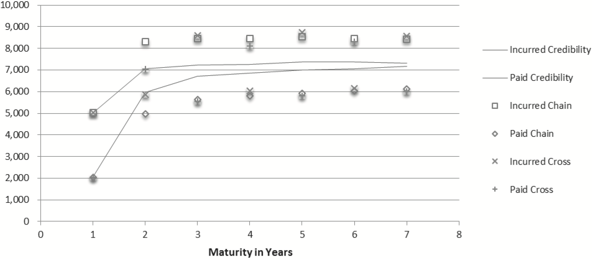
Figure 2 shows how the RC(f, g) paid and incurred indications compare to the solo versions (see section 2 for a definition of a solo model) of the CL and XL for Accident Year 7.

Incurred and paid XL indications crisscross with neither indication converging. On the other hand, the incurred and paid CL indications do not converge but appear separately asymptotic, with the paid well below the incurred indication. The incurred and paid RC indications converge between the indications, as would be expected.

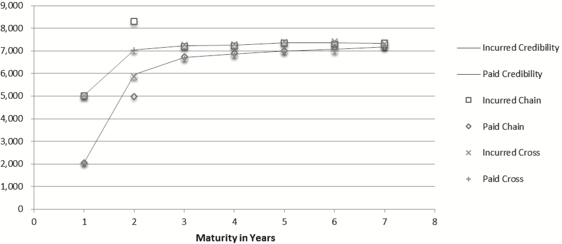
Figure 3 illustrates how the incurred CL and XL submodels give very similar indications after the first indication at age 2. This is because the age 3 CL submodel indication is calculated by multiplying the RC losses at age 2 by the CL factor, and the age 3 XL submodel indication is likewise calculated based on RC losses at age 2. Thus, the maturity 3 indications for both submodels begin from a single pair of RC indications, rather than two pairs of indications—a CL pair and a XL pair.

This practice is consistent with the KPL assumption, i.e., that prior to application of a development factor, loss development up until that point is known. Rather than using a submodel’s prior indication as the input for the next loss indication, the RC indication is assumed to be more accurate, thus the next maturity’s loss development assumptions apply to the more accurate intermediate indication rather than divergent indications.

Table 8 contains RC indications as well as the CL and XL solo indications at age 7 by accident year.

5.4. Comparison of the performance of the MCL with the RC(f, g)

Recalling that the MCL is the weighted sum of the CL and XL indications, an interesting comparison would then be between the MCL and the RC(f, g) indications. To do this comparison, a 10,000 iteration simulation was performed that changed values within the MCL dataset based on the actual triangle distribution.

The simulation design was as follows:

1. The final paid and incurred diagonal of the MCL dataset was unchanged in each iteration.

2. Incurred loss development ratios were assumed to be normally distributed and used to back into the prior diagonals of the triangle, based on the implied mu and sigma of actual development ratios by age.

3. Ratios of incremental paid losses as a percentage of hindsight case reserves^[5] were assumed to be normally distributed with mean and standard deviation of the actual ratios by age.

   a. This amount was capped at 0 and 1.

   b. An additional cap of the minimum future incurred loss was set so that historical paid losses would never decrease.

   c. These assumptions were used to fill out the paid loss triangle starting from the earliest calendar period (the upper left corner of the triangle).

The intention was to build triangles that have “normal” development (paid losses monotonically increase, and incurred losses are non-negative) that could have led to the final diagonal on the MCL triangle from the same set of exposures. Ten thousand such “normal” triangles were generated, using Excel’s random number generator. Eight values were recorded for each iteration, one for each paid and incurred indication for each of the RC(f, g), the MCL, the solo CL and the solo XL models. All the statistics in Table 9 refer to these values.

For both the RC(f, g) and MCL indications, which depend on non-zero proportionality constants, when a constant was calculated as zero, half the constant for the prior age was selected instead.

Table 9 provides summary results of that simulation for the total of all accident year paid and incurred indications at age 7, for the RC(f, g), as well as the MCL, the solo CL, and the solo XL models.

One point that should be made is that the MCL development assumptions were not explicitly used to construct these triangles. However, normal paid and incurred loss development will necessarily have paid and incurred losses that converge to the same ultimate. Therefore, in a general sense, we should still expect the MCL to result in converging indications.

Note that RC(f, g) behaves as desired with incurred and paid averages, minimums and maximums being relatively near those of the CL and XL indications. Furthermore, the average incurred minus paid losses are only $692 with a low standard deviation of only $153. By comparison, the MCL paid, incurred, and incurred minus paid standard deviations are all the highest of the group, with the incurred minus paid standard deviation being higher than either the incurred or the paid standard deviation. The minimums and maximum demonstrate that additional volatility.

Within the simulation detail (not shown) many MCL indications are very close to the RC(f, g) indications, but a number of them also displayed volatility. This limited robustness can limit the MCL’s usefulness with volatile data.

Another point to notice is that the median MCL indications are higher than those of RC(f, g). The average of the median paid and incurred MCL of 32,652 is clearly closer to the CL incurred indication of 33,050 than the paid indication of 30,930. The average of the median paid and incurred RC(f, g) indications is 32,252, closer to the average of the median paid and incurred CL indications of 31,990. Whether this indicates systematic bias of one or both of the indications has not been determined. However, this difference should be duly noted in utilizing both recursive credibility and the MCL.

5.5. Comparison of the accuracy of the RC(f, g), MCL, CL and XL on industry data

Based on the CAS’s “Loss Reserving Data Pulled from NAIC Schedule P” (Meyers 2011) the accuracy of RC(f, g), MCL, CL and XL models on actual data was compared. For each line of business and company, a paid and incurred pair of 7 × 7 grids of loss development data was used. The accident years selected were from 1990 to 1996, and the development lags selected were 1 to 7. Grid pairs that had zero or negative losses in any of these cells were not used. Grid pairs where development had stopped prior to age 7 were also not used. This resulted in an adequate number of grid pairs to consider the following four lines of business.^[6]

1. Private Passenger Auto (PPA)—95 grid pairs

2. Commercial Auto (CmA)—82 grid pairs

3. Workers Compensation (WC)—65 grid pairs

4. Other Liability (OL)—95 grid pairs

For each grid (for a given model and line of business), the upper triangular matrix was developed (completing the square) and the total losses in column 7 (modeled losses) were compared to the total losses in the original grid (actual losses). To allow for differences in loss volume, scaled residuals were calculated as (modeled − actual)/actual^1/2. For comparison of the models, the average scaled residual (ASR) and the root-mean-squared error (RMSE) were calculated. The results are displayed in Table 10.

RC(f, g) appears in most cases to have relatively low magnitude ASRs (a measure of bias) and low RMSE (a measure of uncertainty) for both paid and reported indications for all lines of business when compared to the other models. There are notable parallels between this industry data comparison and the simulation results in section 5.4. For instance, in both the simulation and the industry comparison, RC(f, g) presents a better improvement over the paid indications than the incurred. Furthermore, the incurred CL is a more consistent indicator in the simulation, and appears to have smaller errors in the industry comparison.

On the other hand, the MCL appears to perform slightly better on workers compensation data. Removing a single grid pair (#23108 from the CAS loss reserves data) would make the RMSE for both Paid and Incurred RC(f, g) appear slightly better than Paid and Incurred MCL; however, the ASR for both Paid and Incurred MCL is still smaller than for Paid and Incurred RC(f, g). It is significant that the Paid and Incurred RC(f, g) ASR lies within the range of solo model ASR values for all lines of business. However, for the MCL, either the Paid or the Incurred ASR lies outside the range of the four solo model ASR values for three of the four lines of business. The Incurred MCL PPA ASR = −4.2 < −4.1 < 2.7 < 3.0 < 9.5. The Incurred MCL CmA ASR = −3.9 < −0.8 < 0.9 < 9.2 < 10.5. For Workers Compensation, both the Paid and Incurred ASR lie outside the range of the solo models. Incurred MCL WC ASR < Paid MCL WC ASR = 6.5 < 7.2 < 10 < 10.4 < 12.3. This freedom to “color outside the lines,” which can reduce the stability of the final MCL indications, also allows the MCL to account for downward trend in the development patterns that RC(f, g) by design cannot account for. This demonstrates that RC (f, g) will be more effective with sub-indications having bias of opposite signs, while MCL may provide information when there is unidirectional trend in all development patterns.

The combined simulation results and the industry data results suggest that RC(f, g) does a good job of estimating reasonable paid losses, incurred losses and case reserves. This may, for certain lines of business, result in a less biased estimate than the MCL. However, RC(f, g) will not correct for bias when all submodels are biased in the same direction. In other words, it will not correct for a unidirectional trend in all development patterns (that can be caused by statutory changes in damage awards). For this reason, care must be used in selecting appropriate submodels when using recursive credibility or adjusting triangles to at least remove known shifts and trends in development patterns.

6. Concluding remarks

Some advantages of the recursive credibility framework include:

1. RC allows different assumptions to be weighted by their relevance at different maturities.

2. RC allows a set of assumptions to be considered that would otherwise be summarily dismissed from the actuary’s consideration. Volatile assumptions such as the cross link method may give no clear final ultimate loss indication but may provide valuable additional information within a recursive credibility framework.

3. RC includes a framework for the calculation of the variance of the overall indication, as long as the recursive variance of the underlying submodels is given.

Weaknesses and uncertainties of the RC framework include:

1. The RC framework contains invariant correlation terms.

2. The variance in this framework ignores the fact that when two sets of assumptions reach identical indications, those indications could be seen as having identical variance, and correlation of 1 because their differences from “actual” is identical.

3. The submodels presented here utilize only paid and incurred data. Will the variance of models that utilize exposures, claim counts, or premiums be directly comparable?

Additional research could attempt to address the first two issues. It could seek a more responsive framework to estimate indication-specific variance and covariance terms. It could also seek to allow variance terms to converge when indications converge, and correlation to converge to 1, and it could allow variance to be impacted by clustering.

A follow-up to this paper will attempt to answer the third question by illustrating the use of other loss development and variance assumptions. It will also generalize the recursive credibility framework to N models, and it will give a three-dimensional example.

In conclusion, RC(f, g) offers a significant improvement in stability over the MCL, while still bringing paid and incurred indications closer together. As an outgrowth of the MCL, the recursive credibility framework recognizes the value of recursive credibility-weighting of sub-indications, as opposed to the application of credibility to fully realized solo indications. It is a step toward reserving models that continuously measure the marginal impacts of changes of interdependent variables on one another.

The RC framework significantly reduces the occurrence of unreasonable indications by recognizing and adjusting for the error that credibility weights add to a credibility-weighted indication. To accomplish this, a means of measuring a portion of the parameter error of credibility weights for two sub-indications has been presented.

RC can be used with any sub-indications whose variance can be structured in a manner similar to Mack’s recursive variance structure, where the variance is the sum of two conditional variance terms, the KPL variance and the KDF variance. As the actuarial profession continues to define the variance of its numerous models, recursive credibility can help to reduce model error by allowing more assumptions to enter our estimates and by ensuring that the timing of application of those assumptions is appropriate.

---

Acknowledgments

I would like to thank the individuals who have helped in the journey to publication of this paper:

• To the editors and anonymous peer reviewers of Variance for their feedback and professionalism and for their decision to move forward with the publication of this research.

• To the many actuarial professionals who reviewed and provided feedback on various drafts of this paper, especially Roger Hayne, Joe Walter Rutkowski, Vladimir Shander, Dave Clark and Hsiu-Mei Chang, for their generous donation of time, energy and insight.

• To Dr. Edgar Enochs, for his friendship and his example.

• To Dr. Gerhard Quarg and Dr. Thomas Mack, for their excellent Munich chain ladder model and paper.

I have been educated and encouraged through your work and feedback.

Finally, with the utmost gratitude, I dedicate this paper to my wife, Kazuko.