Multivariate Bühlmann-Straub Credibility Model Applied to Claims Reserving for Correlated Run-off Triangles

undefined

1. Introduction and motivation

A non-life insurance company needs to hold sufficient reserves on its balance sheet in order to meet the future claims payment cashflow. Therefore, given the available information about the past claims payment cash flow and the claims settlement process as well as external knowledge from experts and prior information (e.g., premium, number of contracts, data from similar run-off portfolios, market statistics), the prediction of the outstanding loss liabilities and the quantification of the uncertainties in these predictions is a major task in actuarial practice and science. It is the basis for proving solvency on the one hand and it allows for reliable premium calculations on the other hand (see, e.g., CAS (Casualty Actuarial Society) 2001 and Teugels and Sundt 2004).

In this paper we consider the claims reserving problem in a multivariate context. That is, we consider a portfolio consisting of several correlated run-off portfolios (e.g., subportfolios of certain lines of business) and we apply the multivariate generalization of the well-known credibility model proposed by Bühlmann and Straub (1970) for predicting outstanding loss liabilities. This simultaneous study of several individual run-off triangles is motivated by several important facts (cf. Merz and Wüthrich 2008b).

Since in actuarial practice the conditional mean square error of prediction (MSEP) is the most popular risk measure to quantify the uncertainties in claims reserves, we provide an estimator of the conditional MSEP. Such studies of uncertainties for correlated run-off portfolios are especially crucial in the development of new solvency guidelines for the quantification of risk profiles for different insurance companies. However, they do not provide a complete picture of the uncertainty associated with the predictor of the claims reserves for the total portfolio. This can only be provided by the whole predictive distribution of the claims reserves calculated under very restrictive model assumptions or by applying numerical algorithms such as bootstrapping methods and Markov chain Monte Carlo (MCMC) methods (cf. England and Verrall 2007 and Wüthrich and Merz 2008). However, in practical applications and solvency considerations, estimates for second moments such as the conditional MSEP and its components conditional process variance/estimation error are often sufficient, since in most cases one fits an analytic overall distribution using these first two moments by the method of moments. Moreover, analytic solutions are important because they allow for explicit interpretations in terms of the parameters involved and enable sensitivity analysis with respect to parameter changes.

1.1. Claims reserving methods and credibility theory in a multivariate context

The calculation of the conditional MSEP for the predictor of the ultimate claim for a whole portfolio of several correlated run-off portfolios is more sophisticated than for only one run-off portfolio. Holmberg (1994) was probably the first one to investigate the problem of dependence between run-off portfolios of different lines of business. Later Halliwell (1999) and Quarg and Mack (2004) proposed the first bivariate models which express the dependence between the paid and incurred losses of a single run-off portfolio. Braun (2004) and Merz and Wüthrich (2008a, 2008b) generalized the well-known univariate chain-ladder model of Mack (1993) to the bivariate and the general multivariate case, respectively, by incorporating correlations between different run-off portfolios. They derived an estimate of the conditional MSEP for the predictor of the ultimate claim of the total portfolio. Merz and Wüthrich (2009a) study a special case of the multivariate additive loss reserving model proposed by Hess, Schmidt, and Zocher (2006) and derive an estimate for the conditional MSEP. Moreover, Dahms (2012) presented a general class of models that contains most models mentioned above.

In the present paper we give a credibility approach to the claims reserving problem in a multivariate context. Univariate and multivariate credibility methods are widely used in insurance pricing, but for claims reserving they are less used (though they are also useful in this context). In the claims reserving context univariate credibility methods can, e.g., be found in Benktander (1976), De Vylder (1982), Neuhaus (1992), Mack (2000), Witting (1987), and Gisler and Wüthrich (2008). More recently, Dahms and Happ (forthcoming) presented in a credibility framework a very general class of (multivariate) claims reserving methods, which contains most of the methods mentioned above as special cases. In the present paper we choose a multivariate claims reserving method different from Dahms and Happ (forthcoming) and apply the multivariate generalization of the credibility model of Bühlmann and Straub (1970) to the (multivariate) claims reserving problem.

1.2. Claims development triangle and notation

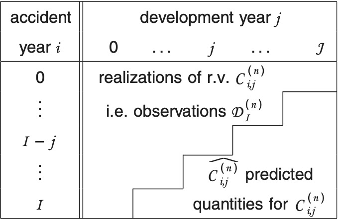
Throughout this paper all random variables are square integrable random variables defined on a common probability space (Ω, ℱ, P). We consider the situation where we have N ≥ 1 portfolios. The associated losses of each portfolio are represented by run-off triangles (claim development triangles). We assume for the reason of simplicity that all run-off triangles are of the same size (the whole theory presented in this paper can be easily generalized to different sizes but the notation then becomes more complicated) and we denote by I (J) the last accident (development) year. The claims development data have the structure shown in Figure 1. Thereby we denote by $X_{i j}^{(i)}$ the incremental claim payments for accident year $i \in\{0, \ldots, I\}$ and development year $j \in\{0, \ldots, J\}$ of run-off portfolio $n \in\{1, \ldots, N\}$.

The cumulative claims payments of triangle n for accident year i up to development year j are denoted by

$$C_{i, j}^{(n)}=\sum_{k=0}^{j} X_{i, k}^{(n)} .$$

For simplicity, we always assume that I = J, i.e., we deal with development triangles (for I ≥ J we have development trapezoids), but all results also hold true under slight modifications for the case I ≥ J.

Usually, at time I we have the sets of observations (σ-algebras)

$$\mathcal{D}_{I}^{(n)}=\sigma\left(C_{i, j}^{(n)} ; i+j \leq I\right) \subseteq \mathcal{F}$$

for all run-off portfolios n ∈ {1, . . . , N}. The total of observation over all run-off portfolios is then given by

$$\mathcal{D}_{I}^{N}=\sigma\left(\bigcup_{n=1}^{N} \mathcal{D}_{I}^{(n)}\right) .$$

For the following derivations it is convenient to write the data of the N run-off portfolios in vector form. Thus we define the N-dimensional random vectors

$$\mathbf{X}_{i, j}=\left(X_{i, j}^{(1)}, \ldots, X_{i, j}^{(N)}\right)^{\prime}$$

and

$$\mathbf{C}_{i, j}=\left(C_{i, j}^{(1)}, \ldots, C_{i, j}^{(N)}\right)^{\prime}$$

of incremental and cumulative claims payments, respectively. The vector of outstanding claims payments for accident year i ∈ {1, . . . , I} is defined by

$$\mathbf{R}_{i}=\left(R_{i}^{(1)}, \ldots, R_{i}^{(N)}\right)^{\prime}=\mathbf{C}_{i, J}-\mathbf{C}_{i,-I i}=\sum_{j=I-i+1}^{J} \mathbf{X}_{i, j} .$$

Furthermore, we define the N-dimensional column vector consisting of ones by 1 = (1, . . . , 1)′ ∈ ℝ^N and the N × N-dimensional identity matrix by I.

2. Multivariate Bühlmann-Straub credibility model

Bayesian methods are often an appropriate tool to combine data with expert opinion, or, in other words, to combine internal data (observations) with external given prior information. However, in most Bayesian models the derivation of the posterior distribution is infeasible and numerical methods such as MCMC or numerical integration have to be applied. Analytical posterior distributions can only be calculated under very restrictive (distributional) model assumptions, for example, if one restricts to distributions from the exponential dispersion family with associated conjugated prior (cf. Bühlmann and Gisler 2005). For an example of this strategy applied in claims reserving we refer to Hashorva, Merz, and Wüthrich (2013). However, in many models it is impossible to express the Bayesian predictor in an analytical closed form. In this case the best we can do is to restrict the class of possible predictors to the class of so-called credibility predictors, which are affine-linear functions of the observations with minimum MSEP; see (2.7). These predictors have the big advantage that prior knowledge and data can be combined for the prediction and that they can be calculated under less restrictive model assumptions than Bayesian predictors. For a detailed introduction and more details on credibility predictors, see Bühlmann and Gisler (2005).

Applied to our multivariate claims reserving problem, this means that we are interested in the predictor of the ultimate claim $\mathbf{C}_{i, J}$ for accident year $i \in$ $\{1, \ldots, I\}$, which is the best affine-linear function of the components of the observations $\mathbf{X}_{i 0}, \ldots, \mathbf{X}_{i, l-i}$ at time $I$ with respect to the MSEP. We study this problem in the framework of the multivariate BühlmannStraub model (cf. Bühlmann and Gisler 2005). In order to formulate the model assumptions of the multivariate Bühlmann-Straub model, we introduce latent random variables $\Theta_i$, which describe the risk characteristics of the different accident years $i=$ $0, \ldots, I$. Moreover, we assume that there are (known) volume measures $\mu_i^{(n)}$ and (unknown) incremental loss development patterns (cash flow patterns) $\left(\gamma_j^{(n)}\right)_{j=0 . \ldots}, \subset \mathbb{R}_{+}$, for the $N$ development triangles $n \in\{1, \ldots, N\}$, such that

$$E\left[X_{i, j}^{(n)}\right]=\gamma_{j}^{(n)} \mu_{i}^{(n)} \tag{2.1}$$

for all i = 0, . . . , I. This leads to the normalized incremental claims payments given by

$$Y_{i, j}^{(n)}=\frac{X_{i,( }^{(n)}}{\gamma_{j}^{(n)} \mu_{i}^{(n)}}$$

for all $i=0, \ldots, I$ and $j=0, \ldots, J$. To shorten notation we define the cumulative loss development patterns $\left(\beta_j^{(n)}\right)_{j=0, \ldots, J} \subset \mathbb{R}_{+}$by

$$\begin{array}{c} \beta_{0}^{(n)}=\gamma_{0}^{(n)}>0 \text { and } \beta_{j}^{(n)}-\beta_{j-1}^{(n)}=\gamma_{j}^{(n)}>0 \\ \text { for } j=1, \ldots, J . \end{array} \tag{2.2}$$

In vector form we have for i = 0, . . . , I and j = 0, . . . , J:

$$\begin{aligned} \pmb{\gamma}_{j} & =\left(\gamma_{j}^{(1)}, \ldots, \gamma_{j}^{(N)}\right)^{\prime} \\ \pmb{\beta}_{j} & =\left(\pmb{\beta}_{j}^{(1)}, \ldots, \pmb{\beta}_{j}^{(N)}\right)^{\prime} \\ \pmb{\mu}_{i} & =\left(\mu_{i}^{(1)}, \ldots, \mu_{i}^{(N)}\right)^{\prime} \\ \mathbf{Y}_{i, j} & =\left(Y_{i, j}^{(1)}, \ldots, Y_{i, j}^{(N)}\right)^{\prime} . \end{aligned}$$

In the following we denote by

$$\mathbf{D}(\mathbf{a})=\left(\begin{array}{ccc} a_{1} & & 0 \\ & \ddots & \\ 0 & & a_{N} \end{array}\right) \text { and } \mathbf{D}(\mathbf{a})^{b}=\left(\begin{array}{ccc} a_{1}^{b} & & 0 \\ & \ddots & \\ 0 & & a_{N}^{b} \end{array}\right)$$

the N × N-diagonal matrices of the N-dimensional vectors a = (a₁, . . . , a_N)′ ∈ ℝ^N and (a^b₁, . . . , a_N^b)′ ∈ ℝ^N for an admissible exponent b ∈ ℝ, respectively. Then we have for the normalized incremental claims

$$\mathbf{Y}_{i, j}=\mathbf{D}\left(\mathbf{w}_{i, j}\right)^{-1} \mathbf{X}_{i, j}, \tag{2.3}$$

where $\mathbf{w}_{i, j}=\left(w_{i, j}^{(1)}, \ldots, w_{i, j}^{(N)}\right)^{\prime}$ with $w_{i, j}^{(n)}=\gamma_j^{(n)} \mu_i^{(n)}$ for all $i=0, \ldots, I, j=0, \ldots, J$ and $n=1, \ldots, N$.

Having this notation the multivariate Bühlmann-Straub model is then given by:

Model Assumptions 2.1 (Multivariate Bühlmann-Straub model)

• Conditionally, given $\Theta_i$, the normalized incremental claims $\mathbf{Y}_{i, 0}, \ldots, \mathbf{Y}_{i, J}$ are independent with

$$E\left[\mathbf{Y}_{i, j} \mid \Theta_{i}\right]=\pmb{\mu}\left(\Theta_{i}\right) \tag{2.4}$$

$$\begin{aligned} \operatorname{Var}\left(\mathbf{Y}_{i, j} \mid \Theta_{i}\right) & =\mathbf{D}\left(\mathbf{w}_{i, j, \xi, \delta}\right)^{-1 / 2} \cdot \Sigma\left(\Theta_{i}\right) \cdot \mathbf{D}\left(\mathbf{w}_{i, j, \xi, \delta}\right)^{-1 / 2} \\ & =\left(\begin{array}{cccc} \frac{\sigma_{1}^{2}\left(\Theta_{i}\right)}{w_{i, j, \xi, \delta}^{(1)}} & 0 & \cdots & 0 \\ 0 & \ddots & & \vdots \\ \vdots & & \ddots & 0 \\ 0 & \cdots & 0 & \frac{\sigma_{N}^{2}\left(\Theta_{i}\right)}{w_{i, j, \xi, \delta}^{(N)}} \end{array}\right) \end{aligned} \tag{2.5}$$

where $w_{i, j, \xi, \delta}^{(n)}=\gamma_j^{(n)^{\xi}} \mu_i^{(n)^\delta}$ with $\xi \in[0,2]$ and $\delta \geq 0$. The matrix $\Sigma\left(\Theta_i\right)=\mathbf{D}\left(\sigma_1^2\left(\Theta_i\right), \ldots, \sigma_N^2\left(\Theta_i\right)\right)$ is the $N \times N$-diagonal matrix of $\left(\sigma_1^2\left(\Theta_i\right), \ldots, \sigma_N^2\left(\Theta_i\right)\right)^{\prime}$.

• The pairs $\left(\Theta_i, \mathbf{Y}_i^{\prime}=\left(\mathbf{Y}_{i, 0}^{\prime}, \ldots, \mathbf{Y}_{i, I}^{\prime}\right)\right)$ for $i=0, \ldots, I$ are independent and the latent variables $\Theta_0, \ldots, \Theta_I$ are identically distributed.

Remarks

• From (2.4) it follows that the normalized incremental claim payments $\mathbf{Y}_{i, j}$ of accident year $i$ are higher or lower than the normalized incremental claim payments $\mathbf{Y}_{k, j}$ of another accident year $k$. This means there are accident years which are systematically better or worse than other ones.

• We assume that the prior volumes $\pmb{\mu}_i=\left(\mu_i^{(1)}, \ldots, \mu_i^{(N)}\right)^{\prime}$ are known and that the incremental loss development pattern $\pmb{\gamma}_j=\left(\gamma_j^{(1)}, \ldots, \gamma_j^{(N)}\right)^{\prime}$ is unknown.

• The weights ξ ∈ [0, 2] and δ > 0 reflect the relation of the (conditional) expected value Equation 2.4 and its variance Equation 2.5. For a discussion and a motivation of choices ξ = 0 and ξ = 1 we refer to Mack (2002). Although the cases ξ = 0 and ξ = 1 can be clearly interpreted, we allow for ξ ∈ [0, 2]. In Section 4 we show how appropriate choices for ξ and δ can be derived.

• The parameter Θ_i tells us whether we have a good or a bad accident year i. For a more detailed explanation in the framework of tariffication and pricing we refer to Bühlmann and Gisler (2005).

• It is straightforward to show that in the case of one-dimensional observations (i.e., N = 1), the assumptions of the (classical) one-dimensional Bühlmann-Straub model are satisfied.

• For the normalized incremental claims and the cumulative claims we obtain

$$E\left[\mathbf{Y}_{i, j}\right]=E\left[\pmb{\mu}\left(\Theta_{i}\right)\right]=\mathbf{1}$$

and, respectively,

$$\begin{aligned} E\left[\mathbf{C}_{i, j} \mid \Theta_{i}\right] & =\mathbf{D}\left(\pmb{\beta}_{j}\right) \mathbf{D}\left(\pmb{\mu}_{i}\right) \pmb{\mu}\left(\Theta_{i}\right) \\ E\left[\mathbf{C}_{i, j}\right] & =\mathbf{D}\left(\pmb{\beta}_{j}\right) \pmb{\mu}_{i} \end{aligned}$$

for all i = 0, . . . , I and j = 0, . . . , J. Moreover, we obtain for the claims reserves

$$\begin{aligned} E\left[\mathbf{R}_{i} \mid \Theta_{i}\right] & =\left(\mathbf{D}\left(\pmb{\beta}_{J}\right)-\mathbf{D}\left(\pmb{\beta}_{I-i}\right)\right) \mathbf{D}\left(\pmb{\mu}_{i}\right) \pmb{\mu}\left(\Theta_{i}\right) \\ E\left[\mathbf{R}_{i}\right] & =\left(\mathbf{D}\left(\pmb{\beta}_{J}\right)-\mathbf{D}\left(\pmb{\beta}_{I-i}\right)\right) \pmb{\mu}_{i} \end{aligned} \tag{2.6}$$

for all i = 1, . . . , I.

In the following we define the MSEP of an N-dimensional predictor $\widehat{\mathbf{X}}=\left(\widehat{X}_{1}, \ldots, \widehat{X}_{N}\right)^{\prime}$ for an N-dimensional random variable X = (X₁, . . . , X_N)′ by

$$\operatorname{msep}_{\mathbf{x}}(\widehat{\mathbf{X}})=\sum_{n=1}^{N} E\left[\left(\widehat{X}_{n}-X_{n}\right)^{2}\right] . \tag{2.7}$$

In the multidimensional credibility theory one looks now for a predictor $\widehat{\pmb{\mu}\left(\Theta_i\right)}$ of $\pmb{\mu}\left(\Theta_i\right)$ that minimizes the MSEP (2.7) among all $N$-dimensional predictors $\widehat{\mathbf{X}}=\left(\widehat{X}_1, \ldots, \widehat{X}_N\right)^{\prime}$ whose components $\widehat{X}_k$ are affine-linear in the components of the N -dimensional observations $\mathbf{X}_{i, 0}, \ldots, \mathbf{X}_{i, I-i}$ with $i=0, \ldots, I$. That is, one has to solve the optimization problem

$$\widehat{\pmb{\mu}\left(\Theta_{i}\right)}=\underset{\left.\widehat{x} \in\left(D_{0}^{\prime}, 1\right)\right)}{\operatorname{argmin}} \operatorname{msep}_{\mu\left(\theta_{i}\right)}(\widehat{\mathbf{X}}),$$

where

$$\begin{array}{l} L\left(\mathcal{D}_{I}^{N}, 1\right) \\ \quad=\left\{\widehat{\mathbf{X}} ; \widehat{X_{k}}=a+\sum_{i=0}^{I} \sum_{j=0}^{I-i} \sum_{n=1}^{N} a_{i, j}^{(n)} X_{i, j}^{(n)} \text { with } a, a_{i, j}^{(n)} \in \mathbb{R}\right\} . \end{array} \tag{2.8}$$

We define the structural parameter matrices

$$\begin{array}{l} S=E\left[\sum\left(\Theta_{i}\right)\right] \\ T=\operatorname{Var}\left(\pmb{\mu}\left(\Theta_{i}\right)\right) \end{array}$$

and obtain:

Theorem 2.2 (Bühlmann-Straub predictor)

Under Model Assumptions 2.1 the optimal affine-linear predictor of µ(Θ_i) is given by

$${\widehat{\pmb{\mu}\left(\Theta_{i}\right)}}^{\text {cred }}=A_{i} \mathbf{K}_{i}+\left(I-A_{i}\right) \mathbf{1} \tag{2.9}$$

for 1 ≤ i ≤ I, where

$$\begin{array}{l} \mathbf{K}_{i}=\left(\sum_{j=0}^{I-i} \frac{\gamma_{j}^{(1)-1}}{\beta_{I-i, j}^{(1)} \mu_{i}^{(1)}} X_{i, j}^{(1)}, \ldots, \sum_{j=0}^{I-i} \frac{\gamma_{j}^{(N)^{\xi-1}}}{\beta_{I-i, j}^{(N)} \mu_{i}^{(N)}} X_{i, j}^{(N)}\right)^{\prime} \\ A_{i}=T\left(T+\mathbf{D}\left(\pmb{\beta}_{I-i, j}\right)^{-1 / 2} \mathbf{D}\left(\pmb{\mu}_{i}\right)^{-\delta / 2} S \mathbf{D}\left(\pmb{\mu}_{i}\right)^{-\delta / 2} \mathbf{D}\left(\pmb{\beta}_{I-i, \xi}\right)^{-1 / 2}\right)^{-1} \\ \pmb{\beta}_{I-i, 5}^{(n)}=\sum_{j=0}^{L-i} \gamma_{j}^{(n)^{5}} \\ \pmb{\beta}_{I-i \xi}=\left(\pmb{\beta}_{I-i \xi}^{(1)}, \ldots, \pmb{\beta}_{I-i, \xi}^{(N)}\right)^{\prime} \end{array}$$

Proof: The normalized incremental claim payments $\mathbf{Y}_{i, j}$ fulfill the model assumptions of the multidimensional Bühlmann-Straub model. Hence, Theorem 2.2 is a direct consequence of Theorem 7.8 in Bühlmann and Gisler (2005).

Remarks

• It is usual to compress the data $\mathbf{X}_{i, 0}, \ldots, \mathbf{X}_{i, I-i}$ in an appropriate manner so that we have a single observation vector $\mathbf{K}_i$, which has the same dimension as $\pmb{\mu}\left(\Theta_i\right)$:

$$\begin{array}{l} \mathbf{K}_{i}=\left(\sum_{j=0}^{I-i} \frac{w_{i, j, \xi, \delta}^{(1)}}{\sum_{j=0}^{I-i} w_{i, j, \xi, \delta}^{(1)}} Y_{i, j}^{(1)}, \ldots, \sum_{j=0}^{I-i} \frac{w_{i, j, \delta, \delta}^{(N)}}{\sum_{j=0}^{I-i} w_{i, j, \xi, \delta}^{(N)}} Y_{i, j}^{(N)}\right)^{\prime} \\ =\left(\sum_{j=0}^{I-i} \frac{\pmb{\gamma}_{j}^{(1)} \pmb{\beta}_{I-i, \xi}^{(1)} \pmb{\mu}_{i}^{(1)}}{(1)} X_{i, j}^{(1)}, \ldots, \sum_{j=0}^{I-i} \frac{\pmb{\gamma}_{j}^{(N)^{\xi-1}}}{\pmb{\beta}_{I-i, j}^{(N)} \pmb{\mu}_{i}^{(N)}} X_{i, j}^{(N)}\right)^{\prime} . \end{array}$$

Observe that the compressed vector $\mathbf{K}_i$ only depends on the observations of accident year i. This is a consequence of the independence assumption between different accident years. Vector $\mathbf{K}_i$ contains all information which is relevant for accident year i, and its n-th component is defined as the weighted average of the normalized incremental claims $Y_{i, j}^{(n)}$ over all observed development years $j=0, \ldots, I-i$.

• Note that

$$\begin{array}{l} \mathbf{D}\left(\pmb{\beta}_{I-i, \xi}\right)^{-1 / 2} \mathbf{D}\left(\pmb{\mu}_{i}\right)^{-\delta / 2} S \mathbf{D}\left(\pmb{\mu}_{i}\right)^{-8 / 2} \mathbf{D}\left(\pmb{\beta}_{I-i \xi}\right)^{-1 / 2} \end{array}$$

where $\sigma_n^2=E\left[\sigma_n^2\left(\Theta_i\right)\right]$ for $n=1, \ldots, N$.

• Credibility predictor (2.9) is unbiased for the prior mean $E\left[\pmb{\mu}\left(\Theta_i\right)\right]=\mathbf{1}$.

• In the case of one-dimensional observations and ξ = 1 predictor (2.9) reduces to the one-dimensional credibility predictor applied to the claims reserving problem (cf. Wüthrich and Merz 2008).

To obtain a predictor for the outstanding claim payments we have to determine an estimator for the parameter $\pmb{\gamma}_j$ and $\pmb{\beta}_j$, respectively. An unbiased estimator for $\pmb{\gamma}_j$ is given by

$$\hat{\pmb{\gamma}}_{j}=\mathbf{D}\left(\sum_{i=0}^{I-j} \pmb{\mu}_{i}\right)^{-1} \sum_{i=0}^{I-j} \mathbf{X}_{i, j} \tag{2.10}$$

for all j = 0, . . . , J. Thus the estimator

$$\hat{\pmb{\beta}}_{j}=\sum_{k=0}^{i} \hat{\pmb{\gamma}}_{k} \tag{2.11}$$

is an unbiased estimator for $\pmb{\beta}_j$ for all $j=0, \ldots, J$. This leads to the following predictor:

Predictor 2.3 Under Model Assumptions 2.1 we have the following predictors for the ultimate claims

$${\widehat{\mathbf{C}_{i, J}}}^{\text {cred }}=\mathbf{C}_{i,-i-i}+\mathbf{D}\left(\hat{\pmb{\beta}}_{J}-\hat{\pmb{\beta}}_{I-i}\right) \mathbf{D}\left(\pmb{\mu}_{i}\right) \widehat{\pmb{\mu}\left(\pmb{\Theta}_{i}\right)}{\mathstrut}^{\text{cred}} \tag{2.12}$$

for 1 ≤ i ≤ I.

For the numerical calculation of the predictor (2.12) we have to estimate the structure parameter matrices S and T. This will be done in Section 4.

Under Model Assumptions 2.1 the predicted outstanding claim payments are given by

$$\begin{aligned} \widehat{\mathbf{R}}_{i}^{\text {cred }} & =\left({\widehat{R_{i}^{(1)}}}_{\text {(red }}, \ldots,{\widehat{\pmb{R}_{i}^{(N)}}}^{\text {cred }}\right)^{\prime} \\ & \left.=\mathbf{D}\left(\hat{\pmb{\beta}}_{j}-\hat{\pmb{\beta}}_{I-i}\right) \mathbf{D}\left(\pmb{\mu}_{i}\right) \widehat{\pmb{\mu}\left(\Theta_{i}\right.}\right)^{\text {cred }} \end{aligned} \tag{2.13}$$

for 1 ≤ i ≤ I.

For the derivation of the (conditional) MSEP in the next section the following lemma on the quadratic loss matrices of the multidimensional credibility predictors will be used:

Lemma 2.4 In the multidimensional Bühlmann-Straub Model (2.1), the quadratic loss matrices for the credibility predictors are given by

$$\small{ \left.\left.E\left[\left(\widehat{\pmb{\mu ( \Theta}} \widehat{\Theta}_{i}\right)^{\text {cred }}-\pmb{\mu}\left(\Theta_{i}\right)\right) \cdot\left(\widehat{\pmb{\mu}\left(\Theta_{i}\right.}\right)^{\text {cred }}-\pmb{\mu}\left(\Theta_{i}\right)\right)^{\prime}\right]=\left(I-A_{i}\right) T \tag{2.14}}$$

for 1 ≤ i ≤ I.

Proof: The stated quadratic loss of the credibility predictor ${\widehat{\pmb{\mu}\left(\Theta_{i}\right)}}^{\mathrm{cred}}$ in Lemma 2.4 is a direct consequence of Theorem 7.5 in Bühlmann and Gisler (2005).

3. Conditional mean square error of prediction

In the last section we have provided predictors for the ultimate claims and the outstanding claim payments. In this section we quantify the prediction uncertainty of these predictions for single and aggregated accident years in terms of second moments. More precisely, our goal is to derive an estimate for the conditional MSEP of the predicted outstanding claim payments for single as well as aggregated accident years

$$\sum_{n=1}^{N} \widehat{R_{i}^{(n) d}}=\mathbf{1}^{\prime} \widehat{\mathbf{R}}_{i}^{\text {cred }} \quad \sum_{i=1}^{I} \sum_{n=1}^{N} \widehat{R_{i}^{(n) e d ~}}=\sum_{i=1}^{I} \mathbf{1}^{\prime} \widehat{\mathbf{R}}_{i}^{\text {cred }} .$$

We derive these estimators under the assumption that all parameters in the Bühlmann-Straub credibility predictor ${\widehat{\pmb{\mu}\left(\Theta_{i}\right)}}^{\mathrm{cred}}$ in ${\widehat{R_{i}^{(n)}}}^{\text {cred }}$ are known. Afterwards, all parameters are replaced by their estimates. This approach is generally applied for such kind of questions and is known as “empirical credibility approach.”

3.1. Single accident years

The conditional MSEP for a single year $i \in\{1, \ldots, I\}$, given $\mathcal{D}_I^N$, is defined by

$$\begin{array}{l} \operatorname{msep}_{\sum_{n}^{R_{i}^{(n)} D_{i}^{N}}}\left(\sum_{n=1}^{N}{\widehat{R_{i}^{(n)}}}^{\text {cred }}\right)\\ =E\left[\left(\sum_{n=1}^{N}{\widehat{R_{i}^{(n)}}}^{\text {cred }}-\sum_{n=1}^{N} R_{i}^{(n)}\right)^{2} \mid \mathcal{D}_{I}^{N}\right] \\ =\mathbf{1}^{\prime} E\left[\left(\widehat{\mathbf{R}}_{i}^{\text {cred }}-\mathbf{R}_{i}\right)\left(\widehat{\mathbf{R}}_{i}^{\text {cred }}-\mathbf{R}_{i}\right)^{\prime} \mid \mathcal{D}_{I}^{N}\right] \mathbf{1} . \end{array} \tag{3.1}$$

It can be decomposed into conditional process variance and conditional estimation error:

$$\begin{array}{l} \operatorname{msep}_{\sum_{n}^{R_{i}^{(n)} \mid D_{i}^{N}}}\left(\sum_{n=1}^{N}{\widehat{\mathbf{R}_{i}^{(n)}}}^{\text {cred }}\right)=\underbrace{\mathbf{1}^{\prime} \operatorname{Var}\left(\mathbf{R}_{i} \mid \mathcal{D}_{I}^{N}\right) \mathbf{1}}_{\text {conditional process variance }} \\ +\underbrace{\left.\mathbf{1}^{\prime}\left(\widehat{\mathbf{R}}_{i}^{\text {cred }}-E\left[\mathbf{R}_{i} \mid \mathcal{D}_{I}^{N}\right]\right)\left(\widehat{\mathbf{R}}_{i}^{\text {cred }}-E\left[\mathbf{R}_{i} \mid \mathcal{D}_{I}^{N}\right]\right)\right)^{\prime}}_{\text {condional estimaion error }} . \end{array} \tag{3.2}$$

Note that for this decoupling we use the fact that $\widehat{\mathbf{R}}_i^{\text {cred }}$ is known/observable at time $I$ (i.e., $\widehat{\mathbf{R}}_i^{\text {cred }}$ is $\mathcal{D}_I^N$-measurable). For the conditional process variance we obtain the following result:

Lemma 3.1 Under Model Assumptions 2.1 the conditional process variance for a single accident year i ∈ {1, . . . , I} is given by

$$\begin{array}{l} \mathbf{1}^{\prime} \operatorname{Var}\left(\mathbf{R}_{i} \mid \mathcal{D}_{I}^{N}\right) \mathbf{1} \\ =\mathbf{1}^{\prime} \mathbf{D}\left(\pmb{\mu}_{i}\right)^{2-8} E\left[\Sigma\left(\Theta_{i}\right) \mid \mathcal{D}_{I}^{N}\right] \sum_{j=I-i+1}^{J} \mathbf{D}\left(\pmb{\gamma}_{j}\right)^{2-\xi} \mathbf{1} \\ \quad+\mathbf{1}^{\prime} \mathbf{D}\left(\pmb{\beta}_{J}-\pmb{\beta}_{I-i}\right) \mathbf{D}\left(\pmb{\mu}_{i}\right) \operatorname{Var}\left(\pmb{\mu}\left(\Theta_{i}\right) \mid \mathcal{D}_{I}^{N}\right) \\ \quad \mathbf{D}\left(\pmb{\beta}_{J}-\pmb{\beta}_{I-i}\right) \mathbf{D}\left(\pmb{\mu}_{i}\right) \mathbf{1} \end{array} \tag{3.3}$$

Proof. See Appendix.

The conditional process variance $\mathbf{1}^{\prime} \operatorname{Var}\left(\mathbf{R}_i \mid \mathcal{D}_I^N\right)$ originates from stochastic movements of $\mathbf{R}_i$. If we approximate $E\left[\Sigma\left(\Theta_i\right) \mid \mathcal{D}_I^N\right]$ and $\operatorname{Var}\left(\pmb{\mu}\left(\Theta_i\right) \mid \mathcal{D}_I^N\right)$ by $S$ and $T$, respectively, and if we replace the development pattern $\pmb{\gamma}_j$ as well as the structure parameters $S$ and $T$ by their corresponding estimators (see Section 4) we obtain the following estimator of the conditional process variance for a single accident year:

Estimator 3.2 (Conditional process variance for single accident years)

Under Model Assumptions 2.1 we have the following estimator for the conditional process variance of a single accident year i ∈ {1, . . . , I}:

$$\begin{aligned} \mathbf{1}^{\prime} \widehat{\operatorname{Var}}\left(\mathbf{R}_{i} \mid \mathcal{D}_{I}^{N}\right) \mathbf{1}= & \mathbf{1}^{\prime} \mathbf{D}\left(\pmb{\mu}_{i}\right)^{2-8} \hat{S} \sum_{j=I-i+1}^{J} \mathbf{D}\left(\hat{\pmb{\gamma}}_{j}\right)^{2-\xi} \mathbf{1} \\ & +\mathbf{1}^{\prime} \mathbf{D}\left(\widehat{\pmb{\beta}}_{J}-\widehat{\pmb{\beta}}_{I-i}\right) \mathbf{D}\left(\pmb{\mu}_{i}\right) \times \\ & \widehat{T} \mathbf{D}\left(\widehat{\pmb{\beta}}_{J}-\widehat{\pmb{\beta}}_{I-i}\right) \mathbf{D}\left(\pmb{\mu}_{i}\right) \mathbf{1} \end{aligned} \tag{3.4}$$

(see Section 4 for estimates of the structure parameter matrices S and T.)

The conditional estimation error in (3.2) reflects the uncertainty in the prediction of the conditional expectation (mean value) $E\left[\mathbf{R}_i \mid \mathcal{D}_I^N\right]$ by $\widehat{R_i^{(n)}}$. After some calculations (see Appendix) and replacing the unknown parameters by their estimates (see Section 4) we obtain the following result:

Estimator 3.3 (Conditional estimation error for single accident years)

Under Model Assumptions 2.1 we have the following estimator for the conditional estimation error of a single accident year i ∈ {1, . . . , I}:

$$\begin{array}{l} \mathbf{1}^{\prime} \widehat{\operatorname{Var}}\left(\widehat{\mathbf{R}}_{i}^{\text {cred }} \mid \mathcal{D}_{I}^{N}\right) \mathbf{1} \\ =-\mathbf{1} \mathbf{D}\left(\pmb{\mu}_{i}\right) \mathbf{D}\left(\hat{\pmb{\beta}}_{J}-\widehat{\pmb{\beta}}_{I-i}\right) \hat{A}_{i} \hat{T} \mathbf{D}\left(\hat{\pmb{\beta}}_{J}-\widehat{\pmb{\beta}}_{I-i}\right) \mathbf{D}\left(\pmb{\mu}_{i}\right) \mathbf{1} \\ +\mathbf{1}^{\prime} \mathbf{D}\left(\pmb{\mu}_{i}\right) \mathbf{D}\left({\widehat{\left.\pmb{\mu}_{\left(\Theta_{i}\right.}\right)}}^{\text {cred }}\right) \widehat{\operatorname{Var}}\left(\hat{\pmb{\beta}}_{J}-\widehat{\pmb{\beta}}_{I-i}\right) \times \\ \mathbf{D}\left({\widehat{\left.\overline{\pmb{\mu}\left(\Theta_{i}\right.}\right)}}^{\text {cred }}\right) \mathbf{D}\left(\pmb{\mu}_{i}\right) \mathbf{1}, \end{array} \tag{3.5}$$

where

$$\begin{array}{l} \widehat{\operatorname{Var}}\left(\hat{\pmb{\beta}}_{J}-\hat{\pmb{\beta}}_{I-i}\right) \\ =\sum_{j, l>I-i} \mathbf{D}\left(\sum_{m=0}^{I-j} \pmb{\mu}_{m}\right)^{-1}\left[\delta_{j l} \mathbf{D}\left(\hat{\pmb{\gamma}}_{j}\right)^{2-\xi} \cdot \sum_{k=0}^{I-j} \mathbf{D}\left(\pmb{\mu}_{k}\right)^{2-8} \hat{S}\right. \\ \left.\quad+\mathbf{D}\left(\hat{\pmb{\gamma}}_{j}\right) \sum_{k=0}^{I-\max \{j, l]} \mathbf{D}\left(\pmb{\mu}_{k}\right) \hat{T} \mathbf{D}\left(\pmb{\mu}_{k}\right) \mathbf{D}\left(\hat{\pmb{\gamma}}_{l}\right)\right] \mathbf{D}\left(\sum_{m=0}^{I-j} \pmb{\mu}_{m}\right)^{-1} \end{array} \tag{3.6}$$

$${\widehat{\widehat{\pmb{\mu}\left(\Theta_{i}\right)}}}^{\text {cred }}=\widehat{A}_{i} \widehat{\mathbf{K}}_{i}+\left(I-\widehat{A}_{i}\right) \mathbf{1} \tag{3.7}$$

$$\widehat{\mathbf{K}}_i=\left(\sum_{j=0}^{l-1} \frac{\left(\hat{\gamma}_j^{(1)}\right)^{\xi-1}}{\hat{\beta}_{l-i j}^{(1)} \pmb{\mu}_i^{(1)}} X_{i j}^{(1)}, \ldots, \sum_{j=0}^{t-i} \frac{\left(\hat{\gamma}_j^{(N)}\right)^{\xi-1}}{\hat{\pmb{\beta}}_{l-i<k}^{(N)} \mu_i^{(N)}} X_{i j j}^{(N)}\right)^{\prime}\tag{3.8}$$

$$\widehat{A}_{i}=\widehat{T}\left(\widehat{T}+\mathbf{D}\left(\hat{\pmb{\beta}}_{I-i, \xi}\right)^{-1 / 2} \mathbf{D}\left(\pmb{\mu}_{i}\right)^{-\delta / 2} \hat{S} \mathbf{D}\left(\pmb{\mu}_{i}\right)^{-\delta / 2} \mathbf{D}\left(\widehat{\pmb{\beta}}_{I-i, \xi}\right)^{-1 / 2}\right)^{-1} \tag{3.9}$$

and $\delta_{j l}=1$ if $j=l$ and $\delta_{j l}=0$ else (see Section 4 for estimates of the structure parameter matrices $S$ and $T$.)

Combining Estimators 3.2 and 3.3 leads to the following estimator for the conditional MSEP of the predicted outstanding claim payments for a single accident year:

Estimator 3.4 (Conditional MSEP for single accident years)

Under Model Assumptions 2.1 we have the following estimator for the conditional MSEP of a single accident year i ∈ {1, . . . , I}:

$$\begin{array}{l} =\mathbf{1}^{\prime} \widehat{\operatorname{Var}}\left(\mathbf{R}_{i} \mid \mathcal{D}_{I}^{N}\right) \mathbf{1}+\mathbf{1}^{\prime} \widehat{\operatorname{Var}}\left(\widehat{\mathbf{R}}_{i}^{\text {cred }} \mid \mathcal{D}_{I}^{N}\right) \mathbf{1}, \end{array} \tag{3.10}$$

where the two terms on the right-hand side of (3.10) are given by (3.4) and (3.5), respectively.

Remarks

• Predictor (3.7) is the so-called empirical credibility predictor, which results from the credibility predictor (2.9) by replacing the structural parameters by their estimates.

• For N = 1 (i.e., only one run-off portfolio) estimator (3.10) leads to the following estimator

$$\begin{array}{l} \widehat{\operatorname{msep}}_{R_{i, 1} \mathcal{D}_{l}}\left(\widehat{R}_{i}^{\text {cred }}\right)=\underbrace{\mu_{i}^{2-\delta} \hat{S} \sum_{j=I-l+1}^{J} \hat{\gamma}_{j}^{2-\xi}+\mu_{i}^{2}\left(\sum_{j=l i+1}^{J} \hat{\gamma}_{j}\right)^{2} \hat{T}}_{\text {conditional l process variance }} \\ \underbrace{\left.-\mu_{i}^{2}\left(\sum_{j=I-i+1}^{J} \hat{\gamma}_{j}\right)^{2} \widehat{A}_{i} \widehat{T}+\mu_{i}^{2}\left(\widehat{\widehat{\mu\left(\Theta_{i}\right.}}\right)^{\text {cred }}\right)^{2} \widehat{\operatorname{Var}}\left(\sum_{j=I-i+1}^{J} \hat{\gamma}_{j}\right)}_{\text {conditional etimation error }}, \end{array} \tag{3.11}$$

where

$$\begin{array}{l} \widehat{\operatorname{Var}}\left(\sum_{j=I-i+1}^{J} \hat{\gamma}_{j}\right)=\sum_{j, l l \mid-i}\left(\sum_{m=0}^{I-j} \mu_{m}\right)^{-1}\left(\sum_{m=0}^{I-l} \mu_{m}\right)^{-1} \\ {\left[\delta_{j i} \hat{\gamma}_{j}^{2-\xi} \sum_{k=0}^{I-j} \mu_{k}^{2-\xi} \hat{S}+\hat{\gamma}_{j} \hat{\gamma}_{l} \hat{T}^{I-\max (i, i)} \sum_{k=0}^{2} \mu_{k}^{2}\right]} \end{array} \tag{3.12}$$

and

$${\widehat{\overline{\mu\left(G\left(\Theta_{i}\right)\right.}}}^{\text {red }}=\widehat{A}_{i} \widehat{K}_{i}+\left(1-\widehat{A}_{i}\right) 1$$

with

$$\widehat{K}_{i}=\frac{\sum_{j=0}^{I-i} \hat{\gamma}_{j}^{\xi-1}}{\hat{\beta}_{I-i, \xi} \mu_{i}} X_{i, j} \quad \text { and } \quad \hat{A}_{i}=\frac{\hat{\beta}_{I-i, \xi}}{\hat{\beta}_{I-i, \xi}+\frac{\hat{S}}{\mu_{i}^{\delta} \hat{T}}} .$$

3.2. Aggregated accident years

At first we consider the case of two different accident years $1 \leq i<k \leq I$. We have to be careful if we aggregate the estimators $\widehat{\mathbf{R}}_i^{\text {cred }}$ and $\widehat{\mathbf{R}}_k^{\text {cred }}$ because they use the same observations for estimating the parameters $\pmb{\gamma}_j$ and $\pmb{\beta}_j$, respectively. Therefore, they are not independent. We define the conditional MSEP of two aggregated accident years $i$ and $k$ by

$$\begin{array}{l} \operatorname{msep}_{\sum_{n}^{\left.R_{i}^{(n)}\right)}} \sum_{n_{k}^{R_{k}^{(n)} \mid D_{l}^{N}}}\left(\sum_{n=1}^{N}{\widehat{R_{i}^{(n)}}}^{\text {cred }}+\sum_{n=1}^{N}{\widehat{R_{k}^{(n)}}}^{c \text { cred }}\right) \\ \quad=E\left[\left(\sum_{n=1}^{N}\left({\widehat{R_{i}^{(n)}}}^{\text {cred }}+{\widehat{R_{k}^{(n)}}}^{\text {cred }}\right)-\sum_{n=1}^{N}\left(R_{i}^{(n)}+R_{k}^{(n)}\right)\right)^{2} \mid \mathcal{D}_{I}^{N}\right] \end{array}$$

As for a single accident year we have the decomposition

$$\begin{array}{l} \operatorname{msep}_{\sum_{n}^{R_{i}^{(n)}}+\sum_{n}^{R_{k}^{(n)} \mid \mathcal{D}_{I}^{N}}}\left(\sum_{n=1}^{N}{\widehat{R_{i}^{(n)}}}^{\text {cred }}+\sum_{n=1}^{N}{\widehat{R_{k}^{(n)}}}^{\text {cred }}\right) \\ =\mathbf{1}^{\prime} \operatorname{Var}\left(\mathbf{R}_{i}+\mathbf{R}_{k} \mid \mathcal{D}_{I}^{N}\right) \mathbf{1} \\ \quad+\mathbf{1}^{\prime}\left(\widehat{\mathbf{R}}_{i}^{\text {cred }}+\widehat{\mathbf{R}}_{k}^{\text {cred }}-E\left[\mathbf{R}_{i}+\mathbf{R}_{k} \mid \mathcal{D}_{I}^{N}\right]\right) \times \\ \quad\left(\widehat{\mathbf{R}}_{i}^{\text {cred }}+\widehat{\mathbf{R}}_{k}^{\text {cred }}-E\left[\mathbf{R}_{i}+\mathbf{R}_{k} \mid \mathcal{D}_{I}^{N}\right]\right)^{\prime} \mathbf{1} \end{array}$$

Using the independence of different accident years, the conditional MSEP of two aggregated accident years can be represented as follows:

$$\begin{array}{l} \operatorname{msep}_{\sum_{n}^{R_{i}^{(n)}}+\sum_{n} R_{k}^{(n)} \mathcal{D}_{i}^{N}}\left(\sum_{n=1}^{N}{\widehat{R_{i}^{(n)}}}^{\text {cred }}+\sum_{n=1}^{N}{\widehat{R_{k}^{(n)}}}^{\text {cred }}\right) \\ =\operatorname{msep}_{\sum_{n} R_{i}^{(n)} \mid D_{i}^{N}}\left(\sum_{n=1}^{N}{\widehat{R_{i}^{(n)}}}^{c \text { cred }}\right)+\operatorname{msep}_{\sum_{n}^{R_{k}^{(n)} \mid D_{i}^{N}}}\left(\sum_{n=1}^{N}{\widehat{R_{k}^{(n)}}}^{(r e r d}\right) \\ +2 \cdot \mathbf{1}^{\prime}\left(\widehat{\mathbf{R}}_{i}^{\text {cred }}-E\left[\mathbf{R}_{i} \mid \mathcal{D}_{I}^{N}\right]\right)\left(\widehat{\mathbf{R}}_{k}^{\text {cred }}-E\left[\mathbf{R}_{k} \mid \mathcal{D}_{I}^{N}\right]\right)^{\prime} \mathbf{1} . \end{array} \tag{3.13}$$

Since we have already derived an estimator for the first and second term on the right-hand side of (3.13) (cf. Estimator 3.4) we only have to derive an estimator for the third term to obtain an estimator for the MSEP (3.13). After some calculations (see Appendix) and replacing the parameters by their estimates (see Section 4) we obtain for the third term the following estimator:

$$\begin{array}{l} 2 \cdot \mathbf{1}^{\prime} \mathbf{D}\left(\pmb{\mu}_{i}\right) \mathbf{D}\left({\widehat{\overline{\pmb{\mu}\left(\Theta_{i}\right.}}}^{\text {cred }}\right) \widehat{\operatorname{Cov}}\left(\hat{\pmb{\beta}}_{J}-\hat{\pmb{\beta}}_{I-i}, \hat{\pmb{\beta}}_{J}-\hat{\pmb{\beta}}_{I-k}\right) \times \\ \mathbf{D}\left({\widehat{\overline{\pmb{\mu}\left(\pmb{\Theta}_{k}\right.}}}^{\text {cred }}\right) \mathbf{D}\left(\pmb{\mu}_{k}\right) 1, \end{array} \tag{3.14}$$

where

$$\begin{array}{l} \widehat{\operatorname{Cov}}\left(\hat{\pmb{\beta}}_{J}-\hat{\pmb{\beta}}_{I-i}, \hat{\pmb{\beta}}_{I}-\hat{\pmb{\beta}}_{I-k}\right) \\ =\widehat{\operatorname{Var}}\left(\hat{\pmb{\beta}}_{J}-\hat{\pmb{\beta}}_{I-i}\right)+\sum_{\substack{-i<i j \\ I-k<l-i}} \mathbf{D}\left(\sum_{m=0}^{I-j} \pmb{\mu}_{m}\right)^{-1} \mathbf{D}\left(\hat{\gamma}_{J}\right) \times \\ \sum_{s=0}^{I-\max \{j i l\}} \mathbf{D}\left(\pmb{\mu}_{s}\right) \hat{T} \mathbf{D}\left(\pmb{\mu}_{s}\right) \mathbf{D}\left(\hat{\gamma}_{l}\right) \mathbf{D}\left(\sum_{m=0}^{I-l} \pmb{\mu}_{m}\right)^{-1} \end{array} \tag{3.15}$$

and $\widehat{\operatorname{Var}}\left(\hat{\pmb{\beta}}_{J}-\hat{\pmb{\beta}}_{I-i}\right)$ is given by (3.6). For more details on the derivation, see the Appendix.

For the generalization on more than two accident years we use the decomposition

$$\begin{array}{l} +2 \sum_{1 s i<k s I} \cdot 1^{\prime}\left(\widehat{\mathbf{R}}_{i}^{c r e d}-E\left[\mathbf{R}_{i} \mid \mathcal{D}_{I}^{N}\right]\right)\left(\widehat{\mathbf{R}}_{k}^{c r e d}-E\left[\mathbf{R}_{k} \mid \mathcal{D}_{I}^{N}\right]\right)^{\prime} 1 . \end{array}$$

This leads to the following estimator for the conditional MSEP of aggregated years:

Estimator 3.5 (Conditional MSEP for aggregated accident years)

Under Model Assumptions 2.1 we have the following estimator for the conditional MSEP for aggregated accident years:

$$\begin{array}{l} \widehat{\mathrm{msep}} \sum_{i} \sum_{n}^{\left.R_{i}^{(n)}\right)_{l}^{N}}\left(\sum_{i=1}^{L} \sum_{n=1}^{N} \widehat{R_{i}^{(n)}}{\mathstrut}^{\text {cred }}\right) \\ =\sum_{i=1}^{I} \widehat{\operatorname{msep}} \sum_{n_{i}^{(n)} \mid D_{i}^{N}}\left(\sum_{n=1}^{N}{\widehat{R_{i}^{(n)}}}^{\text {cred }}\right) \\ +2 \sum_{1 \leq i<k s} \mathbf{1}^{\prime} \mathbf{D}\left(\mu_{i}\right) \mathbf{D}\left({\hat{{\pmb{\mu}\left(\Theta_{i}\right)}^{c}}}^{\text {cred }}\right) \\ \widehat{\operatorname{Cov}}\left(\hat{\pmb{\beta}}_{s}-\hat{\pmb{\beta}}_{I-i}, \hat{\pmb{\beta}}_{s}-\hat{\pmb{\beta}}_{I-k}\right) \mathbf{D}\left({\widehat{\pmb{\mu}\left(\pmb{\Theta}_{k}\right)}}^{\text {cred }}\right) \mathbf{D}\left(\pmb{\mu}_{k}\right) \mathbf{1}, \end{array} \tag{3.16}$$

with $\widehat{\operatorname{Cov}}\left(\hat{\pmb{\beta}}_{s}-\hat{\pmb{\beta}}_{I-i}, \hat{\pmb{\beta}}_{I}-\hat{\pmb{\beta}}_{I-k}\right)$ given by (3.15).

Remark

For N = 1 (i.e., only one run-off portfolio) Estimator 3.5 leads to the estimator

$$\begin{array}{l} \widehat{\operatorname{msep}} \sum_{i_{i}^{R_{i} \mid D_{i}^{N}}}\left(\sum_{i=1}^{I} \widehat{R}_{i}^{\text {cred }}\right)=\sum_{i=1}^{I} \widehat{\operatorname{msep}}_{R_{i} \mid D_{l}^{N}}\left(\widehat{R}_{i}^{\text {cred }}\right) \\ +2 \sum_{1 s i<k I} \mu_{i} \mu_{k}{\widehat{\widehat{\mu\left(\Theta_{i}\right)}}}^{\text {cred }}{\widehat{\mu\left(\Theta_{k}\right)}}^{\text {cred }} \widehat{\operatorname{Cov}}\left(\sum_{j=I-i+1}^{J} \hat{\gamma}_{j}, \sum_{j=I-k+1}^{J} \hat{\gamma}_{j}\right), \end{array}$$

where $\widehat{\operatorname{msep}}_{\mathrm{R}_{\mathrm{R} \mid D_{i}^{N}}}\left(\widehat{R}_{i}^{\text {cred }}\right)$ is given in (3.11) and

$$\begin{array}{l} \widehat{\operatorname{Cov}}\left(\sum_{j=I-i+1}^{J} \hat{\gamma}_{j}, \sum_{j=I-k+1}^{J} \hat{\gamma}_{j}\right)=\widehat{\operatorname{Var}}\left(\sum_{j=I-i+1}^{J} \hat{\gamma}_{j}\right) \\ \quad+\sum_{\substack{I-i<j \\ I-k<\leq I-i}}\left(\sum_{m=0}^{I-j} \mu_{m}\right)^{-1}\left(\sum_{m=0}^{I-l} \mu_{m}\right)^{-1} \hat{\gamma}_{j} \hat{\gamma}_{l} \widehat{T}^{I-\max \{j, l]} \sum_{s=0}^{2}, \end{array}$$

with $\widehat{\operatorname{Var}}\left(\sum_{j=I-i+1}^{J} \hat{\gamma}_{j}\right)$ given in (26).

4. Parameter estimation

The estimators of the development pattern $\pmb{\gamma}_j$ and $\pmb{\beta}_j$ are given in (2.10) and (2.11). In this section we first give estimators for the structure parameter matrices $S$ and $T$ for known $\pmb{\gamma}_j$ and $\pmb{\beta}_j$. Then, we replace $\pmb{\gamma}_i$ and $\pmb{\beta}_j$ by their estimators (2.10) and (2.11) in order to get the final estimators. Under Model Assumptions 2.1 $S$ is a diagonal matrix, where the diagonal elements $\sigma_n^2=E\left[\sigma_n^2\left(\Theta_i\right)\right], n=1, \ldots, N$ can be estimated by (see Bühlmann and Gisler 2005):

$$\hat{\mathbf{\sigma}}_{n}^{2}=\frac{1}{I} \sum_{i=0}^{I-1} \frac{1}{I-i} \sum_{j=0}^{I-1} \gamma_{j}^{\xi^{(n)}} \pmb{\mu}_{i}^{\delta^{(n)}}\left(\frac{X_{i, j}^{(n)}}{\pmb{\gamma}_{j}^{(n)} \pmb{\mu}_{i}^{(n)}}-\pmb{K}_{i}^{(n)}\right)^{2} . \tag{4.1}$$

We replace $\gamma_{j}^{(n)}$ by $\hat{\gamma}_{j}^{(n)}$ in (4.1) and thus the estimator of the structure parameter matrix S is given by

$$\hat{S}=\left(\begin{array}{cccc} \hat{\pmb{\sigma}}_{n}^{2} & 0 & \cdots & 0 \\ 0 & \ddots & & \vdots \\ \vdots & & \ddots & 0 \\ 0 & \cdots & 0 & \hat{\pmb{\sigma}}_{n}^{2} \end{array}\right) .$$

For the estimation of the diagonal elements of T we define

$$\hat{T}_{n, n}^{\circ}=c \cdot\left(\sum_{i=0}^l \frac{\beta_{\xi, l-l}^{(n)} \mu_i^{\delta^{(n)}}}{\sum_k \beta_{\xi, l-k}^{(n)} \mu_k^{(n)}} \cdot\left(K_i^{(n)}-\bar{K}^{(n)}\right)^2-\frac{I \cdot \hat{\sigma}_n^2}{\sum_k \beta_{\xi, l-k}^{(n)} \mu_k^{\delta^{(n)}}}\right)$$

with

$$c=\left(\sum_{i=0}^{I} \frac{\pmb{\beta}_{\xi, I-i}^{(n)} \pmb{\mu}_{i}^{\delta^{(n)}}}{\sum_{k} \pmb{\beta}_{\xi, I-k}^{(n)} \pmb{\mu}_{k}^{\delta^{(n)}}} \cdot\left(1-\frac{\pmb{\beta}_{\xi, I-i}^{(n)} \pmb{\mu}_{i}^{\delta^{(n)}}}{\sum_{k} \pmb{\beta}_{\xi, I-k}^{(n)} \pmb{\mu}_{k}^{(n)}}\right)\right)^{-1}$$

and

$$\bar{K}^{(n)}=\sum_{i=0}^I \frac{\pmb{\beta}_{\xi, l-l}^{(n)} \pmb{\mu}_i^{\delta^{(n)}}}{\sum_k \pmb{\beta}_{\xi, l-k}^{(n)} \pmb{\mu}_k^{\delta^{(n)}}}\cdot K_i^{(n)}=\sum_{i=0}^I \frac{\mu_i^{\delta-1} \frac{\sum_{j \leq 1-1}^{(n)}} \sum_j^{\delta_j^{-1}\left(1^{(n)}\right)} X_{i, l-i}^{(n)}}{\sum_k \beta_{\xi, l-l}^{(n)} \mu_k^{\delta^{(n)}}}.$$

Observe, that for δ = 1 we have $\bar{K}^{(n)}=1$ for all n = 1, . . . , N. Since $\hat{T}_{n, n}^{\circ}$ could be negative, we take

$$\hat{T}_{n, n}=\max \left(\hat{T}_{n, n}^{\circ}, 0\right) \tag{4.2}$$

as estimator for the diagonal elements of T. An estimator for the non-diagonal elements of T (i.e., T_n,m with n ≠ m) is given by (see also Bühlmann and Gisler 2005)

$$\begin{aligned} \hat{T}_{n, m}= & \operatorname{sgn}\left(\frac{\hat{T}_{n, m}^{a}+\hat{T}_{n, m}^{b}}{2}\right) \\ & \cdot \min \left(\frac{\left|\hat{T}_{n, m}^{a}+\hat{T}_{n, m}^{b}\right|}{2}, \sqrt{\hat{T}_{n, n} \cdot \hat{T}_{m, m}}\right), \end{aligned} \tag{4.3}$$

where

$$\hat{T}_{n, m}^a=c_a \cdot\left(\sum_{i=0}^l \frac{\beta_{\xi,I-i}^{(n)} \mu_i^{\delta^{(n)}}}{\sum_{k} \beta_{\xi, I-k}^{(n)} \mu_k^{\delta^{(n)}}} \cdot\left(K_i^{(n)}-\bar{K}^{(n)}\right) \cdot\left(K_i^{(m)}-\bar{K}^{(m)}\right)\right)$$

with

$$c_{a}=\left(\sum_{i=0}^{I} \frac{\pmb{\beta}_{\xi, I-I}^{(n)} \pmb{\mu}_{i}^{\delta^{(n)}}}{\sum_{k} \pmb{\beta}_{\xi, I-k}^{(n)} \pmb{\mu}_{k}^{\delta^{(n)}}} \cdot\left(1-\frac{\pmb{\beta}_{\xi, I-i}^{(n)} \pmb{\mu}_{i}^{\delta^{(n)}}}{\sum_{k} \pmb{\beta}_{\xi, I-k}^{(n)} \pmb{\mu}_{k}^{\delta^{(n)}}}\right)\right)^{-1}$$

and

$$\hat{T}_{n, m}^b=c_b \cdot\left(\sum_{i=0}^{I} \frac{\beta_{\xi,I-i}^{(m)} \mu_i^{\delta^{(m)}}}{\sum_k \beta_{\xi, I-k}^{(m)} \mu_k^{\delta(m)}} \cdot\left(K_i^{(n)}-\bar{K}^{(n)}\right) \cdot\left(K_i^{(m)}-\bar{K}^{(m)}\right)\right)$$

with

$$c_{b}=\left(\sum_{i=0}^{I} \frac{\beta_{\xi, I-i}^{(m)} \mu_{i}^{\delta^{(m)}}}{\sum_{k} \beta_{\xi, I-k}^{(m)} \pmb{\mu}_{k}^{\delta^{(m)}}} \cdot\left(1-\frac{\beta_{\xi, I-I}^{(m)} \pmb{\mu}_{i}^{\delta^{(m)}}}{\sum_{k} \beta_{\xi, I-k}^{(m)} \mu_{k}^{\delta^{(n)}}}\right)\right)^{-1} .$$

The estimator $\hat{T}_{n, m}$ in (4.3) takes the value zero if $\hat{T}_{n, n}$ or $\hat{T}_{m, m}$ is zero. In this case, we have an estimator of T which is not invertible, which leads to an estimator of A_i that is also not invertible. Alternatively to (4.3) we can take as estimator for the non-diagonal elements of T

$$\hat{T}_{n, m}=\frac{\hat{T}_{n, m}^{a}+\hat{T}_{n, m}^{b}}{2} \tag{4.4}$$

By replacing $\beta_{I-i}^{(n)}$ with their estimators in (4.2) and (4.3) we get an estimator of $T$, which we denote by $\hat{T}=\left(\hat{T}_{n, m}\right)_{n, m=1, \ldots, N}$.

The estimators $\hat{\pmb{\sigma}}_{n}^{2},$ n = 1, . . . , N are unbiased estimators for the components of S and the estimators $\hat{T}_{n, n}^{\circ}, \hat{T}_{n, n}^{a} \text { and } \hat{T}_{n, m}^{b}$ are unbiased estimators for the components of T. However, the estimators $\hat{T}_{n, n} \text { and } \hat{T}_{n, m}$are no longer unbiased. Apart from that, we cannot state anything about the unbiasedness of $\hat{S} \text { and } \hat{T}$

Finally, we get an estimator of A_i by replacing all structure parameters by their estimators, that is

$$\begin{aligned} \hat{A}_{i}= & \hat{T}\left(\hat{T}+\mathbf{D}\left(\hat{\pmb{\beta}}_{\bar{\xi},-i}\right)^{-1 / 2} D\left(\pmb{\mu}_{i}\right)^{-\delta / 2}\right. \\ & \left.\cdot \hat{S} \cdot \mathbf{D}\left(\hat{\pmb{\beta}}_{5, l-i}\right)^{-1 / 2} D\left(\pmb{\mu}_{i}\right)^{-\delta / 2}\right)^{-1} . \end{aligned}$$

For the specific choice of the weights ξ ∈ [0,2] and δ > 0 we propose the method of minimum sum of squared residuals. That means we estimate ξ and δ by

$$(\hat{\xi}, \hat{\delta})=\underset{(\hat{\xi}, \hat{\delta})}{\operatorname{argmin}}\{S S E(\hat{\xi}, \hat{\delta})\},$$

with

$$\operatorname{SSE}(\xi, \delta)=\sum_{0 \leq i+j \leq l} \sum_{n=1}^{N}\left(X_{i, j}^{(n)}-\hat{X}_{i, j}^{(n)}\right)^{2} . \tag{4.5}$$

Another possible way to determine ξ by means of exploratory data analysis is given in Mack (2002).

5. Example

We consider two portfolios A and B (i.e., N = 2) from General Liability Reinsurance and Auto Liability Reinsurance containing incremental claim payments with I = 16 accident and J = 10 development years. The corresponding data sets are provided in the end of this section. In this case the last accident year is greater than the last development year, i.e., I > J. However, all results we presented except the parameter estimate (4.1) also hold for this case. The estimator (4.1) has to be adapted as follows:

$$\begin{aligned} \hat{\sigma}_{n}^{2}= & \frac{1}{I} \sum_{i<L-J} \frac{1}{J} \sum_{j=0}^{J} \gamma_{j}^{\varepsilon_{j}^{(n)}} \mu_{i}^{\delta^{(n)}}\left(\frac{X_{i, j}^{(n)}}{\gamma_{j}^{(n)} \mu_{i}^{(n)}}-K_{i}^{(n)}\right)^{2} \\ & +\frac{1}{I} \sum_{i=L-J}^{I-1} \frac{1}{I-i} \sum_{j=0}^{I-i} \gamma_{j}^{\left.\varepsilon_{j}^{(n)}\right)} \mu_{i}^{(n)}\left(\frac{X_{i, j}^{(n)}}{\gamma_{j}^{(n)} \mu_{i}^{(n)}}-K_{i}^{(n)}\right)^{2} . \end{aligned} \tag{5.1}$$

We assume different prior means for the different accident years and use the prior means given in Table 1 which result as the ultimate claim predictions of the classical CL method.

Next we calculate the estimator (2.10) for the incremental development pattern $\left(\gamma_j^{(n)}\right)_{j=0, \ldots, J} \subset \mathbb{R}_{+}$ (note that this estimator is independent from the specific values of $\xi$ and $\delta$ ) which are given in Table 2. We see that about $60 \%$ to $80 \%$ of the expected claim payments are due in the first two development years. Moreover, $\hat{\gamma}_j^{(n)}>0$ holds for all development years $j=0, \ldots, 10$ fulfilling Model Assumptions 2.1. However, by briefly studying the incremental claims payment pattern of the two portfolios we obtain some “untypical” accident years. Unlike the other accident years, the accident years 2 and 13 show an extremely slow decline, whereas accident year 3 shows a fast decline of the incremental claim payments.

We calculate the credibility predictors (2.9) in order to determine the claims reserves (2.13) for every accident year i ∈ {0, . . . , I}. For illustrative purposes we restrict the analysis to four explicit parameter choices ξ ∈ {0, 2} and δ ∈ {0, 2}.

The credibility predictors (2.13) for these four parameter choices are given in Table 3. In a second step we choose the parameters ξ ∈ {0, 2} and δ ∈ {0, 2}, which provide the best model fit to the data.

Goodness-of-Fit

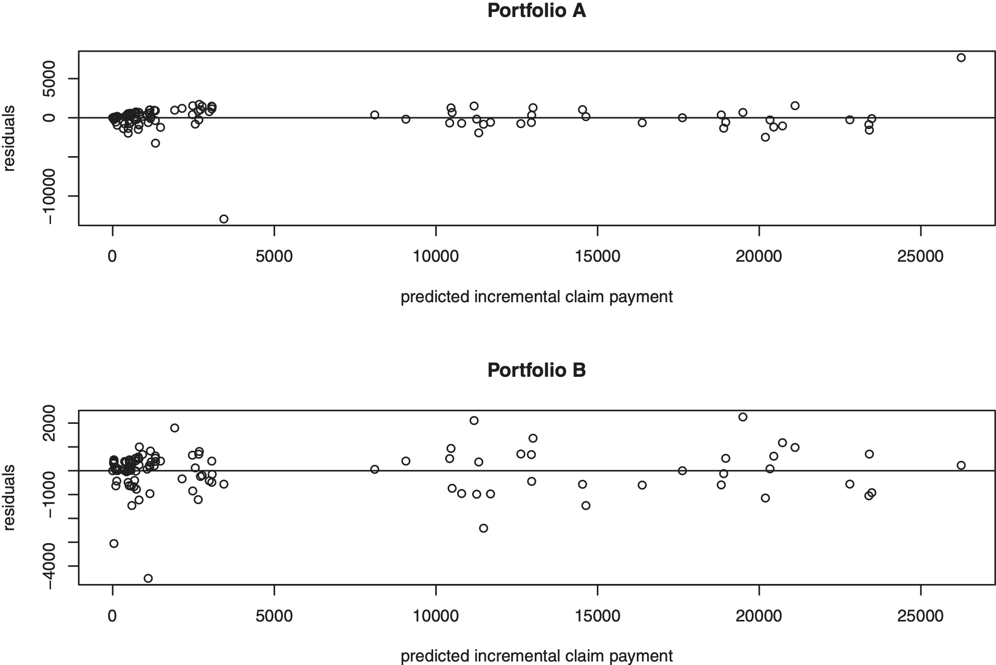
In order to choose specific $\xi$ and $\delta$, we use as a goodness-of-fit criterion the $\operatorname{SSE}(\xi, \delta)$, see (4.5), and take the parameter combination $\xi \in\{0,2\}, \delta \in\{0,2\}$ with minimum $\operatorname{SSE}(\xi, \delta)$. This method is also proposed in Chapter 11 in Wüthrich and Merz (2008) for comparing the fit to the data of different claims reserving methods. Table 4 shows that $\xi=2$ provides a much better fit than $\xi=0$ which can be explained as follows: In Model Assumptions 2.1 the incremental claim payments are of the type $\left.\mathbf{Y}_{i, j}\right|_{\Theta_i} \sim \pmb{\mu}\left(\Theta_i\right)+\varepsilon_{i, j}$ with $E\left[\varepsilon_{i, j} \mid \Theta_i\right]$ $=0$ and $\operatorname{Var}\left(\varepsilon_{i, j} \mid \Theta_i\right)=\mathbf{D}\left(\mathbf{w}_{i, j, \xi, \delta}\right)^{-1 / 2} \cdot \Sigma\left(\Theta_i\right) \cdot \mathbf{D}\left(\mathbf{w}_{i, j, \xi, \delta}\right)^{-1 / 2}$. In the case of $\xi=0$ the conditional variance $\operatorname{Var}\left(\varepsilon_{i, j} \mid \Theta_i\right)$ does not depend on development year $j$ and we assume homogeneous variances of $\left(\left.\mathbf{Y}_{i, j}\right|_{\Theta_i}\right)_{0 \leq j \leq,}$, although this assumption seems quite unrealistic. Then the weights of the standardized incremental claim payments $\mathbf{Y}_{i, j}$ in the compressed data vector $\mathbf{K}_i$ in Theorem 2.2 also do not depend on the development year j . This leads to high credibility predictors for the untypical accident years (2 and 13) and small predictors for accident year 7 for $\xi=0$ (see Table 3 ) and consequently to a high $\operatorname{SSE}(0, \delta)$. The $\sqrt{\operatorname{SSE}(0, \delta)}$ decreases by about $40 \%$ if these “untypical” accident years (2, 7, and 13) are left out in the calculation of $\sqrt{\operatorname{SSE}(0, \delta)}$. Heterogeneous variances are respected in the case $\xi=2$ leading to a much better model fit (see Table 4). Figure 2 shows the predicted claim payments versus the corresponding residuals. There is no clear trend in the plot, and the data are (approximately) centered. However, there remains the problem of untypical accident years which cannot be fitted appropriately. This problem is visualized in Figure 2, where in Portfolio A and B the highest and lowest values (outliers) result from accident years 7 and 13. The $\sqrt{\operatorname{SSE}(2,0)}$ decreases by about $57 \%$ (from 19,996 to 8,512 ) if the untypical accident years (2, 7 and 13 ) are ignored.

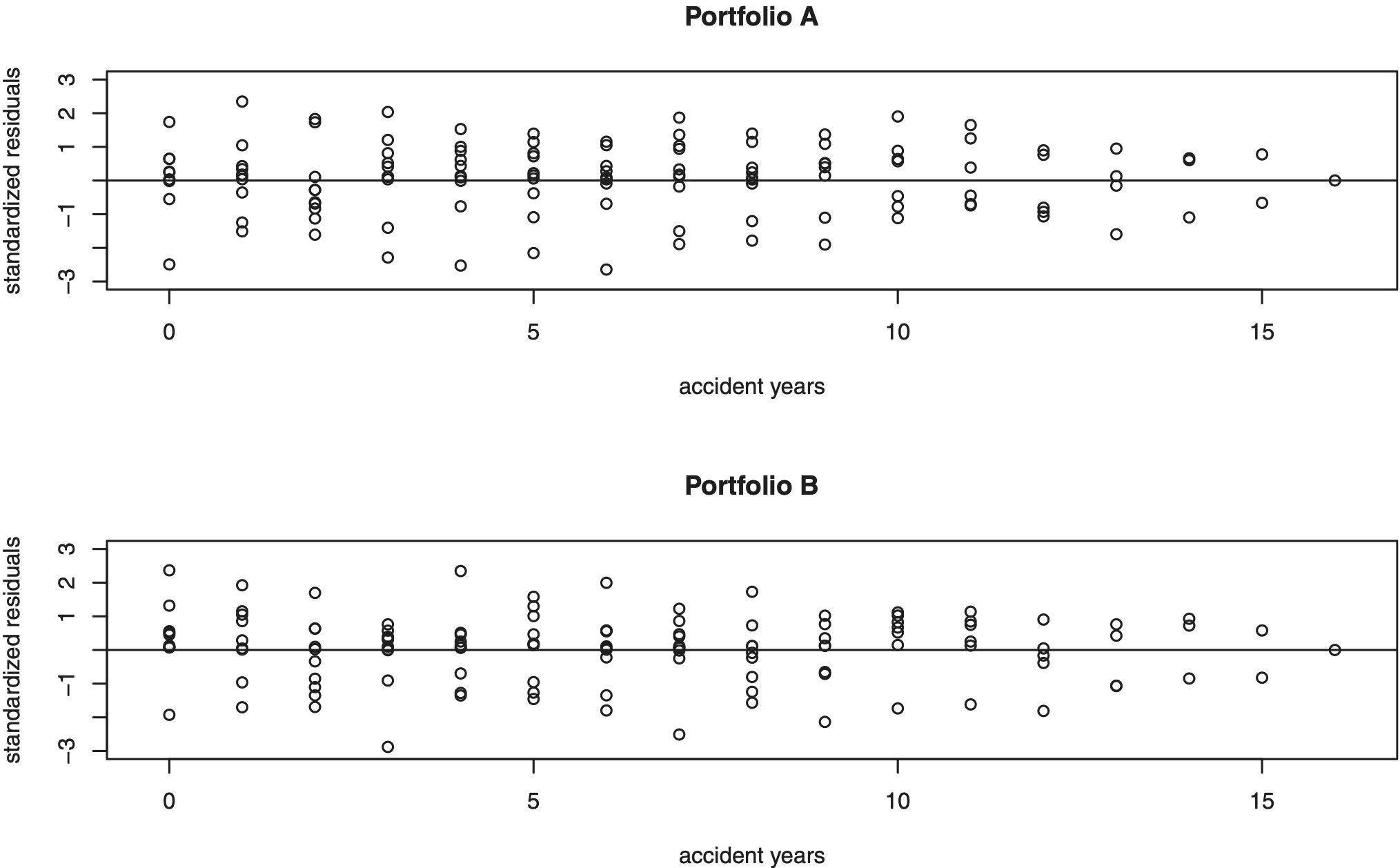
For ξ = 2 and δ = 0 we analyse the standardized residuals given by

$$\mathbf{r}_{i, j}=\mathbf{D}\left(\mu_{i}\right)^{-2} \Sigma\left(\Theta_{i}\right)^{-1}\left(\mathbf{X}_{i, j}-\mathbf{D}\left(\gamma_{j}\right) \mathbf{D}\left(\mu_{i}\right) \pmb{\mu}\left(\Theta_{i}\right)\right) . \tag{5.2}$$

These standardized residuals have, conditionally given Θ_i, zero mean and diagonal identity matrix as covariance matrix. Replacing all unknown parameters in (5.2) by their estimates leads to the empirical standardized residuals $\hat{\mathbf{r}}_{i, j}$. For Portfolio A and B, Figure 3 shows the empirical standardized residuals which are (approximately) centered and do not seem to have a trend.

We consider for the case ξ = 2 and δ = 0 the corresponding reserves 2.13 as well as the associated prediction uncertainty. Table 5 shows the estimates for the aggregated claims reserves, conditional process standard deviation, squared conditional estimation error and conditional standard error of prediction for the aggregated reserves over all accident years resulting by the multivariate Bühlmann-Straub (ξ = 2 and δ = 0), chain-ladder and additive loss reserving model. The last two columns contain the estimates of the fourth iteration for the multivariate chain-ladder and additive loss reserving model, respectively (see Merz and Wüthrich (2008), Chapter 8, for more details to the models). We obtain in the Bühlmann-Straub model higher reserves as well as a higher prediction uncertainty compared to the other two models. The difference can partly be explained by the fact that allowing for different “accident years qualities” (through ${\widehat{\mu\left(\Theta_i\right)}}^{\operatorname{cred}}$) in the multivariate Bühlmann-Straub model increases the parameter uncertainty and the process variance of the model. Tables 6 and 7 show the observed incremental claim payments in Portfolios A and B.