Advances in Common Shock Modeling

1. Introduction

The common shock model, which was introduced by Heckman and Heckman (1983), Meyers (2005, 2007), and Mildenhall (2006) and is also called contagion modeling by White (2012), is a recent approach to modeling the systematic effect of changing insurance industry and general economic environments on losses. These effects include factors specific to the insurance industry, such as the so-called underwriting cycle, as well as cycles in the overall business environment, such as economic recessions and legal changes. Often the effect of such an environmental change is to cause losses to exhibit similar behavior both within, as well as across, companies or lines of business. This behavior often takes the form of a correlation of losses within or across companies or lines of businesses. The common shock model or contagion model method attempts to capture and account for the effects of such an influential environment, which is referred to as a contagious environment. These models accomplish this by determining common factors which can be incorporated separately into both the frequency and severity distributions of effected losses. For the sake of simplicity, we use the single name contagion model to refer to the common shock model.

This paper is structured as follows: section 2 will first briefly review contagion, as applied within frequency distributions. We use the context of the negative binomial distribution to illustrate the application of frequency contagion. In section 2, we further present a new method for incorporating contagion within the binomial distribution. We remark that an incorporation of contagion within the binomial distribution, resulting in positive correlation, has not appeared in the literature, and previous authors have commented on the difficulty of achieving this. Section 3 describes how the effect of a contagious environment can be modeled within the severity component of the collective risk model. Next, section 4 describes the aggregate loss distribution under contagion modeling. Section 5 presents an elementary method that can be used to easily calibrate contagion models to empirical data. Last, section 6 provides a case study on the application of contagion modeling to general insurance losses. In particular, section 6 illustrates the application of the elementary calibration scheme from section 5 to real-world insurance data and makes clear the potential deficiency of traditional collective risk modeling as applied to aggregate annual layered losses.

2. Frequency contagion

In what follows, N_i, represents a claim count random variable (RV), where the subscript i, when present, can be interpreted as signifying the i^th line-of-business. C represents the random variable which interacts with the distribution of N_i so as to induce a contagious effect. In what follows, it will be illustrated how C often acts in a multiplicative manner on the parameters of the distribution of N_i. In this context, the contagion random variable can be viewed as representing the randomness of the parameter value, as in Bayesian analysis. In what follows, we refer to C as the contagion RV. The distribution of C can take any form, which we denote by C ∼ f(E[C], Var[C]). The only restrictions on C are:

1. C has positive support, or that all values of C are greater than 0.

2. E(C) = 1 (the expected value of the RV C is 1)

3. Var(C) = c < ∞

The quantity c also plays an important role. As c represents the variance of the contagion random variable, we also require that c ≥ 0, and refer to c as the contagion parameter.

The canonical distribution that is often used to introduce frequency contagion is the Poisson distribution. For a description of the incorporation of contagion within the Poisson distribution, the reader is referred to Meyers (2007). The literature also contains a procedure which results in a model that is equivalent to introducing contagion within the negative binomial. However, it is the belief of the authors that the traditional parameterization of the negative binomial facilitates a greater understanding of the nature of contagion modeling and also makes clear the ease of implementation. Moreover, as some statistical software is not amenable to the mean/variance parameterization of the negative binomial, some practitioners may benefit from a more explicit algorithm in this situation.

In order to explicitly illustrate how contagion can be directly introduced within a negative binomial distribution the Klugman (2012), or r, β parameterization is more useful:

$$\begin{array}{l} \operatorname{Pr}(N=n)=\binom{r+n-1}{n}\left(\frac{1}{1+\beta}\right)^{r}\left(\frac{\beta}{1+\beta}\right)^{n}\\ \text { for } n \geq 0 \text { and } \beta>0, r \in R^{+} \end{array} \tag{2.1}$$

Since the negative binomial distribution has two parameters, the contagion RV could potentially operate on the parameters r, β of the negative binomial in a multitude of ways. However, for the sake of brevity, we straightforwardly present the particular operation which is consistent with the presentation of negative binomial contagion in the literature. In a quite analogous manner to Poisson contagion, the contagion RV, C, can simply be multiplied with the parameter β, and leave the r parameter unaffected. Hence, we can describe the negative binomial distribution, under contagion, by:

$$\begin{array}{c} \qquad N \mid C \sim \operatorname{Negbin}(r, C \beta) \\ \text { with } C \sim f(E[C]=1, \operatorname{Var}[C]=c) \\ \qquad \text { where } C \in R^{+} \end{array} \tag{2.2}$$

The r and β parameterization of the negative binomial allows the incorporation of the contagion RV to be clearly illustrated. However, the characteristics of the resultant model become more clear when the negative binomial is parameterized using the mean of λ, and a dispersion parameter, γ, which is related to variance-to-mean ratio: 1 + γλ, i.e., N ∼ NegBin(λ, γ). For completeness, we note that this parameterization is related to the r and β, parameterization via N ∼ NegBin(r = 1/γ, β = γλ). Under this λ, γ parameterization, the mean λ is multiplied by the contagion RV, i.e., N|C ∼ NegBin(Cλ, γ). Notice that if C takes the constant value of 1, with probability 1, then N will be an ordinary negative binomial distribution with mean λ and variance λ(1 + γλ), or rβ and rβ(1 + β). Further, it can be seen that E(N) = E_C[E_N(N|C)] = E_C[C · λ] = E_C [C] · λ. But, since C is required to have an expected value of 1, or E[C] = 1, we have

$$E(N)=\lambda . \tag{2.3}$$

Further, since we denote Var[C] by c, it can easily be seen that

$$\operatorname{Var}(N)=\lambda(1+\lambda(c+c \gamma+\gamma)) . \tag{2.4}$$

Equation (2.4) shows that if the contagion parameter is 0, then the distribution of N reverts to the original negative binomial, whereas as c grows, the variance increases.

The introduction of contagion, across $K$ lines-ofbusiness, for which the claim count of each is modeled with a negative binomial frequency distribution, can be denoted by: $N_i \mid C \sim \operatorname{NegBin}\left(C \lambda_e, \gamma_i\right)$ for $1 \leq i \leq K$, and: $C \sim f(E[C]=1, \operatorname{Var}[C]=c)$. Next, assume that parameters of the best-fitting negative binomial have been fit to the data for each line of business. It is important to note that each $N_i$ can have different parameters, $\lambda_i$ and $\gamma_j$, or $r_i$ and $\beta_i$, after fitting to the respective data. In this case, it can be seen that the resulting correlation between $N_i$ and $N_f$ for $1 \leq i, j \leq K$ and $i \neq j$, takes the following form:

$$\rho_{N_{i}, N_{j}}=\sqrt{\frac{c \lambda_{i}}{1+\lambda_{i}\left(c+c \gamma_{i}+\gamma_{i}\right)}} \sqrt{\frac{c \lambda_{j}}{1+\lambda_{j}\left(c+c \gamma_{j}+\gamma_{j}\right)}} \tag{2.5}$$

Again, it is important to note that the correlation between N_i and N_j not only depends on the same contagion parameter, c, but also on the parameter values of each distribution; γ_i and γ_j. Hence, a unique correlation can be induced between each N_i and N_j, even though the same contagion parameter, c, is used. Equation (2.5) also shows that the level of the contagion parameter, c, impacts the correlation between N_i & N_j in a way that makes intuitive sense. Namely:

1. As $c \rightarrow 0$, which represents a weak, or absent, contagious environment, $\rho_{N_i N_j} \rightarrow 0$.

2. As $c \rightarrow \infty$, which represents a strong contagious environment, $\rho_{N_j N_j} \rightarrow \sqrt{\frac{1}{1+\gamma_1}} \sqrt{\frac{1}{1+\gamma_2}}$.

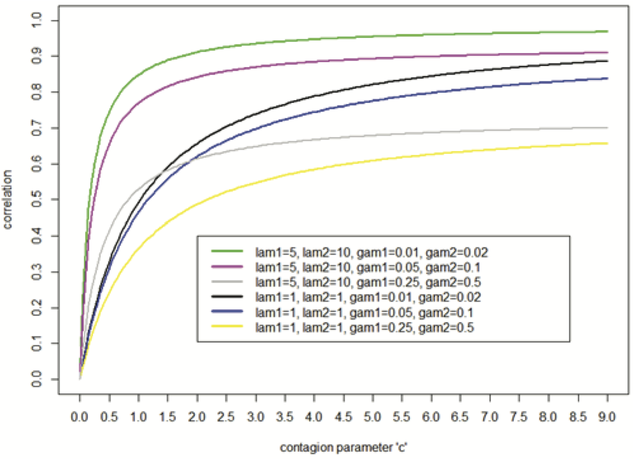
Figure 1 depicts the pair-wise correlation between $N_i$ and $N_j$ as a function of $c$, and also for different combination of the parameters, $\lambda_i \gamma_i$ and $\lambda_j \gamma_j$. It can be seen from Figure 1 that when the dispersion parameters are high, there is less correlation. There is also a trade-off between the dispersion parameters and the means, $\lambda$. Even when the dispersion parameters are relatively large, sufficiently large values of the means, $\lambda_i$, will offset the deleterious effect on the correlation caused by large dispersion parameters. Last, note that the Poisson contagion model can be achieved by setting the dispersion parameter equal to 0, and the formulas for the mean, variance, and correlation can be achieved similarly.

Figure 1.Correlation (across-lines) vs. c, and per level of negative binomial parameters

2.1. Binomial-beta contagion

Within actuarial science, claim count RV’s are often assumed to be a member of the (a, b, 0) class, which includes the Poisson, negative binomial, and binomial distributions. For information on the (a, b, 0) class, the reader is referred to Klugman (2012). Further, it has been the author’s experience that the binomial distribution is used in practice when the variance of event count data is significantly less than the corresponding mean. Moreover, we note that the existing literature on contagion modeling, including the work of Meyers (2005, 2007), considers the binomial distribution. For these reasons, we feel that the binomial distribution should not be ignored. To the authors’ knowledge, a viable method for inducing positive correlation, via contagion, between binomially distributed random variables is absent from the literature. The results of this section fill this void by presenting an original formulation for the introduction of contagion among binomially distributed random variables that results in positive correlation.

Before proceeding, the authors wish to impress upon the reader that not every association (operation) of the contagion RV with (on) the parameters of the claim count distribution will lead to a valid contagion model. In particular, in order for an association (operation) of the contagion RV to be valid, it must result in a claim count distribution with the following characteristics:

i) The mean of $N_i$ should remain unaffected.
ii) As the variance of the contagion $R V$ increases:
   a. The variance of $N$ should increase.
   b. $\rho_{N_i N_j}$ should increase.
iii) As the variance of the contagion $R V$ goes to 0 :
   a. the variance of $N$ should equal its value in the absence of contagion.
   b. $\rho_{N_i N_j}$ should go to 0 .

In addition to the preceding requirements, the following condition is often desired:

i. For a given level of the contagion parameter, the correlation between claim count RVs with large means should be stronger than the correlation between claim count RVs with small means, given that the volatilities are held constant.

The probability density for a binomial distribution with parameters n_i and p_i can be written as

$$\begin{array}{l} N \sim \operatorname{Binomial}(n, p)=\binom{n}{N} p^{N}(1-p)^{n-N}\\ \text { where } 0 \leq N \leq n \text { and } n \in R^{+}, 0<p \leq 1 \end{array} \tag{2.6}$$

First, consider a single binomial distribution. Next, assume that the best-fitting binomial distribution has been fit to the data, and results in the parameter estimates, p̂ and n̂. Now, we assume that N ∼ Binomial (n̂, p), where p is the only parameter that is considered to be random, i.e., the parameter n is evaluated at n̂. Next, consider the following prior distribution for p, where c is the contagion parameter:

$$p \sim \operatorname{Beta}\left[\alpha=\frac{1}{c}, \beta=\left(\frac{1}{c}\right) \frac{1-\hat{p}}{\hat{p}}\right] \tag{2.7}$$

Note that both p̂ and c are constants in this beta distribution. Using this distribution for p we can check that the resulting posterior predictive distribution for N has the desired properties. In particular, it can be seen that the mean is unaffected, while at the same time, larger values of c result in a larger variance. It can be easily seen that: E(N) = E_p [E_N (N|p)] = n̂ · p̂. Thus the mean of the beta-binomial mixture equals the mean of the original, best-fitting, binomial, as required. It can also be shown that the variance of the beta-binomial mixture is Var(N) = n̂p̂(1 − p̂) × (1 + n̂p̂c) × (1/(1 + p̂c)). Notice that when c → 0, Var(N) → n̂p̂ (1 − p̂), and as c → ∞ ⇒ Var(N) → n̂[n̂p̂ (1 − p̂)] > n̂p̂ (1 − p̂).

Now, let N_i be the number of claims for the i^th line of business, out of K lines of business. Again, assume that the best-fitting binomial distribution has been determined for each line. Denote the parameter estimates which specify these best-fitting binomial distributions by {n̂_i, p̂_i|1 ≤ i ≤ K}. We propose the following procedure for inducing contagion between binomial claim count RVs:

$$\begin{array}{c} N_{i} \left\lvert\, p \sim \operatorname{Bin}\left(\hat{n}_{i},\left(\frac{\hat{p}_{i}}{\hat{p}^{*}}\right) p\right) \quad\right. \text { for } 1 \leq i \leq K \\ \text { and } \quad p \sim \operatorname{Beta}\left(\alpha=\frac{1}{c}, \quad \beta=\frac{1}{c}\left(\frac{1-\hat{p}^{*}}{\hat{p}^{*}}\right)\right) \end{array} \tag{2.8}$$

where p̂* = max(p̂₁, p̂₂, . . . , p̂_n), and p̂_i is the best-fitting parameter estimate, for line i. We now illustrate that the preceding combination of claim count distributions, and the prior distribution, have the desired characteristics. First, it can easily be shown that for 1 ≤ i ≤ K, E(N_i) = E_p[E_Ni(N_i|p)] = n̂_i · p̂_i Hence, the proposed model preserves the mean of each of the marginal distributions, as required. Next, we verify that the variance of each marginal has the desired characteristics. Further, it can be shown that, for 1 ≤ i ≤ K, the variance for a single binomial RV is

$$\begin{aligned} \operatorname{Var}\left(N_{i}\right)= & \frac{\hat{n}_{i} \hat{p}_{i}\left(1-\hat{p}_{i}\right)}{1+c \hat{p}^{*}}+\frac{c \hat{p}^{*}\left[\hat{n}_{i} \hat{p}_{i}\left(1-\frac{\hat{p}_{i}}{\hat{p}^{*}}\right)\right]}{1+c \hat{p}^{*}} \\ & +\frac{c \hat{p}^{*}\left[\left(\hat{n}_{i} \hat{p}_{i}\right)^{2}\left(\frac{1}{\hat{p}^{*}}-1\right)\right]}{1+c \hat{p}^{*}} \end{aligned} \tag{2.9}$$

Though it may appear complicated, several important observations can be made from this expression. First, it can be seen that:

1. as c → 0, we have that: Var (N_i) → n̂_ip̂_i (1 − p̂_i), which is the variance of the best-fitting binomial distribution to the data from line i, in the absence of contagion.

2. Var (N_i) is an increasing function of c.

3. as c → ∞, we have

$$\operatorname{Var}\left(N_{i}\right) \rightarrow \hat{n}_{i} \hat{p}_{i}\left(1-\frac{\hat{p}_{i}}{\hat{p}^{*}}\right)+\left(\hat{n}_{i}\right)^{2}\left(\hat{p}_{i}\right)^{2}\left(\frac{1}{\hat{p}^{*}}-1\right) .$$

A little effort reveals that observation 3 illustrates that the variance behaves as required.

Next we investigate the correlation between N_i and N_j under the proposed binomial contagion model. It can be shown that the formula for the correlation between the number of claims in the i^th and j^th lines of business, where 1 ≤ i, j ≤ K, and i ≠ j, is

$$\rho_{N_{1}, N_{2}}=\frac{\hat{n}_{i} \hat{p}_{i} \hat{n}_{j} \hat{p}_{j}\left(\frac{c\left(1-\hat{p}^{*}\right)}{1+c \hat{p}^{*}}\right)}{\sigma_{i} \sigma_{j}} \tag{2.10}$$

where σ_i² is as in equation (2.9).

From Equation (2.10), several observations regarding $\rho_{N_i N_j}$ as a function of $c$, can be made. For $1 \leq i$, $j \leq K$ and $i \neq j$, we have:

1. as $c \rightarrow 0$, we have $\rho_{N_1 N_2} \rightarrow 0$.
2. $\rho_{N_1 \cdot N_2}$ in an increasing function of $c$.
3. as $c \rightarrow \infty$, it can be shown that:

$$\rho_{N_{i}, N_{j}} \rightarrow \frac{1}{\sqrt{\left(1+\frac{\left(\hat{p}^{*}-\hat{p}_{i}\right)}{\hat{n}_{i} \hat{p}_{i}\left(1-\hat{p}^{*}\right)}\right)\left(1+\frac{\left(\hat{p}^{*}-\hat{p}_{j}\right)}{\hat{n}_{j} \hat{p}_{j}\left(1-\hat{p}^{*}\right)}\right)}}$$

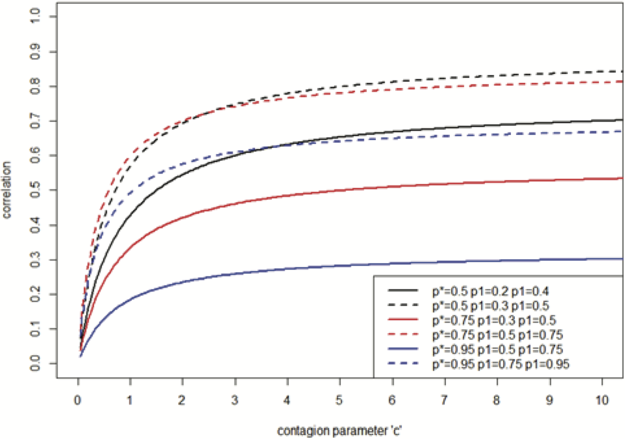
Figure 2 illustrates the pair-wise correlation, under binomial contagion, for various levels of p̂*, p̂₁, and p̂₂. n̂ = 5 is used throughout.

Figure 2.Correlation vs. c, per level of binomial parameters, and p*

Note that, as for the Poisson and negative binomial models, different levels of correlation between different pairs of RV’s can be achieved, despite the use of a single contagion parameter. This is so, since the pair-wise correlations depend on the parameter values of the best fitting binomial distributions n̂_i, p̂_i, and n̂_j, p̂_j, for each line, as well as on c. From Figure 2, it can also be seen that the correlation is higher between lines for which both p̂_i and p̂_j are relatively large, and hence have a relatively large number of counts, on average (n̂_i constant). Also note, from the pairs of black, red, and blue lines, that for the particular levels of p̂_j in this example, a higher value of p̂* results in lower correlations.

3. Severity contagion

In traditional severity modeling, the assumption that all severities are independent is made, largely, to make both the mathematics and implementation easier. This is the case, despite the fact that patterns in loss severities, over time, have been documented by practitioners. One such example is the so-called property and casualty insurance underwriting cycle. Further, some believe that loss trends are a significant driver of premium rates. Moreover, it is reasonable to assume that loss trends are, in turn, driven by a set of endogenous factors, such as changes in underwriting standards and policy terms, and exogenous factors, which include the legal and regulatory environment. In the traditional contagion modeling framework, the goal is to partition a company’s portfolio into a set of mutually exclusive and exhaustive subsets, where the combined effect of these drivers of loss trend is relatively constant within each subset and varies more markedly across subsets. Moreover, traditional contagion modeling attempts to capture the combined effect of all drivers, within any such subset, with only a small set of contagion parameters. Hence, the distinct levels of the contagion parameters represent what’s referred to as a contagious environment. We remark that some may consider the goal of achieving such a parsimonious model to be quixotic; however, one should keep in mind the alternative. It is well known that calibrating correlation matrices is notoriously difficult, especially for a large number of variables.

Another well-known characteristic of traditional contagion modeling is its ability to represent parameter uncertainty within simulation models. A byproduct of this inclusion of parameter uncertainty is an inflation in the variance of the marginal loss distributions. In this section we propose an alternative to traditional contagion modeling that can be viewed as an option for more conservative (re)insurers, who may be uneasy with the increase in variance associated with the traditional model, or (re)insurers who place a large amount of significance in their data. As with traditional contagion modeling, the proposed form of severity contagion induces correlation; however, the proposed method has the benefit of minimizing the distortion of the variance of the marginal distributions. We represent the observed loss severity of the $k^{\text {th }}$ line of business by $X_k$, and denote that $X_k$ follows a distribution with mean $\mu_k$ and, variance $\sigma_{x_k}^2$, by $X_k \sim \operatorname{Dist}_k\left(E\left[X_k\right]=\mu_k, \operatorname{Var}\left[X_k\right]=\sigma_{x_k}^2\right)$. The proposed method accomplishes this by supposing that the size of each loss can be decomposed into two components. The first component is governed solely by a theoretical, unadulterated, underlying, loss distribution, and the second component represents the impact of the contagious environment on the size of loss. The former can be loosely thought of as an idiosyncratic component and the latter a systematic component. Consider the losses from the $k^{\text {th }}$ line of business. We denote the idiosyncratic component by the $R V, Z_k$, and the systematic component by the $R V, \beta$. Specifically, we assume that $X_k$ can be decomposed into the product of two $R V^{\prime} s: \beta Z_k$, where $\beta$ is the severity contagion $R V$, and $Z_k$, the underlying loss $R V$. Analogous to frequency contagion, we use $b$ to represent the contagion parameter. The motivation for this decomposition of $X_k$ arises mainly from the desire to separate the portion of the variation of $X_k$ that is solely due to the random claims generation process from the portion of the variance that is due to the contagious environment. Further, it should be noted that the proposed decomposition of the observed losses requires the elucidation of information from the data, over and above that required by existing severity contagion models. As is usually the case, there is a cost associated with this additional precision. In this case, the additional cost comes in the form of increased complexity in calibrating the model. Specifically, instead of the need to only determine the best-fitting contagion parameter, b (to be defined shortly), it is also necessary to determine the RV, Z_k, which best describes the pure loss process. Before proceeding, the authors wish to point out that they are not implying that the variance inflation that is associated with traditional contagion modeling is a shortcoming of the traditional severity contagion model.

As with the traditional version of severity contagion, the only requirements on the RV β are that its distribution has positive support and that its mean be 1. Aside from this, β can have any distributional form, which we denote by β ∼ f(E(β), Var(β)). Also, since the observed losses are modeled by the product of RV’s, i.e., β · Z_k, or using slightly simpler notation; βZ_k, additional requirements must be imposed, namely that:

1. β be independent of Z_k, and

2. E(Z_k) = E(X_k).

In summary, the proposed severity contagion method models the size of observed losses by $\beta Z_k$ where $Z_k \sim$ $\operatorname{Dist}_k\left(E\left[Z_k\right]=\mu_k, \operatorname{Var}\left[Z_k\right]=\sigma_{z_k}^2\right)$ and $\beta \sim f(E(\beta)=1$, $\operatorname{Var}(\beta)=b)$, with $b \geq 0$, and, further, such that $E\left(Z_k\right)=$ $\mu_{z k}=\mu_k=E\left(X_k\right)$ and $\operatorname{Var}\left(Z_k\right)=\sigma_{z_k}^2 \leq \sigma_{x_k}^2=\operatorname{Var}\left(X_k\right)$. Further, since the variance of $\beta$ represents only a small fraction of the overall variance of $X_k$, the assumption that $Z_k$ is a member of the same family of distributions as $X_k$ should be, at most, venial.

We note that the proceeding model formulation has the desired characteristics, namely, that the mean of $X_k$ is preserved by the proposed model, since $E\left[\beta Z_k\right]=$ $E[\beta] E\left[Z_k\right]=\mu_k$ and that the variance has the following form:

$$\operatorname{Var}\left[\beta Z_{k}\right]=\sigma_{z_{k}}^{2}+b\left(\mu_{k}^{2}+\sigma_{z_{k}}^{2}\right) . \tag{3.1}$$

We now consider the reasonableness of the proposed severity contagion method. If the overall severity model accurately represents the impact of a contagious environment on the pure loss generation process, and a calibration scheme is able to effectively isolate the contribution of $\beta$ to the variation of the data, then, at least theoretically, it should be possible to determine parameters, $\mu_k, \sigma_{2 k}^2$, and $b$, such that: $\operatorname{Var}\left(X_k\right) \approx \operatorname{Var}\left[\beta Z_k\right]$. This makes sense, since:

1. In the absence of a contagious environment, it should be inferred that $\sigma_{z_k}^2 \approx \sigma_{x_k}^2$, and hence $\sigma_{x_k}^2=$ $\operatorname{Var}\left(X_k\right) \approx \operatorname{Var}\left[\beta Z_k\right]=\sigma_{z_k}^2+b\left(\mu_k^2+\sigma_{z_k}^2\right)$, which implies that $b=0$, or that $\operatorname{Var}[\beta]$ is small.

2. Alternatively, in the presence of a strong contagious environment, it should be inferred that $\sigma_{z_k}^2 \ll \sigma_{x_k}^2$, which, by the same argument, implies that $\operatorname{Var}[\beta] \gg 0$, or in other words that $b \gg 0$.

Conversely, under the same assumption that $\operatorname{Var}\left(X_k\right)=\operatorname{Var}\left[\beta Z_k\right]$, we have that:

1. $b=0$ implies that $\sigma_{z_k}^2=\operatorname{Var}\left[\beta Z_k\right]=\operatorname{Var}\left(X_k\right)=\sigma_{x_k}^2$, which implies a weak contagious environment, and

2. $b \gg 0$ implies that $\sigma_{x_k}^2=\operatorname{Var}\left(X_k\right) \approx \operatorname{Var}\left[\beta Z_k\right]=$ $\sigma_{i_k}^2+b\left(\mu_k^2+\sigma_{i_k}^2\right) \gg \sigma_{z_k}^2$, which implies a strong contagious environment.

To illustrate the difference between the traditional and proposed severity contagion models, by fitting $X_k$ to the data, and then multiplying by $\beta$, as in the traditional contagion model, we have that $\operatorname{Var}\left[\beta X_k\right]=$ $\sigma_{x_k}^2+b\left(\mu_k^2+\sigma_{x_k}^2\right)>\sigma_{x_k}^2 \approx \operatorname{Var}[$ data $]$. As mentioned previously, this distortion of the variance would likely not be of concern to (re)insurers who have limited data, or ascribe less credibility to their data, or who may even believe that the observed data does not accurately represent the true, theoretical, variance.

We now investigate the proposed model’s ability to induce correlation between two or more loss $R V$ 's. Let Dist $\mathstrut_k$ denote the best-fitting distribution to the data from the $k^{\text {th }}$ line of business, and Dist $t_j$ denotes the best-fitting distribution to the data from the $j^{\text {h }}$ line of business. Further, assume that $X_k$ and $X_j$ can be, sufficiently, modeled as the product of $R V$, which we denote by $X_k=$ $\beta Z_k$ and $X_j \approx \beta Z_j$, where $\beta$ is independent of $Z_k$ and $Z_j$, and $Z_k$ is independent of $Z_j$. Further, assume that the parameters of $Z_k, Z_j$, and $\beta$ are $\sigma_{z k}^2, \sigma_{z j}^2$, and $b$. Then, it can be seen that the covariance between $\beta Z_k$, and $\beta Z_j$ is: $\operatorname{Cov}\left(\beta Z_k, \beta Z_j\right)=\mu_k \mu_j b$.

Next, this result can be used to show that the correlation between $\beta Z_k$, and $\beta Z_j$, is:

$$\rho_{\beta Z_{k}, \beta Z_{j}}=\frac{b}{\sqrt{\left[b+(1+b) C V_{Z_{k}}^{2}\right]\left[b+(1+b) C V_{Z_{j}}^{2}\right]}} \tag{3.2}$$

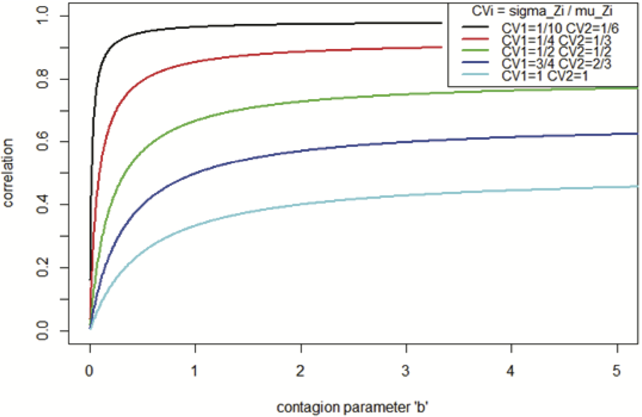
Figure 3 illustrates the correlation induced between two lines of business as a function of the contagion parameter, b, and the CV’s of Z_k and Z_j: CV²_zk = σ²_zk/μ²_k, and CV²_zj = σ²_zj/μ²_j). Further, it can be seen that when the variation in loss size is small, the correlation which can be achieved is higher, which is consistent with intuition.

Figure 3.Correlation vs. b, and per the CV’s of lines j and k

4. Aggregate loss contagion model

In this section, we describe how both frequency and severity contagion can be combined within the collective risk model (CRM). Let $N_i^*$ represent frequency distribution for line $i$, under contagion, i.e., $N_i^* \mid C \sim$ Poisson $(C \cdot \lambda)$ with $C \sim f(E[C]=1, \operatorname{Var}[C]=c)$. Further, assume that the best-fitting severity distribution to line $i$ is $\operatorname{Dist}_{x_i}\left(\mu, \sigma_{x_i}^2\right)$, where $\mu$, and $\sigma_{X_i}^2$ represent the mean and variance of the distribution of $X_i$, and that it is possible to determine parameters $\sigma_{Z_i}^2$ and $b$, such that $X_i=\beta Z_i$, where $\beta$ is independent of $Z_i$, as in Section 3. Then, we can simply replace $N_i$ with $N_i^*$, and $X_i$ with $\beta Z_i$ within the traditional CRM, to arrive at the aggregate loss distribution under both frequency and severity contagion, which we denote by $S^*$ :

$$S_{i}^{*}=\sum_{k=1}^{N_{i}^{*}} \beta Z_{i_{k}} \tag{4.1}$$

Despite the addition of contagion, it can be shown that the mean of the CRM remains unchanged, i.e., E[S*] = λ · μ. Also, it can be shown that the variance of the aggregate loss, under both frequency and severity contagion, is

$$\begin{array}{l} \operatorname{Var}\left[S^{*}\right]=\operatorname{Var}\left[Z_{i}\right] E\left(N^{*}\right)+\left(E\left[Z_{i}\right]\right)^{2} \operatorname{Var}\left(N^{*}\right) \\ \quad+b \cdot\left\{\operatorname{Var}\left[Z_{i}\right] E\left(N^{*}\right)+\left(E\left[Z_{i}\right]\right)^{2} E\left(N^{* 2}\right)\right\} . \end{array} \tag{4.2}$$

We remark that this formula works for any frequency and severity distributions. One can simply substitute in the formulas for the mean and variance of the frequency, under contagion, which we denote by E(N*) and Var(N*). E(N*) and Var(N*) will depend on the type of frequency distribution used but will not depend on the distributional form of the contagion RVs; C, or β. Hence, Equation (4.2) is a fully general formula.

We now investigate the correlation between the aggregate losses from two lines, S^*_k and S^*_j, where k ≠ j. It can be shown that the correlation between S^*_k and S^*_j, for k ≠ j, is

$$\begin{aligned} \rho_{s_{k}^{*} s_{j}^{*}}= & \frac{\lambda_{k} \mu_{k} \lambda_{j} \mu_{j}}{\sqrt{\left(\sum_{k}+b \cdot\left[\sum_{k}+\left(\mu_{k} \lambda_{k}\right)^{2}\right]\right)}} \\ & \times \frac{(c b+b+c)}{\sqrt{\left(\sum_{j}+b \cdot\left[\sum_{j}+\left(\mu_{j} \lambda_{j}\right)^{2}\right]\right)}} \end{aligned} \tag{4.3}$$

Note that ∑_i = Var[Z_i]E(N*) + (E[Z_i])² Var(N*) is the aggregate loss variance for contaged frequency and un-contaged severity.

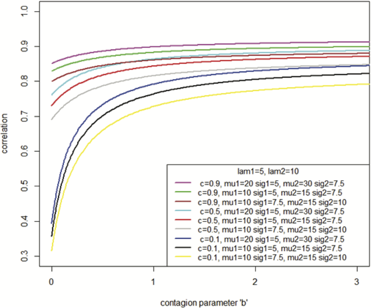
Figure 4 illustrates the correlation induced between the aggregate losses of two lines of business as a function of the contagion parameter, b. Each of the nine graphs uses 5 and 10 for the means of the two frequency distributions, i.e., λ₁ = 5, and λ₂ = 10, and corresponds to one of three levels of the frequency contagion parameter, c = 0.1, 0.5, and 0.8. It can be seen that higher levels of the frequency and severity contagion parameters c and b result in higher correlation between the lines. Also, higher levels of μ_j result in higher correlation. Conversely, higher levels of σ_j result in lower correlation. Or, stated another way, the greater the uncertainty in the loss sizes of each line, the more tenuous the relationship between the loss sizes, and hence the lower the correlation.

Figure 4.Correlation of aggregate losses vs. b, per level of c, and the mean and SD of the severity distributions

Moreover, in the special case where the claim frequency for both line j and k, are Poisson, it can be shown that the correlation between S^*_k and S^*_j, for k ≠ j, is

$$\begin{aligned} \rho_{S_{k}^{*}, s_{j}^{*}}^{*}= & \frac{1}{\sqrt{\left[(1+b) C V_{S_{k}}^{2}+[b c+b+c]\right]}} \\ & \times \frac{(c b+b+c)}{\sqrt{\left[(1+b) C V_{S_{j}}^{2}+[b c+b+c]\right]}} \end{aligned} \tag{4.4}$$

5. Implementation and calibration

In this section we illustrate one out of many potential methods for calibrating contagion models to empirical data. The motivation for illustrating this particular calibration procedure is three-fold. First, it is a very simple, and practical, way to calibrate contagion models to per-claim empirical data. Further, there appears to be a dearth of literature that describes, in detail, practical approaches to calibrate contagion models to such per-claim empirical data. In fact, to the authors’ knowledge, this paper represents the first attempt to do so. Second, the authors wish to illustrate that the proposed severity contagion model, specifically, can be calibrated with this simple technique. Third, while the authors recognize that advanced statistical techniques, such as the EM algorithm, GLMs or GLMMs, should ideally be used to calibrate the proposed severity contagion model, where Var[data] ≈ Var[βX_k], it is very unlikely that the practicing actuary will have sufficient data at their disposal to attain statistically significant results from these methods.

We first investigate the calibration for a single line of business. The procedure employed will, no doubt, depend on the purpose of the analysis as well as the expert opinion of the practitioner. There are three main steps for calibration of contagion models for aggregate losses:

1. Model fitting—determination of the best-fitting distributions for the frequency and severity, based on the empirical data.

2. Calibration of the frequency contagion model, based on the empirical claim count data.

3. Calibration of both the pure, underlying, loss process, Z_i, and also the contagion RV β.

Step 2 is accomplished by exploiting the corresponding formula for the variance of the claim count RV under contagion. For example, when claim counts are modeled with a Poisson distribution, with mean λ, we have that Var(N) = λ(1 + c · λ). As Var(N) can be estimated from the observed annual claim count data, the only unknown quantity is the frequency contagion parameter c. Hence, the above equation can be rewritten to solve for c:

$$c=\frac{\operatorname{Var}(N)}{\lambda^{2}}-\frac{1}{\lambda} \tag{5.1}$$

Step 3 calibrates the proposed severity calibration method. As mentioned in section 3, given the inevitable uncertainty surrounding the true underlying loss process, as well as the presumed relatively small variance of β, in most circumstances, there is no harm in assuming that the RV Z_k follows the same distributional form as the best-fitting distribution to X_k. Hence, the determination of the distribution of Z_k only requires the determination of its variance, σ²_z. Again, if sufficient data were available, it would be preferred to use advanced statistical procedures, such as the EM algorithm, GLMs, or GLMMs. However, as this is usually not the case, we describe a simple, straightforward severity calibration method. To accomplish step 3 we perform the following steps:

1. Determine b.

2. Use this b to determine σ²_z.

3. Determine the parameters of the severity distribution (Pareto, in this case), which correspond to this σ²_z, and use this severity distribution within the simulation.

Using Equations (3.1) and (4.2) if claim frequency is assumed to follow a Poisson distribution with parameter λ, then it can be shown that

$$b=\frac{\operatorname{Var}\left[S^{*}\right]-\lambda \cdot \operatorname{Var}[\beta Z]-\lambda \mu_{z}^{2}-\lambda^{2} \mu_{z}^{2} c}{\lambda^{2} \mu_{z}^{2}(1+c)} \tag{5.2}$$

In Equation (5.2), $\operatorname{Var}\left[S^*\right]$ is the variance of the empirical aggregate losses, and $\mu_Z\left(=\mu_x\right)$ and $\operatorname{Var}[\beta Z] \approx$ $\operatorname{Var}[X]$ can be estimated using the mean and the variation, respectively, of the per-claim loss data. Recalling that $c$ has already been estimated, at this stage, all remaining quantities to the right of the equals sign in Equation (5.2) can be estimated from the empirical data. Note that Equation (5.2) only applies to the specific case of a Poisson frequency. However, when contagion is introduced within a negative binomial frequency the corresponding formula can be shown to be

$$\begin{aligned} b= & \frac{\operatorname{Var}\left[S^{*}\right]-\lambda \cdot \operatorname{Var}[\beta Z]}{\lambda^{2} \mu_{z}^{2}(1+c+\gamma+c \gamma)} \\ & -\frac{\lambda \mu_{z}^{2}+\lambda^{2} \mu_{z}^{2} c+\lambda^{2} \mu_{z}^{2} \gamma(1+c)}{\lambda^{2} \mu_{z}^{2}(1+c+\gamma+c \gamma)} \end{aligned} \tag{5.3}$$

Once b has been determined, the variance of the pure underlying loss RV, Z, can be solved for using Equation (3.1):

$$\sigma_{z}^{2}=\frac{\operatorname{Var}[\beta Z]-b \mu_{z}^{2}}{1+b} \approx \frac{\operatorname{Var}[X]-b \mu_{z}^{2}}{1+b} \tag{5.4}$$

Finally, the aggregate annual losses, under both frequency and severity contagion, are

$$S^{*}=\sum_{i=1}^{N^{*}} \beta Z_{i} \tag{5.5}$$

where

$$\begin{array}{l} N^{*} \mid C \sim \operatorname{Dist}_{N}(C \cdot \lambda) \quad \text { with }\\ C \sim f(E[C]=1, \operatorname{Var}[C]=c) \end{array} \tag{5.6}$$

and

$$\left\{\begin{array}{c} Z_{i} \sim \operatorname{Dist}_{X}\left(E\left[Z_{i}\right]=\mu_{z}=\mu_{x}, \operatorname{Var}\left[Z_{i}\right]=\sigma_{z}^{2}\right), \\ Z_{i} \text { and } Z_{j} \text { are independent of each other for } i \neq j \\ \beta \sim f(E(\beta)=1, \operatorname{Var}(\beta)=b) \end{array}\right. \tag{5.7}$$

As indicated above, this is just one method for calibrating contagion models. This particular method is informed by the desire to produce aggregate annual loss simulations with variation close to the variation of the empirical annual aggregate losses. Armed with an understanding of the proposed calibration method for a single line of business, various calibration procedures can be employed to extend the calibration to two or more lines of business. We leave the choice of the specific calibration procedure to the practitioner.

6. Case study: Natural peril data

In this case study, we consider only a single line-of-business. Further, we compare the ability of two models to reproduce key characteristics of a sample of historical data. The key characteristic of the simulated values that we focus our attention on is the coefficient of variation (CV). The two models under consideration are:

1. The traditional CRM, and

2. The CRM under contagion.

Both models 1 and 2 will be calibrated to the actual loss data. In particular, the data will be used to determine both the distributional choices (frequency and severity), as well as parameter values of each. In other words, we allow the data to dictate the calibration both models.

Next we turn our attention to the data used in this case study. The data is actual loss data consisting of 670 property claims from severe convective storms between years 2003 and 2012, inclusive. The data is on an occurrence basis and is in units of $1,000. Due to the proprietary nature of the data, only approximate values of the corresponding aggregate annual losses are shown in Table 1. The approximate nature of these values should be kept in mind, should the reader attempt to verify the results presented in this section using values from Table 1.

We now proceed to the analysis of the data. Since the variance of the annual claim counts Var(N) (≅ 600) is significantly greater than the mean E(N) (≅ 70), we use a negative binomial distribution for the frequency distribution, both within the CRM and the CRM under contagion. Specifically, based on the annual aggregate claim data, we use

$$\begin{array}{c} p=\operatorname{prob} \text { success }=\frac{E[X]}{\operatorname{Var}[X]} \cong 0.1, \\ r=\frac{E[X]^{2}}{\operatorname{Var}[X]-E[X]}=8.25 \end{array}$$

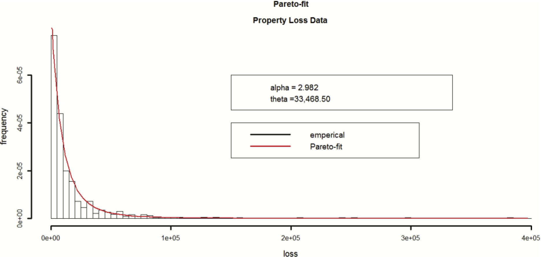
We now turn our attention to calibrating the severity component of the contagion model. Using maximum likelihood (MLE) methods, the best-fitting distribution to the observed per-claim severity is a Pareto distribution. Further, the MLE-based parameters of the best-fitting Pareto are α_MLE = 2.982, θ_MLE = 33,468.

The fit of the Pareto distribution to the observed empirical data is illustrated in Figure 5.

Figure 5.Comparison of fitted and empirical densities of the severity data

From Figure 5, it can readily be seen that the Pareto provides a good fit to the data. Although the MLE estimates of the parameters can be used within the simulation, we opt to use the method-of-moment estimates, (α_MoM, θ_MoM) = (2.876, 33,470), out of a desire to eliminate any bias in the final comparison between the two models. Also, out of a desire to be transparent, Table 2 summarizes both the method of moments and MLE parameterization of the Pareto distribution.

Again, to be fair, the final calibration of the first model (traditional CRM) uses NegBin(p = 0.11, r = 8.25) and Pareto(α = 2.87, θ = 33,470). We now calibrate the severity component of the second model (CRM under contagion). First, we use Equation (5.2) to determine the severity contagion parameter.

$$b=\frac{\operatorname{Var}\left[S^{*}\right]-\lambda \cdot \operatorname{Var}[\beta Z]-\lambda \mu_{z}^{2}-\lambda^{2} \mu_{z}^{2} c}{\lambda^{2} \mu_{z}^{2}(1+c)} \approx 0.13 .$$

The inputs that we used for Equation (5.2) are:

• The mean of the Poisson frequency distribution (l = 70).

• The modeled mean of the per-claim severity distribution (μ_z = 17,842).

• The modeled variance of the per-claim severity (Var[βZ] = σ²_x = 32,329²).

• The empirical variance of the annual aggregate losses (AAL): (Var[S*] = 697,245²).

Note that Equation (5.2) is used, since the negative binomial distribution (without contagion) is equivalent to the Poisson distribution, under contagion. As illustrated in Meyers (2007), c equals the dispersion parameter of the negative binomial: c = (Var[X] − E[X])/(E[X])∧2 = 0.12.

However, severity calibration for the second model is not complete. Recall that under the proposed severity contagion model, the true, underlying, loss process variance is elicited from the observed variation. As explained in Section 5, a simple, straightforward approach is to use Equation (5.4), together with the value of b:

$$\sigma_{z}^{2}=\frac{\operatorname{Var}[\beta Z]-b \mu_{Z}^{2}}{1+b}=29,634^{2} .$$

If a statistical software package is used that does not allow the parameterization of the Pareto using the mean and variance, the parameter values can be solved for in terms of the mean and variance. For the Pareto distribution, the corresponding formulas are

$$\begin{array}{l} \alpha=\frac{2 \operatorname{Var}[Z]}{\operatorname{Var}[Z]-E[Z]^{2}}, \\ \theta=E[Z]\left(\frac{\operatorname{Var}[Z]+E[Z]^{2}}{\operatorname{Var}[Z]-E[Z]^{2}}\right) \end{array} \tag{6.1}$$

The resulting parameters are α_Z = 3.137 and θ_Z = 38,133. At this point the calibration of the severity component of model 2 (CRM under contagion) is complete, and we can begin the simulations that are at the core of this study.

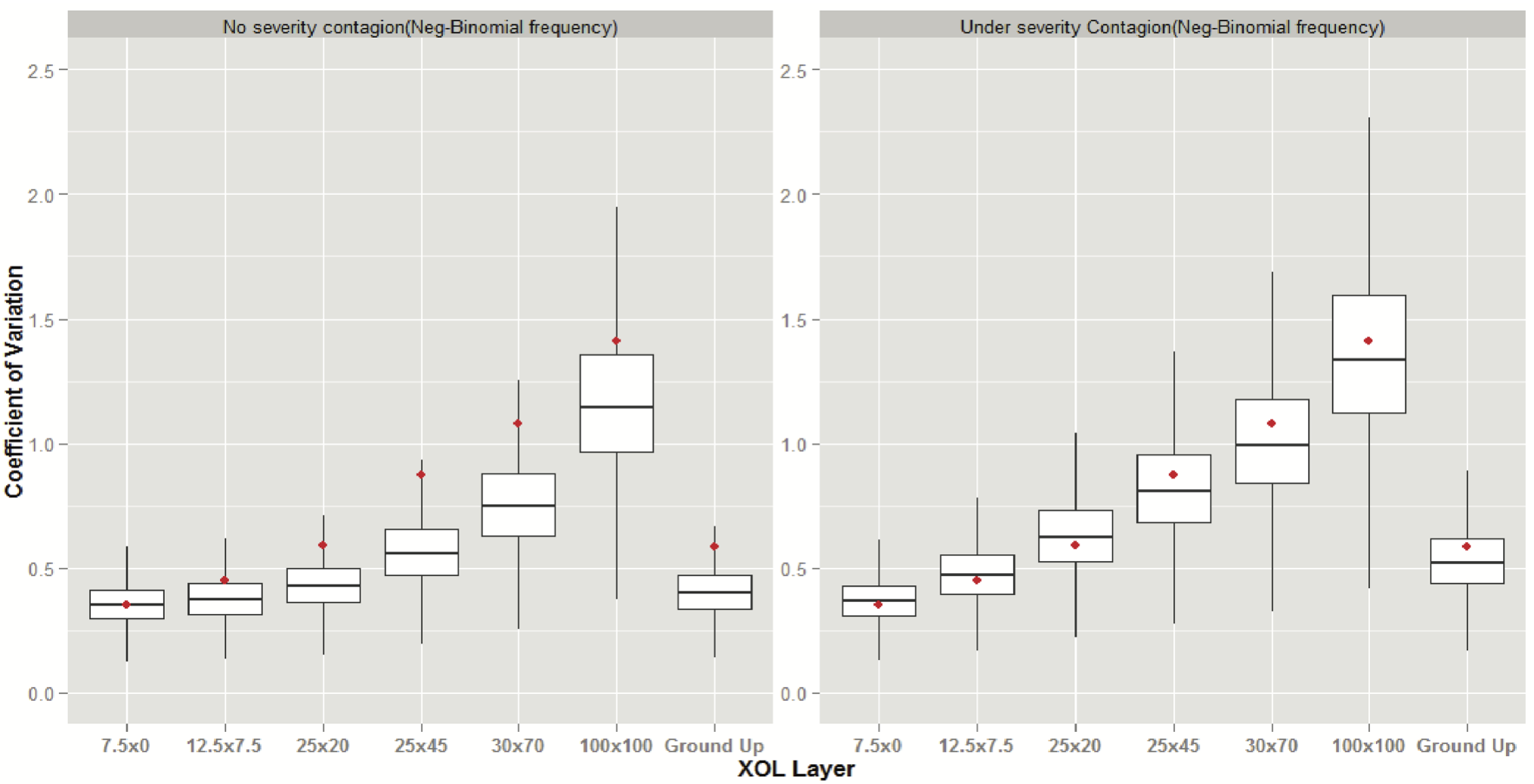
First, we define the layers of loss, which will be used for all simulations in the case study: 0 – 7.5M, 7.5M – 20M, 20M – 45M, 45M – 70M, 70M – 100M, and 100M – 200M.

The simulation study is accomplished by repeatedly simulating 10 years of aggregate annual layered losses (AALL) and then calculating the corresponding coefficient-of-variation (CV) of each set of 10-year AALLs. We do this using both AALL estimates from the traditional CRM and estimates from the CRM under contagion. This process is repeated until 100,000 10-year CV estimates are obtained under the traditional CRM and also under the CRM under contagion. Next, box-plots of both sets of CV’s are displayed, along with the empirical AALLs (red dots). For reference, the final parameterization of both models is displayed in Table 3. A summary of the simulation procedure is as follows:

1. For each iteration of the simulation, generate 10 years of Aggregate Annual Losses under both:

   • The traditional CRM

   • The CRM under contagion

2. For each of the predefined layers, calculate the annual aggregate layered loss.

3. For each set of 10 AALLs, calculate the CV.

4. Repeat 100,000 times.

   • At this point, we have 100,000 10-year CV estimates for each layer.

5. For each layer, create a box-plot using the 100,000 10-year CVs (10th, 25th, 50th, 75th, and 90th percentiles).

Note that different severity parameters were used for the traditional CRM and the CRM under contagion. Again, this is not an accident, for recall that under the proposed severity contagion method, the parameterized severity distribution represents the true underlying loss process, Z, whereas under the traditional CRM, it is the observed severity, X, that is parameterized.

Recall that the empirical CV’s of the aggregate annual layered losses are shown in red. Also, the box-plot of the ground-up losses are shown on the far right column of each graph.

Figure 6 illustrates that model 2 (CRM under contagion) produces simulated AALLs for which the 10-year CVs are more consistent with the observed CVs of the empirical AALLs. Also, recall that both the frequency and severity distributions of both models were calibrated to the observed data. Moreover, note that incorporation of a single contagion parameter allowed for the simulation of 10-year CVs that are more consistent with the observed CVs for all layers as well as for the ground-up losses.

Figure 6.Box plots of the coefficient-of-variation(CVs) of aggregate annual layered losses: Both with severity contagion (right), and without contagion (left)

7. Conclusion

Within the insurance industry, the ability to accurately capture variation instead of just the mean has grown over the past several decades. In particular, risk measures such as Value-at-Risk (VaR) and Conditional Tail Expectation (CTE) or Tail-VaR (TVaR) were constructed to capture such distributional qualities. The use of contagion within the traditional CRM will allow actuaries and risk professionals to reap the benefits of these modern risk measures.

In this paper we have investigated the contagion modeling paradigm, as introduced by Meyers (2007). First, we have elucidated, analytically, the impact of this modeling paradigm, in particular the induced correlation. Further, this has been done for frequency, severity, and aggregate contagion models under all of the common frequency and severity distributions. Second, we have developed a workable version of contagion modeling under the binomial distribution that produces positive correlation. Third, we have proposed a form of severity contagion for (re)insurers, with highly credible data, who wish to avoid the variance inflation associated with traditional contagion modeling. We have also described a procedure to calibrate aggregate contagion models, under the proposed severity contagion, based on per-claim empirical data. Last, we have demonstrated the efficacy and ease of use of the proposed calibration procedures using a real-world dataset from the insurance industry. This case study illustrates the well-known limitations of traditional collective risk modeling and provides evidence that contagion modeling provides a systematic way to correct for the inherent limitations of traditional collective risk modeling. It is our hope that this work will help establish contagion modeling, both among academics and practitioners, and also motivate additional research on contagion modeling, as well as on other ways to improve traditional collective risk modeling.

Acknowledgments

The authors wish to recognize the contribution to the following parties:

Benedict M. Escoto, PhD, FCAS, Aon Benfield Chicago, Illinois, for being willing to share his knowledge on contagion modeling and supporting calibration.

Steven B. White, FCAS & Chief Actuary, Guy Carpenter, LLC, for sharing his contagious enthusiasm for contagion modeling with us.

Stuart Sadwin, FCAS, MAAA, SVP, and Chief Corporate Actuary, TMNA Services, LLC, for his invaluable support on the model calibration.