Minimum Bias, Generalized Linear Models, and Credibility in the Context of Predictive Modeling

undefined

1. Introduction

As predictive models that relate losses (pure premiums, claim counts, average severity, etc.) to explanatory risk characteristics become ever more commonplace, some of the practical problems that frequently emerge include the following:

• Models often use complex techniques that are effectively “black boxes” without a lucid conceptual basis.

• Models may require very detailed parametric or distributional assumptions. Invalid assumptions may result in biased parameters.

• A highly frequentist approach, usually involving maximum likelihood estimation (MLE), can lead to overfitting sparsely populated data bins.

Some long-standing methods can be combined to overcome these problems:

• Minimum bias iterative fitting of parameters is simple, long-standing in practice, and nonparametric in specification.

• Credibility methods are similarly simple and long-standing; moreover, credibility directly solves the sparse bin problem.

Most important, properly done predictive testing, in contrast with testing model assumptions, makes highly detailed model specification generally unnecessary.

1.1. Research context

The minimum bias criteria and iterative solution methodology were introduced by Bailey (1963) and Bailey and Simon (1960). Brown (1988) substituted the minimum bias criteria with MLE of generalized linear models (GLMs), an approach further explored by Mildenhall (1999). Venter (1990) further discussed credibility issues related to minimum bias methods. The basic contemporary reference on credibility methods is Klugman, Panjer, and Willmot (2012). Nelder and Verrall (1997) and Klinker (2001) discuss incorporating random effects into GLM to implement credibility adjustments. Brosius and Feldblum (2003) provide a modern practical guide to minimum bias methods, and Anderson et al. (2007) offer a similar practical guide to GLM. Fu and Wu (2007) demonstrate that a generalized weighting adjustment of minimum bias iteration equations could be used to produce the same numerical estimates as an MLE-estimated GLM with a likelihood function other than Poisson. Note that this paper will use only the standard weighting of multiplicative minimum bias iteration equations. A demonstration of predictive model fitting and testing can be found in Evans and Dean (2014), particularly the predictive testing methods that will be used in this paper. “Gibbs sampling” is a term we will use for Markov chain Monte Carlo (MCMC) methods as they are implemented using Gibbs sampling software, such as BUGS (Bayesian Inference Using Gibbs Sampling), WinBUGS, or JAGS (Just Another Gibbs Sampler). Scollnik (1996) introduced MCMC. Particularly relevant to this paper is the recent book on predictive modeling for actuaries by Frees, Derrig, and Meyers (2014), which contains very detailed information on GLM, particularly incorporating Gibbs sampling. This paper represents, in a certain sense, an opposite perspective from that of Frees, Derrig, and Meyers (2014) and of Scollnik (1996), by emphasizing very simple models combined with rigorous predictive testing, as described in Evans and Dean (2014). Some more information about the research context of this paper is included in Appendix C.

1.2. Outline

The remaining sections of this paper are as follows:

1. Predictive performance as the modeling objective

2. Multiplicative minimum bias iteration

3. Incorporating credibility

4. Anchoring and iteration blending for practical iterative convergence

5. Testing of individual explanatory variables

6. Empirical case study

7. Summary discussion

   Appendix A. Details of empirical case study

   Appendix B. Gibbs sampling model code

   Appendix C. Response to a reviewer comment about the research context of this paper

2. Predictive performance as the modeling objective

Traditionally, statistical models tend to use the same data for both fitting and validation. Validation tends to involve testing the model assumptions. For example, a linear regression of the form Y = m X + b + ξ, where ξ ∼ normal(0, σ²), might be fitted, using least squares, to a set of data points (x_i, y_i), i = 1, . . . , n. Validation tests would check to verify that the residuals ξ_i are normally distributed with constant variance σ² and are independent of x_i, y_i, and each other. Hypothesis tests would then be performed to confirm that the probability is sufficiently remote that the actual dataset would result in m = 0 or b = 0 (null hypotheses). This framework relies on detailed assumptions, without which validation testing would not be possible.

Modern predictive models split available data into multiple sets for separate fitting and validation. In the previous example, the parameters m and b might be fitted to the points (x_i, y_i), i = 1, . . . , k, using any method, and then tested on the points (x_i, y_i), i = k + 1, . . . , n. The test would be concerned only with how well ŷ_i = m̂x_i + b̂ predicts y_i for the test set. A bootstrap quintile test might be used, whereby the validation points are sorted by the value ŷ_i into five equal-sized groups. The average value of y_i should ascend with the quintile groups, and for each group the average value of y_i should be close to the average value of ŷ_i.

Figure 2.1 is a hypothetical example of a quintile test, with bootstrap confidence intervals added, as described by Evans and Dean (2014), for the validation of rating factors. Note that the assumption that ξ ∼ normal(0, σ²) and other implicit assumptions of linear regression are unnecessary here.

In practice, predictive modelers often split data into three or more sets (i.e., training, testing, and validation), but only the distinction between two separate datasets for fitting and validation will be covered in this paper.

In the predictive framework, detailed model assumptions are not necessary. A model, even if its assumptions seem unjustified or erroneous, is valid as long as it performs well at predicting outcomes for data that were not used to fit its parameters. This comes with the caveat that care must be taken that both the fitting and the validation data be representative of—effectively random samples of—the loss process. For example, predictive testing might be misleading if both the fitting data and the validation data occurred in a single year that was influenced by a somewhat rare catastrophe, such as a hurricane.

2.1. A hypothetical example contrasting predictive performance validation versus assumption-testing validation

The following hypothetical example illustrates how predictive performance may be high even in a situation where the assumptions of linear regression are seriously violated. Additionally, an alternative situation is shown to illustrate how relying on testing the assumptions of linear regression may lead to missing a high predictive value that might be obtained from a linear regression, or possibly even using a regression estimate that results in very poor predictive performance.

Example 1

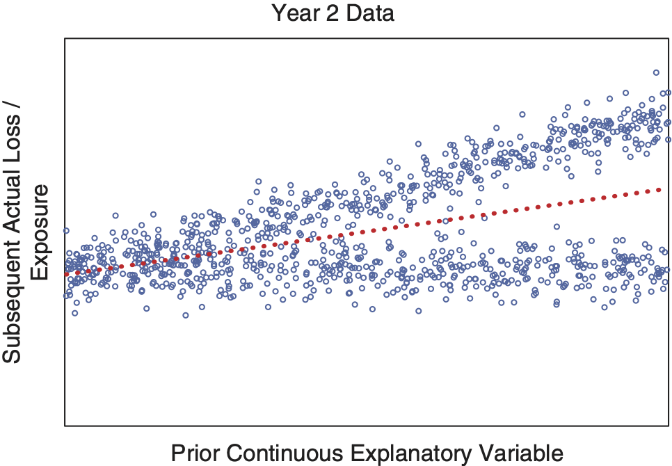
Figure 2.2 displays a data cloud in which the vertical axis is the actual loss per exposure subsequent to information available about an explanatory variable shown by the horizontal axis, along with a dotted regression line. Figures 2.3 and 2.4 show the corresponding data clouds for Year 1 and Year 2, respectively. It is clear that the same forked pattern appears in each year, as well as when the years are combined. However, this pattern clearly seriously violates many of the previously mentioned standard assumptions for linear regression:

• ξ is clearly not normal.

• σ² is not constant.

• ξ is dependent on X.

Figure 2.5 shows a bootstrap quintile test using the regression line from Year 1 to predict Year 2. Despite violating the assumptions, predictive performance for the expected loss rate in Year 2 based on the explanatory variable is excellent, and the model would be very useful in practice.

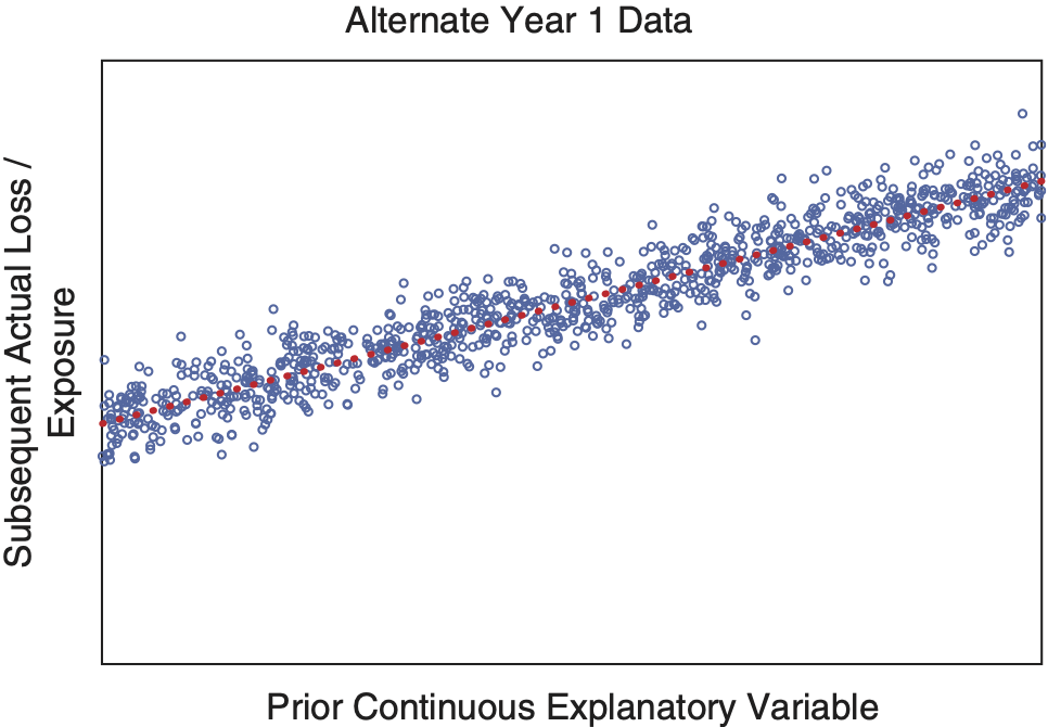
Figures 2.6 and 2.7 show an alternative composition by Year 1 and Year 2 of the same combined data shown in Figure 2.2. In this alternative situation, both Year 1 and Year 2 demonstrate patterns that are clearly consistent with the assumptions of linear regression, but the slope has changed significantly from Alternative Year 1 to Alternative Year 2. Figure 2.8 shows a bootstrap quintile test using the regression line from Alternative Year 1 to predict Alternative Year 2. Despite obeying the linear regression assumptions in each year, the model’s predictive performance is terrible. In fact, it is so bad that it would be much better to simply predict a 0 slope for Alternative Year 2.

Note that in a real-world application of a predictive framework, the performance of the regression line from the first year to predict the second year would be tested. If it performed well, then the regression line for the second year would be used to forecast a third year. So predictive performance testing would result in utilizing the regression line in the first case but discarding it in the alternative case. The real-world loss process would most likely lead to the third year resembling the second year in the first situation, but having a different slope from that of the second year in the alternative situation. Consequently, predictive performance testing would work well by obtaining predictive value when it is available but avoiding the pitfall of a poor prediction.

In contrast, in a more traditional statistical framework, typically the combined first- and second-year data would be tested for the assumptions of linear regression. The assumption testing would obviously fail, and the regression would be discarded. This would avoid the poor predictive performance in the alternative case but also miss the high predictive value for the first case. However, if it so happened that the assumption testing were performed only on the second-year data in the alternative situation, in which the assumptions would be valid for that year, the regression would be used, resulting in poor predictive performance for the third year.

3. Multiplicative minimum bias iteration

Suppose the basic data available consist of aggregated actual losses $L_{i_{1},\ldots,i_n}$ ≥ 0 and exposures $P_{i_{1},\ldots,i_n}$ ≥ 0, ($P_{i_{1},\ldots,i_n}$ = 0 ⇒ $L_{i_{1},\ldots,i_n}$ = 0), where i_j = 1, . . . , n_j indexes the individual classes within the classification dimension j, and i₁,..,i_n denotes the cell corresponding to the intersection of a single class selected in each classification dimension. Also, the total exposure in any class is positive, $\sum_{i_{j}=k}P_{i_{1},\ldots,i_n}$ > 0; otherwise it would make sense to exclude the class entirely from estimating rating parameters. A multiplicative minimum bias model assumes that $L_{i_{1},\ldots,i_n}$ = $B_{i_{1},\ldots,i_n}$ + $P_{i_{1},\ldots,i_n} \prod_{j=1, \ldots, n_{j}} X_{j, i, j}$. The parameters $X_{j,i_j}$ are fitted with the goal of minimizing some bias function, or functions, of the residual errors $B_{i_{1},\ldots,i_n}$.

The minimum bias goal is that the sum of the residual errors for each class $\sum_{i_{j}=k} B_{i_{1},\ldots,i_n}$ should be 0. A corresponding iterative sequence of parameter estimates can be formed whose convergence corresponds to convergence toward that goal:

$$\begin{aligned} X_{j, k, 1} & =1 \\ X_{j, k, t+1} & =\frac{\sum_{i_{j}=k} L_{i_{1}, \ldots, i_{n}}}{\sum_{i_{j}=k} P_{i_{1}, \ldots, i_{n}} \prod_{l \neq j} X_{l, i_{l}, t}} . \end{aligned}$$

The effective sample is now $\sum_{j=1, \ldots, n} n_{j}$ data points with values $\sum_{i_{j}=k} L_{i_{1},\ldots,i_n}$, which reduces to $\sum_{j=1, \ldots, n} n_{j}$ − (n − 1) linearly independent numbers. There is a corresponding (n − 1) dimensional degeneracy in the parameters. If the parameters $X_{k,i_k}$ are multiplied by a constant c > 0 and the parameters $X_{l,i_l}$ are divided by c, where 0 ≤ k < l ≤ n, then will be unchanged.

The central limit theorem implies that the distribution of $\sum_{i_{j}=k} L_{i_{1},\ldots,i_n}$ can be expected to more closely resemble a normal distribution, with a generally lower coefficient of variation than the individual cell values $L_{i_{1},\ldots,i_n}$. However, whereas the cellular values $L_{i_{1},\ldots,i_n}$ can reasonably be assumed to be statistically independent of each other, the further aggregated values $\sum_{i_{j}=k} L_{i_{1},\ldots,i_n}$ include many statistical dependencies, since there is an overlap of cells between classes in different dimensions. So a trade-off is made for a minimum bias iteration model. Statistical independence of sample data points, a desirable property, is partially sacrificed in exchange for the benefit of a more normal distribution, generally having a lower coefficient of variation than the distributions underlying each sample data point. This taming of the distribution of data points means that it becomes less necessary to specify the distribution of the individual cellular loss values or, as may be the case, the distributions of individual loss observations within the cells, as would be necessary for a GLM.

Example 2

Suppose there are three classification dimensions, each with 10 classes, resulting in 1,000 individual cells. We can expect about 100 times as much data volume underlying each class as for each cell, and correspondingly an average coefficient of variation by class that is only about 10% as much as by cell. Two classes in different dimensions overlap in 10 cells, and thus actual losses between them will have a correlation coefficient of about 10%.

Multiplicative minimum bias effectively aims toward the same parameter estimates as a GLM with a logarithmic link function and Poisson likelihood function. The logarithmic link converts the sum of linear explanatory factors into a multiplicative product of their exponentials. The Poisson likelihood leads to equations for MLE that correspond to a fixed limit point of the minimum bias iteration, as pointed out by Brown (1988).

However, the Poisson distributional assumption is usually unrealistic and not a part of the minimum bias model. Data are generally not restricted to integer values. The Poisson coefficient of variation is not scale independent (e.g., it is 10 times greater when applied to dollar amounts than when applied to the same amounts measured as pennies) and implodes for large nominal means (e.g., a mean of 1 million implies a coefficient of variation of 0.1%). So the Poisson assumption is important only in the optimization equations it implies for MLE.

4. Incorporating credibility

Credibility adjustments, 0 ≤ $Z{j,i_j}$ ≤ 1, can be easily and directly incorporated into the iteration equations:

$$\begin{aligned} X_{j, k, 1}= & 1 \\ X_{j, k, t+1}= & Z_{j, k} \frac{\sum_{i_{j}=k} L_{i_{1}, \ldots, i_{n}}}{\sum_{i_{j}=k} P_{i_{1}, \ldots, i_{n}} \prod_{l \neq j} X_{l, i, t}} \\ & +\left(1-Z_{j, k}\right) \frac{\sum L_{i_{1}, \ldots, i_{n}}}{\sum P_{i_{1}, \ldots, i_{n}} \prod_{l \neq j} X_{l, i, t}} . \end{aligned}$$

Note that, other than the constraint of the interval [0, 1], nothing has been specified about the determination of Z_j,i. There are many possibilities for $Z_{j,i_j}$, including functions of the sum of exposure, P_j,k = $\sum_{i_{j}=k} P_{i_{1},\ldots,i_n}$. The ultimate test will be the predictive performance of the final model regardless of whether Z_j,i itself satisfies any traditional goals of credibility theory, such as limiting fluctuation or having the greatest accuracy.

For GLM, the basic and common protection against fitting parameters to data that are not credible is to throw away explanatory variables whose parameters are not statistically distinct from 0, those variables with high p-values.

To add true credibility, or “shrinkage,” adjustment is complicated. The two main approaches are these:

1. General linear mixed models. At least some rating factors are assumed to be random rather than fixed effects, but an MLE-like fitting method is still used. Numerical solution is rather difficult and, in practice, functions in R or procedures in SAS are used, effectively as black boxes. See Frees, Derrig, and Meyers (2014); Klinker (2001); and Nelder and Verrall (1997) for background.

2. Bayesian networks and Gibbs sampling. Rating factors in each class dimension follow a prior distribution. The parameters of the prior distributions follow distributions that are very diffuse. Numerical solution is performed using a Gibbs sampling program, such as JAGS or WinBUGS. The model itself is elaborately specified and lucid to an audience sophisticated enough read the specification. See Frees, Derrig, and Meyers (2014) and Scollnik (1996) for background.

In Section 7, we will demonstrate an example of the second approach.

5. Anchoring and iteration blending for practical iterative convergence

In practice, the convergence of the iterative algorithms can be a problem even after the application of credibility. For one thing, there is still the problem of (n − 1) dimensional degeneracy previously mentioned. Also, highly correlated dimensions can contribute to nonconvergence or slow convergence in practice. Other than the automatic degeneracy, we will not attempt to deal in a precise mathematical way with the more general convergence issue, which appears to be an open problem for multiplicative minimum bias. From a practical point of view, anchoring and iteration blending can effectively provide timely convergence.

Anchoring directly eliminates the degeneracy. One approach is to fix one of the class parameters in each of (n − 1) classification dimensions to the value of 1.0, or to fix such a parameter in each of n dimensions and add a single overall base rate parameter. Another approach is to use a single overall base rate and rescale the parameters in each dimension to a weighted average of 1.0 at the end of each iteration.

Example 3

If P = $\left(\begin{array}{ll} 1 & 1 \\ 1 & 1 \end{array}\right)$ and L = $\left(\begin{array}{ll} 1 & 2 \\ 3 & 4 \end{array}\right)$, then parameter iterations will oscillate back and forth between the values X = $\left(\begin{array}{ll} 1.5 & 3.5 \\ 2.0 & 3.0 \end{array}\right)$ and X = $\left(\begin{array}{ll} 0.6 & 1.4 \\ 0.8 & 1.2 \end{array}\right)$. However, if we anchor one parameter at 1.0, the iterations will converge to X = $\left(\begin{array}{ll} 1.000 & 2.333 \\ 1.200 & 1.800 \end{array}\right)$.

Iteration blending can be implemented to accelerate convergence by modifying the iterative equations to be

$$\begin{aligned} X_{j, k, t+1}= & \alpha\left[\begin{array}{c} \sum_{j, k} \frac{L_{i_{j}=k} L_{i, \ldots, i_{n}}}{\sum_{i_{j}=k} P_{i_{1, \ldots}, \ldots, i_{n}} \prod_{l \neq j} X_{l, i, t}} \\ +\left(1-Z_{j, k}\right) \frac{\sum L_{i_{i, \ldots, i_{n}}}}{\sum P_{i_{1, \ldots, \ldots, i_{n}} \prod_{l \neq j} X_{l, i, t}}} \end{array}\right] \\ & +(1-\alpha) X_{j, k, t-1}, \end{aligned}$$

where 0 < α < 1 is a selected constant blending parameter.

As an extreme illustration of correlation, let one classification dimension be replicated or made once redundant. Setting α = 0.5 will allow the model to converge. Each one of the replicated dimensions will end up sharing equally in the observed predictive relationship, combining together to provide the appropriate prediction. In the case of full credibility, they will exactly reproduce the result obtained from not replicating the dimension. With less than full credibility, the result will not be exactly the same as that obtained from not replicating the dimension, but it will be similar.

6. Testing of individual explanatory variables

Sometimes predictive modeling techniques are used specifically to determine whether or not individual explanatory variables, or equivalent classification dimensions, are statistically significant. As mentioned earlier, when using GLM techniques, it is common to consider the p-values of the estimated parameters. These p-values are calculated under the distributional and other assumptions, such as independence of the GLM model being used.

Whether distributional assumptions are made (as with GLM) or not (as with minimum bias), tests of predictive performance can be performed and compared, with and without a given classification dimension. In cases where the improvement is insignificant, the dimension should be removed for the sake of parsimony.

7. Empirical case study

The empirical data used in this case study consist of 371,123 records of medical malpractice payments obtained from the National Practitioner Data Bank. Three explanatory variables will be used for modeling payment amounts: Origination Year, Allegation Group, and License Field. The records will be randomly split into two sets, for model fitting and validation, respectively. Further details are included in Appendix A.

7.1. GLM model specifications

For our GLM model, we will consider the following:

1. The logarithmic link function, which causes the fit factors to act multiplicatively.

2. Several likelihood functions: Gaussian, Poisson, gamma, and inverse Gaussian. These correspond to assumptions that variance σ² is related to mean μ as σ² = constant, σ² ∝ μ, σ² ∝ μ², and σ² ∝ μ³, respectively.

3. Initially we will ignore credibility considerations, aside from reviewing p-values, and later we will use Gibbs sampling to incorporate credibility.

4. The GLM will be fitted, as is customary, to the individual data records without aggregation into cells based on intersections of the explanatory variables, as happens for the minimum bias model.

7.2. Comparison of GLM and minimum bias model results

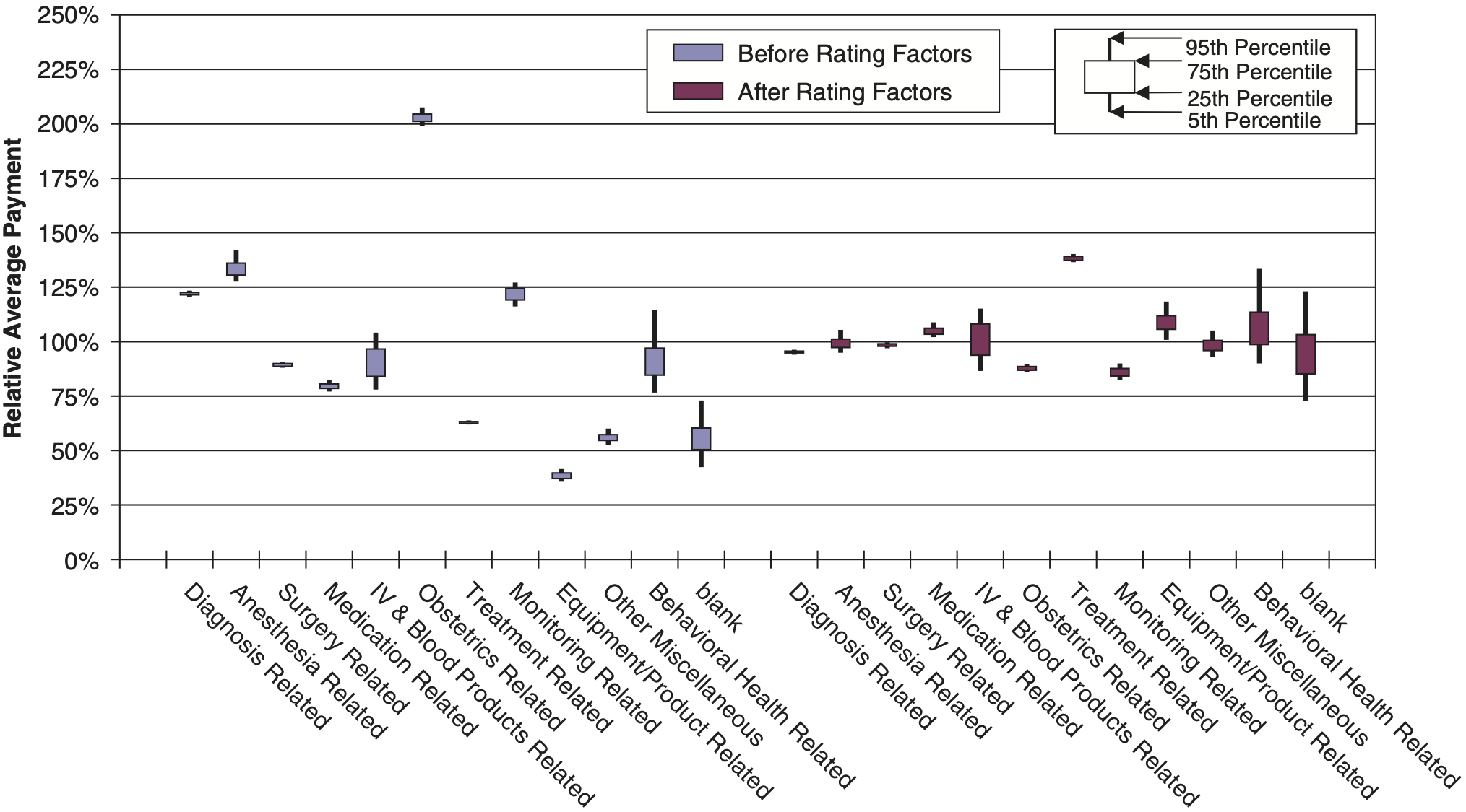
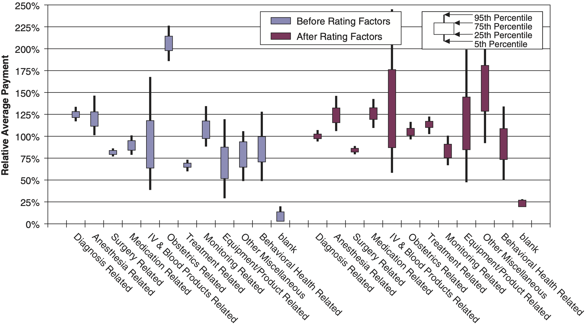
Figures 7.1 and 7.2, and Table 7.1, show the bootstrap quantile testing results of the fitting and the performance testing models. Optimal noise-to-signal estimates along the lines described in Evans and Dean (2014) suggested using 20 quantiles. Also, see Evans and Dean (2014) for details on the definitions of the test statistics. The “old statistic” test measure is the ratio of the variance of the relative average payments after rating factors are applied, to the same variance before rating factors are applied, lower being better. For example, an “old statistic” value of 0.200 can be intuitively interpreted as indicating that the rating factor has eliminated or “flattened out” 80% of the difference in relative losses that it detected. The “new statistic” test measure is essentially the square root of the difference between these two variances, higher being better. For example, a “new statistic” value of 0.300 can be intuitively interpreted as indicating that the rating factor has typically reduced the relative differences between quantiles (or, if applicable, categories) by 30% (e.g., two categories with relative loss ratios of 80% and 130% might have something closer to 90% and 110%, respectively, for relative loss ratios after the rating factor is applied).

Although Figures 7.1 and 7.2 correspond only to the minimum bias fits, Table 7.1 demonstrates that the log-Poisson GLM was identical to the minimum bias approach, and the best-fitting model. In fact, we checked the individual predicted values and verified that they were numerically identical. Log-Gaussian and log-gamma were almost as good. The MLE for our run of log–inverse Gaussian failed to converge, almost certainly driven by its unrealistic variance assumption.

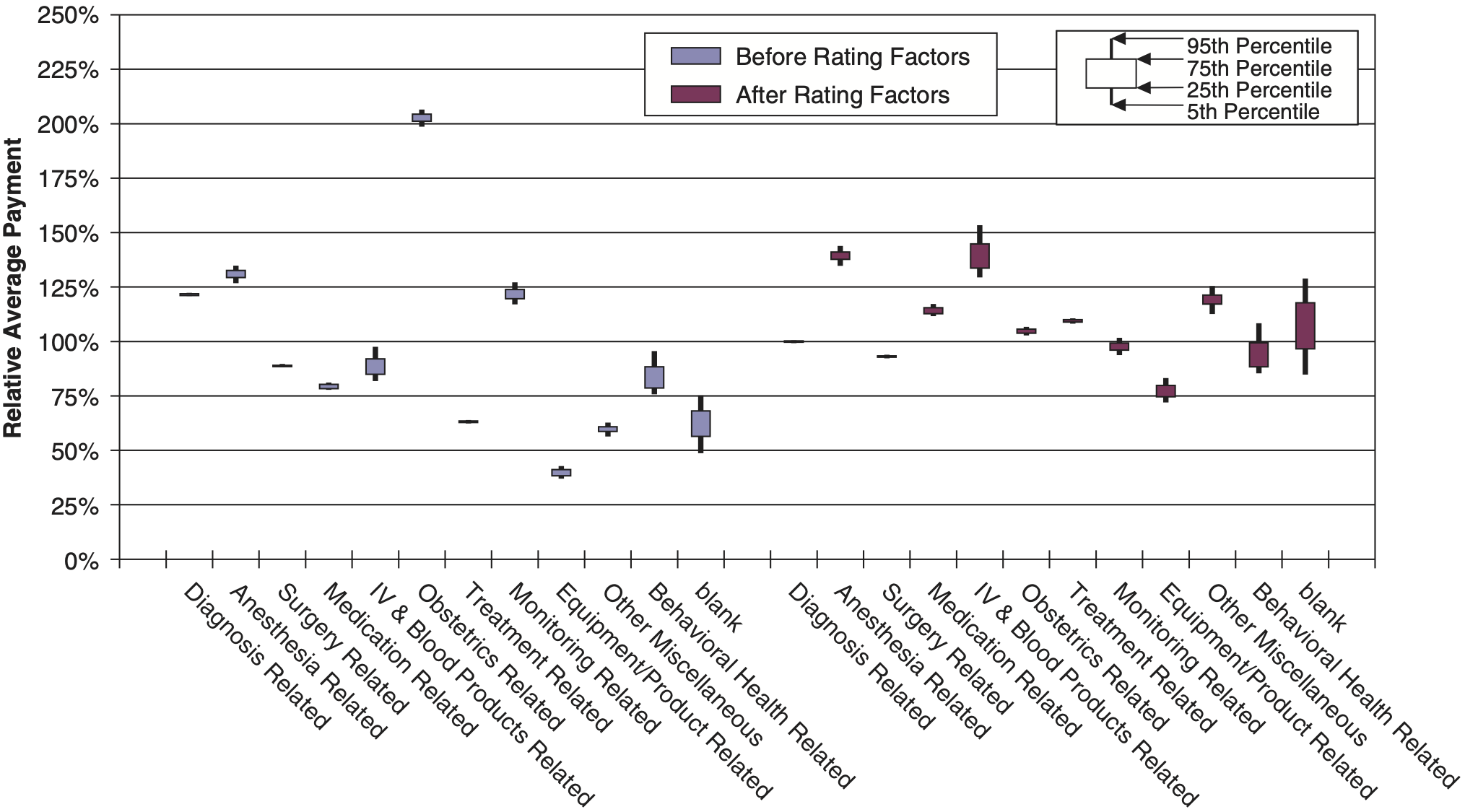
Figures 7.3 and 7.4 correspond to “traditional” univariate rate relativities for the three explanatory variables. Rating factors are calculated separately and independently in each classification dimension. The traditional method clearly performs much worse than minimum bias and the convergent GLMs, but it is still a great improvement over no adjustment.

At this point we have a clear picture of the relative predictive performance of the different models. However, we have not specifically tested the validity of any of the model assumptions, such as likelihoods, independence assumptions, etc. The optimal performance of minimum bias / log-Poisson is likely due to the general validity of its implicit connection to the central limit theorem, as discussed earlier.

The GLM assumption that all risks are identically distributed is potentially problematic when taken together with the log-link function.

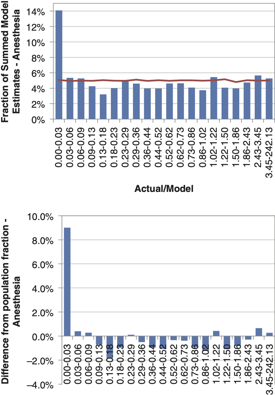
Figures 7.5 through 7.7 illustrate the lack of distributional consistency for this dataset. We have broken the observations in the training data into 20 quantiles weighted by modeled values, sorted by actual versus modeled result. Using the same breakpoints, determined from the entire training dataset, we then calculated the summed modeled values for each allegation group. If the errors were identically distributed for each allegation group, there should be only a random fluctuation, around the 5% of total expected for each bin.

Figure 7.5 shows all allegation groups and, naturally, each bin demonstrates no differences in the weighted proportion. Figure 7.6 shows that the anesthesia-related allegation group has a much higher percentage of the error distribution in the lowest bin than what would be expected from the overall population. Figure 7.7 shows that, while not as dramatic, the treatment-related allegation group shows greater variation than the overall error distribution, with more of the highest and lowest values.

This is far from uncommon with highly skewed insurance data. The problem is compounded by the multiple dimensions of data. Error distributions could be, and likely are, differently distributed across many of the dimensions, if not every dimension being analyzed. Without adjustment, the basic assumption in a GLM is that the errors are identically distributed. The use of the log-link function, in conjunction with maximum likelihood estimation, puts a great deal of faith in the distributional assumption, inferring conclusions about results in the tail, based on the more voluminous observations at the lower parts of the distribution. But it is the tail itself that is of primary interest in most insurance questions, with the majority of the aggregate losses being caused by the minority of claims. Despite the unreasonable implied assumption of a log-Poisson GLM, because it happens to have effectively the same parameter estimation formulas as the multiplicative minimum bias approach, which has the advantages of the associated central limit theorem (as previously described), it is less vulnerable to these distributional differences.

Table 7.2 shows a comparison of the model biases by allegation group on the validation data using multiplicative minimum bias with full credibility versus GLM with a log-Gaussian assumption. To do so, it compares actual aggregated results by allegation group with aggregated modeled results over a number of bootstrapped test sets. Despite the log-Gaussian assumption’s better characterizing the distribution of the data than does the log-Poisson assumption, it ultimately produces estimates that are more vulnerable to distributional differences. The only allegation group with a worse log-Gaussian mean bias is that of equipment/product-related payments, and in that group, both sets of bootstrapped ranges contain 0, suggesting that the bias measure is inconclusive.

7.3. Incorporating credibility into minimum bias

Although the overall predictive performance without any credibility adjustments was very good, there are reasons to explore credibility. In some sparsely populated classes for License Field, rating variables might be so unreliable as to lead to adverse selection problems in real-world applications.

In the previous example, the p-values for the rating factors in the log-Poisson were all infinitesimally low (the largest p-value ∼ 10⁻²⁰⁴). This is likely due to the problematic general phenomenon that p-values always tend to implode with very large volumes of data, such as the volume in the example. In stark contrast, most of the p-values for the log-Gaussian and log-gamma models were high, from 1% to approaching 100%. Whether these p-value results indicate that any of the likelihood selections are valid, or whether they do not, they demonstrate the generally awkward nature of trying to use p-values and class consolidation to handle the lack of credibility in sparsely populated classes.

Rather than attempt a p-value-based class consolidation, we will explore the impact of a very simple credibility adjustment for minimum bias. We select the very simple form $Z_{j, i_{j}}=\frac{P_{j, i_{j}}}{P_{j, i_{j}}+K}$, where $P{j,i_j}$ is the number of records in which the i_j class for classification dimension j and K ≥ 0 is a judgmental selection. Table 7.3 shows that this simple credibility adjustment tends only to erode overall predictive value for this large dataset, with only truly predictive variables included.

To construct a smaller example in which credibility is more relevant, we will use a random set of only 5,000 records for fitting and another random set of 5,000 records for testing, shown in Tables 7.4 and 7.5 and Figures 7.8 through 7.11. We will also do a full test using all the remaining 366,123 records not used for fitting, shown in Tables 7.6 and 7.7 and Figures 7.12 and 7.13.

As Tables 7.4 through 7.7 and Figures 7.8 through 7.12 show, the incorporation of credibility was particularly important when distinguishing differences between the allegation groups. Actuaries are regularly asked to provide estimates of the impact of rating variables despite having less than fully credible data. While the overall result may appear to be relatively unaffected by increasing the credibility standard, the ability to differentiate between them more robustly is illustrated.

7.4. Incorporating credibility into GLM

We can incorporate credibility, or “shrinkage” of parameter estimates, into a GLM model by defining a hierarchical Bayesian network of random variables:

1. U_1,j = 0 j = 1, 2, 3

2. U_1,4 = Uniform(0, 20)

3. U_i,1 ∼ Normal(−σ₁²/2, σ₁²) i = 2, . . . , 83

4. U_i,2 ∼ Normal(−σ₁²/2, σ₁²) i = 2, . . . , 12

5. U_i,3 ∼ Normal(−σ₁²/2, σ₁²) i = 2, . . . , 9

6. σ₁² ∼ Lognormal(0, 10)

7. σ₂² ∼ Lognormal(0, 10)

8. δ_k ∼ Normal(−σ₂²/2, σ₂²) k = 1, . . . , n

9. Y_k ∼ Poison(Exp(δ_k + U_1,4 + $U_{i_{1,k},1}$ + $U_{i_{2,k},2}$ + $U_{i_{3,k},1}$))
   k = 1, . . . , n

Y_k are the individual actual claim amounts to be fitted. U_i,j are parameters in log space, with U_1,4 being a constant and the other j = 1, 2, or 3, corresponding to License Field, Allegation Group, and Origination Year, respectively. i_j,k is an index of which class the Y_k observation falls into in each classification dimension. δ_k is a random overdispersion for each observation, which itself has variance σ₂². σ₁² is the parameter variance for each class parameter. Since U_1,4, σ₁², and σ₂² follow highly diffuse distributions, they will effectively be “fitted” parameters when Gibbs sampling is performed. σ₁² and σ₂² conceptually correspond to parameter and process variances in credibility, respectively.

We also defined a simpler form of this model, eliminating the overdispersion arising from σ₁² and σ₂². Running this simpler model numerically produced the same parameters as the MLE log-Poisson/minimum bias with no credibility adjustment, confirming that our Gibbs sampling model is constructed and coded on the right track up to the point of adding credibility adjustments.

When the model including the δ_k and σ₂² was run numerically, we observed a shrinkage effect in the set of parameters. Table 7.8 shows that the range of the U_i,1 contracted significantly with overdispersion. There was a slight broadening of the ranges for U_i,2 and U_i,3, which is not unreasonable, as none of the corresponding classes in these dimensions are sparsely populated.

Unfortunately, although there was a credibility-like shrinkage effect, the predictive performance actually deteriorated. Figures 7.14 and 7.15 show the deteriorating situation when the Gibbs sampling with overdispersion is included in the large split of the data. Table 7.9 shows the deterioration in test statistics for both the large split and the smaller sample.

There are potential criticisms of the Bayesian network model as we have defined it—for example, anchoring the parameters for the first classes U_{1, j} = 0 j = 1, 2, 3; offsetting the prior distributions on parameters so as to have mean 1 after exponentiation U_i,1 ∼ Normal(−σ₁²/2, σ₁²) i = 2, . . . , 83; using the same parameter variance, σ₁², for all three classification dimensions; etc. However, the authors experimented with a myriad of alterations to the model definition, even going so far as to convert the likelihood function into a negative binomial distribution to capture the impact of overdispersion of the Poisson more directly. In all cases, predictive performance deteriorated further or did not improve. The previously presented multiplicative minimum bias model with incorporated credibility would be vulnerable to similar or more extensive potential criticisms. Yet implementing it went quickly, and it easily produced desirable results.

This failed modeling experience in no way proves that a well-performing Gibbs-sampled Bayesian model cannot be defined in this context. Obviously, well-performing examples for much simpler situations, such as one classification dimension and an identity link function, are well known and easy to construct. Nor is the point that the theory behind these models does not provide deep insights into understanding modeling and statistical estimation. However, in this case, orders of magnitude more input of resources, both in time and sophistication of effort, than was used for minimum bias produced inferior predictive performance. Though neither author of this paper is a specialist in Gibbs sampling methods, one author (Evans) has used them occasionally for over 10 years and informally consulted several specialists with more experience (in Acknowledgments). As of this writing, we have not been able to diagnose why the model as defined performs so much more poorly than a regular MLE GLM with no shrinkage effect. Whether the model is in some way poorly designed or, much less likely, one of the many technical choices made in running the Gibbs sampling software should be tuned differently does not alter the key conclusion, namely, that the tremendous additional resource and intellectual burdens of such detailed and sophisticated models may offer no advantage, or may even be disadvantageous, in many practical situations of predictive modeling.

8. Summary discussion

The predictive modeling framework greatly reduces the burdens of model specification, because models are validated based on their predictive performance rather than hypothesis testing of model assumptions. Minimum bias models transform basic data in such a way as to partially sacrifice sample independence in exchange for much tamer distributions of aggregated individual data points that are much less needy of detailed distributional specification. The combination of multiplicative minimum bias iteration with a generic incorporation of credibility, as presented in this paper, demonstrates that a very simple model, without complete distributional specification, in practice may provide predictive value comparable to or better than that of a far more complex model, such as a typical GLM or, particularly, a GLM adjusted to incorporate credibility.

GLM models are fitted to individual data points and require specification of the distributions underlying each data point. Consequently, GLM models can be significantly vulnerable to inaccurate specifications, and their fundamental complexity makes the practical incorporation of credibility adjustments, such as including random effects or fitting parameters through Gibbs sampling, very complex.

Philosophically, simpler modeling is desirable. In practice, simpler models are beneficial in many ways, such as lower skill requirements for operational personnel and greater lucidity to a much wider audience. Some previous papers, such as those by Brown (1988) and Mildenhall (1999), have highlighted the sense in which minimum bias iteration is a special case of GLM and encouraged—at least implicitly—minimum bias practitioners to switch to GLM as a richer framework. There is some irony that with the advent of the predictive framework, minimum bias may often be somewhat more advantageous, in principle and practice. However, it should be emphasized that this does not mean that the detailed specifications of a particular GLM might not produce superior predictive performance in a situation where the process underlying the data closely matches the particular assumptions of that GLM.

While GLM models are powerful and belong in the set of tools applied by actuaries, consideration should also be given to multiplicative minimum bias models and the traditional actuarial concept of partial credibility. Ultimately the test of any predictive model should be how it performs on out-of-sample data.

---

Acknowledgments

The authors are thankful to Jose Couret, Louise Francis, Chris Laws, and Frank Schmid for answering some questions that arose in the course of writing this paper.

model
{
 U[1,4]∼dunif(0,20)
 U[1,1]<-0
 U[1,2]<-0
 U[1,3]<-0
 Tau[1] ∼ dlnorm(0,0.1)
 Mu<- -pow(Tau[1],-1)/2
 Tau[2] ∼ dlnorm(0,0.1)
 Mu2<- -pow(Tau[2],-1)/2
 Tau[3]<-Tau[1]/Tau[2]
 for(i in 2:N1) { U[i,1]∼dnorm(Mu,Tau[1]) }
 for(i in 2:N2) { U[i,2]∼dnorm(Mu,Tau[1]) }
 for(i in 2:N3) { U[i,3]∼dnorm(Mu,Tau[1]) }
 for(i in 1:N) {
  ProcError[i]∼dnorm(Mu2,Tau[2])
  lambda1[i]<-exp(min(20,ProcError[i]+U[1,4]
    +U[X[i,1],1]+U[X[i,2],2]+U[X[i,3],3]))
  Y[i]∼dpois(lambda1[i])
  }
}

model
{
 U[1,4]∼dunif(0,20)
 U[1,1]<-0
 U[1,2]<-0
 U[1,3]<-0
 Tau[1] ∼ dlnorm(0,0.1)
 Mu<- -pow(Tau[1],-1)/2
 for(i in 2:N1) { U[i,1]∼dnorm(Mu,Tau[1]) }
 for(i in 2:N2) { U[i,2]∼dnorm(Mu,Tau[1]) }
 for(i in 2:N3) { U[i,3]∼dnorm(Mu,Tau[1]) }
 for(i in 1:N) {
  lambda1[i]<-exp(min(20,U[1,4]+U[X[i,1],1]+
      U[X[i,2],2]+U[X[i,3],3]))
  Y[i]∼dpois(lambda1[i])
  }
}