An Empirical Investigation of the Value of Claim Closure Count Information to Loss Reserving

undefined

1. Introduction

1.1. Background and purpose

The data set provided by Meyers and Shi (2011) makes available a large number of US claim triangles for experimentation in loss reserving. The triangles are of two types, namely:

• Paid claims; and

• Incurred claims.

Triangles of these types are suitable for analysis by the chain ladder model, and indeed this is very common in practice. Some jurisdictions across the globe are accustomed to the use of alternative loss reserving models (see, e.g., Taylor (2000)). Commonly, these alternatives rely on additional data, particularly triangles of counts of reported claims and finalized claims, respectively.

This raises the question as to reasons Meyers and Shi did not collate count data. In private correspondence the authors advised that they had sought the views of other US actuaries on this very matter and had been counseled not to do so.

Count data, particularly claim closure counts, were said to be unreliable. There was more than one reason for this. First, some portfolios included material amounts of reinsurance, and the meaning of claim closure was not clear in all of these cases. But more than this, it appears that such counts are not always returned by insurers with all diligence and are unreliable on that account.

Moreover, the models that rely on count data have not received universal acclaim. Some statisticians have commented adversely, noting that these models, requiring more extensive data, also require more modeling, more parameterization, leading to more uncertainty in forecasts.

This argument cannot be correct as a matter of logic. If claim closure counts followed a deterministic process, they would add no uncertainty, and the argument would fail. If they follow a process with a very small degree of stochasticity, then they would add little uncertainty, and again the argument would fail.

The evident question of relevance is whether any reduction in uncertainty in the claim payment model by conditioning on the count data is more than, or less than, offset by the additional uncertainty induced by the modeling and forecasting of the counts themselves.

The forecasts of some claim payment models that rely on claim closure count data are relatively insensitive to the distribution of claim closures over time. So any uncertainty in the forecast of this distribution will have little effect on the forecast of loss reserve in this case. These models are the operational time models, as discussed in Section 4.3.

The debate on the merits of these models relative to the chain ladder appears fruitless. It might be preferable to allow the data to speak for themselves. That is, forecast according to both models, estimate prediction error of each, and select the model with the lesser prediction error.

Much the same argument can be applied to the issue of reliability of count data. The data may be allowed to speak for themselves by the use of prediction error as the criterion for model selection. Data unreliability should be found out through an enlarged prediction error.

The purpose of the present paper is to compare loss reserving models that rely on claim count data with the chain ladder model, which does not rely on counts. It is equally important to state what the purpose of the paper is not. The objective is not to criticize the chain ladder, which bears a long pedigree, and is seen to function perfectly well in many circumstances.

The objective is rather to focus on specific circumstances in which a priori reasoning would suggest that the chain ladder’s prediction performance might be suspect, and to examine the comparative performance of alternative models that rely on claim counts.

Chain ladder failures have been observed in the literature. For example, Taylor (2000) discusses an example in which the chain ladder estimates a loss reserve that is barely half that suggested by more comprehensive analysis. As another example, Taylor and McGuire (2004) discuss a data set for which modification of the chain ladder to accommodate it appears extraordinarily difficult. In both examples, the chain ladder failure was seen to relate to changing rates of claim closure.

The chain ladder model, as discussed in this paper, is of a fixed and inflexible form that leads to the mechanical calibration algorithm set out in Section 4.1.2. This model is based on specific assumptions that are discussed in Section 4.1.3, and these assumptions may or may not be sustainable in specific practical cases.

In practice, actuaries are generally aware of such shortcomings of the model and take steps to correct for them. The sorts of adjustments often implemented on this account are discussed briefly in Section 4.1.4, where it is noted that they often rely heavily on subjectivity.

It is desirable that any comparison of the chain ladder with contending alternatives should, for the sake of fairness, take account of those adjustments. In other words, comparison should be made with the chain ladder, as it is actually used in practice, rather than with the textbook form referred to above.

Unfortunately, such comparisons do not fit well within the context of controlled experiments. Any attempt to implement subjective forms of the chain ladder would almost certainly shift discussion of the results into controversy over the subjective adjustments made.

In any event, the mode of comparison of a subjective model with other formal models is unclear. Model comparison is made in the present paper by means of estimates of prediction error. These can be computed only on the basis of a formal model. Further comment is made on this point in Section 7.

In light of clear alternatives, comparison is made here between the “basic,” or “classical,” form of the chain ladder and various contending models. This might be seen as subjecting the chain ladder to an unjustified disadvantage in the comparisons. Some countervailing considerations are put in Section 7, but in the final analysis it must be admitted that the results of the model comparisons herein are not entirely definitive. This strand of discussion is also continued in Section 7.

1.2. The use of claim counts in loss reserving

The motivation for the use of claim counts in loss reserving commences with some simple propositions:

• that if, for example, one accident year generates a claim count equal to double that of another year, then the first accident year might be expected to generate an ultimate claim cost roughly double that of the second year;

• that if, for example, the count of open claims from one accident year at the valuation date is equal to double that of a second accident year at the same date, then the amount of outstanding losses in respect of the first year might be expected to equal roughly double the amount in respect of the second year.

If loss reserving on the basis of a model that does not take account of claim counts is observed to produce conclusions at variance with these simple propositions, then questions arise as to the appropriateness of that model. The model may remain appropriate in the presence of this conflict, but the reasons for this should be understood.

One possibility is that the model is in fact inappropriate to the specific data set under consideration. In this case, formulation of an alternative model will be required, and it is possible that the alternative will need to include terms that depend explicitly on the claim counts.

For example, a model based on the second of the propositions cited above may estimate the outstanding losses of an accident year as the product of:

• the estimated number of those outstanding losses (including IBNR); and

• their estimated average severity (i.e., average amount of unpaid liability per claim).

This approach was introduced by Fisher and Lange (1973) and rediscovered by Sawkins (1979). One approach to it, the so-called Payments Per Claim Finalized model (PPCF), is described by Taylor (2000, Section 4.3). The premise of this model is that, in any cell of the claims triangle, the expectation of paid losses will be proportional to the number of closures.

This renders the model suitable for lines of business in which loss payments are heavily concentrated in the period shortly before claim closure. Auto Liability and Public Liability would usually fit this description. Workers Compensation would also, in jurisdictions that provide for a high proportion of settlements by common law, but less so with an increasing proportion of payments as income replacement installments.

2. Framework and notation

2.1. Claims data

Consider a J × J square of claims observations Y_kj with:

• accident periods represented by rows and labeled k = 1, 2, . . . , J;

• development periods represented by columns and labeled by j = 1, 2, . . . , J.

For the present the nature of these observations will be unspecified. In later sections they will be specialized to paid losses, reported claim counts, unclosed claim counts or claim closure counts, or even quantities derived from these.

Within the square identify a development triangle of past observations,

$$\mathfrak{D}_{J}=\left\{Y_{k j}: 1 \leq k \leq J \text { and } 1 \leq j \leq J-k+1\right\} .$$

Let ℑ_J denote the set of subscripts associated with this triangle, i.e.,

$$\Im_{J}=\{(k, j): 1 \leq k \leq J \text { and } 1 \leq j \leq J-k+1\}$$

The complement of this subset, representing future observations is

$$\mathfrak{D}_{J}^{c}=\left\{Y_{k j}: 1 \leq k \leq J \text { and } J-k+1<j \leq J\right\} .$$

Also let

$$\mathfrak{D}_{J}^{+}=\mathfrak{D}_{J} \cup \mathfrak{D}_{J}^{c}$$

In general, the problem is to predict 𝔇^c_J on the basis of observed 𝔇_J.

Define the cumulative row sums

$$Y_{k j}^{*}=\sum_{i=1}^{j} Y_{k i} \tag{2.1}$$

and the full row and column sums (or horizontal and vertical sums) and rectangle sums

$$\begin{array}{l} H_{k}=\sum_{j=1}^{J-k+1} Y_{k j} \\ V_{j}=\sum_{k=1}^{J-j+1} Y_{k j} \\ T_{r c}=\sum_{k=1}^{r} \sum_{j=1}^{c} Y_{k j}=\sum_{k=1}^{r} Y_{k c}^{*} . \end{array} \tag{2.2}$$

Also define, for k = 2, . . . , J,

$$R_{k}=\sum_{j=J-k+2}^{J} Y_{k j}=Y_{k J}^{*}-Y_{k, J-k+1}^{*} \tag{2.3}$$

$$R=\sum_{k=2}^{J} R_{k} . \tag{2.4}$$

Note that R is the sum of the (future) observations in 𝔇^c_J. It will be referred to as the total amount of outstanding losses. Likewise, R_k denotes the amount of outstanding losses in respect of accident period k. The objective stated earlier is to forecast the R_k and R.

Let $\Sigma^{\beta(k)}$ denote summation over the entire row $k$ of $\mathfrak{D}_J$, i.e., $\sum_{j=1}^{J-k+1}$ for fixed $k$.

Similarly, let $\Sigma^{(j)}$ denote summation over the entire column of $\mathfrak{D}_j$, i.e., $\sum_{k=1}^{J j+1}$ for fixed $j$. For example, the definition of $V_j$ may be expressed as

$$V_{j}=\sum^{\mathcal{C}(j)} Y_{k j} .$$

2.2. Generalized linear models

This paper attempts to estimate the prediction error associated with the estimate of outstanding losses produced by various models. A stochastic model of losses is required to achieve this.

A convenient form of stochastic model, with sufficient flexibility to accommodate the various models introduced in Section 4, is the Generalized Linear Model (GLM). This type of model is defined and considered in detail by McCullagh and Nelder (1989), and its application to loss reserving is discussed by Taylor (2000).

A GLM is a regression model that takes the form

$$\underset{n \times 1}{Y}=h^{-1} \underset{n \times p}{(X} \ \underset{p \times 1}{\beta)} +\underset{n \times 1}{\varepsilon} \tag{2.5}$$

where Y, X, β, and ε are vectors and matrices with dimensions according to the annotations beneath them, and where

1. Y is the response (or observation) vector;

2. X is the design matrix;

3. β is the parameter vector;

4. ε is a centered (stochastic) error vector; and

5. h is a one-one function called the link function.

The link function need not be linear (as in general linear regression). The quantity Xβ is referred to as the linear response.

The components Y_i of the vector Y are all stochastically independent and each has a distribution belonging to the exponential dispersion family (EDF) (Nelder and Wedderburn 1972), i.e., it has a pdf (probability density function) of the form:

$$p(y)=\exp \left[\frac{y \theta-b(\theta)}{a(\phi)}+c(y, \phi)\right] \tag{2.6}$$

where θ is a location parameter, ϕ a scale parameter, and a(.), b(.), c(.) are functions.

This family will not be discussed in any detail here. The interested reader may consult one of the cited references. For present purposes, suffice to say that the EDF includes a number of well-known distributions (normal, Poisson, gamma, inverse gamma, binomial, compound Poisson) and specifically that it include the overdispersed Poisson (ODP) distribution that will find repeated application in the present paper.

A random variable Z will be said to have an ODP distribution with mean μ and scale parameter ϕ (denoted Z ∼ ODP(μ, ϕ)) if

$$Z / \phi \sim \operatorname{Poisson}(\mu / \phi) . \tag{2.7}$$

It follows from (2.7) that

$$E[Z]=\mu, \operatorname{Var}[Y]=\phi \mu . \tag{2.8}$$

2.3. Residual plots

When the GLM (2.5)-(2.6) is calibrated against a data vector $\boldsymbol{Y}=\left(\boldsymbol{Y}_1, \ldots, \boldsymbol{Y}_n\right)^T$, let $\hat{\boldsymbol{\beta}}$ denote the estimate of $\boldsymbol{\beta}$ and let $\hat{\boldsymbol{Y}}=\boldsymbol{h}^{-1}(\boldsymbol{X} \hat{\boldsymbol{\beta}})$. The component $\hat{\boldsymbol{Y}}_i$ is called the fitted value corresponding to $Y_i$.

Let $\ell\left(\boldsymbol{Y}_i ; \hat{\boldsymbol{Y}}\right)$ denote the log-likelihood of observation (see (2.6)) when $\boldsymbol{\beta}=\hat{\boldsymbol{\beta}}$ (and so $\boldsymbol{E}[\boldsymbol{Y}]=\hat{\boldsymbol{Y}}$. The deviance of the fitted model is defined as

$$D=-2 \sum_{i=1}^{n} d_{i}=-2 \sum_{i=1}^{n}\left[\ell\left(Y_{i} ; \hat{Y}\right)-\ell\left(Y_{i} ; Y\right)\right] \tag{2.9}$$

where 𝓁,(Y_i; Y) denotes the log-likelihood of the saturated model in which Ŷ = Y.

The deviance residual associated with Y_i is defined as

$$r_{i}^{D}=\operatorname{sgn}\left(\boldsymbol{Y}_{i}-\hat{\boldsymbol{Y}}_{i}\right) d_{i}^{1 / 2} . \tag{2.10}$$

Define the hat matrix

$$H=X\left(X^{T} X\right)^{-1} X^{T} \tag{2.11}$$

Then the standardized deviance residual associated with Y_i is defined as

$$r_{i}^{D S}=r_{i}^{D} /\left(1-H_{i i}\right)^{1 / 2} \tag{2.12}$$

where H_ii denotes the (i,i) − element of H.

For a valid model (2.5)–(2.6), r_i^DS ∼ N(0,1) approximately unless the data Y are highly skew. It then follows that E[r_i^DS] = 0, Var[r_i^DS] = 1. When the r_i^DS are plotted against the i, or any permutation of them, the resulting residual plot should contain a random scatter of positives and negatives largely concentrated in the range (−2, +2) and with no left-to-right trend in dispersion (homoscedasticity). Homoscedastic models are desirable as they produce more reliable predictions than heteroscedastic.

2.4. Relevant development triangles

The description of a development triangle in Section 2.1 is generic in that the nature of the observations is left unspecified. In fact, there will be a number of triangles required in subsequent sections. They are as follows:

Raw data

• Paid loss amounts;

• Reported claim counts;

• Unclosed claim counts;

Derived data

• Closed claim counts.

These are defined in Sections 2.2.1 to 2.2.4. Further triangles, specific to the models discussed in Sections 4.2 and 4.3, will be required and will be defined in those sections.

2.4.1. Paid loss amounts

The typical cell entry will be denoted P_kj. It denotes the total amount of claim payments made in cell (k, j). Payments are in raw dollars, unadjusted for inflation.

2.4.2. Reported claim counts

The typical cell entry will be denoted $N_{k j}$. It denotes the total number of claims reported to the insurer in cell $(k, j)$. Let $N_{k j}^*$ denote the cumulative count of reported claims, defined in a manner parallel to (2.1).

As $j \rightarrow \infty, N_{k j}^*$ approaches the total number of claims ultimately to be reported in respect of accident period $k$. This will be referred to as the ultimate claims incurred count in respect of accident period $k$ and will be abbreviated to $N_k$.

2.4.3. Unclosed claim counts

The typical cell entry will be denoted U_kj. It denotes the number of claims reported to the insurer but unclosed at the end of the time period covered by cell (k, j).

2.4.4. Closed claim counts

The typical cell entry will be denoted F_kj. It denotes the number of claims reported to the insurer and closed by the end of the time period covered by cell (k, j). It is derived from the raw data by means of the simple identity

$$F_{k j}=F_{k j}^{*}-F_{k, j-1}^{*} \tag{2.13}$$

where

$$F_{k j}^{*}=N_{k j}^{*}-U_{k j} . \tag{2.14}$$

As $j \rightarrow \infty, N_{k j}^* \rightarrow N_k$ and $U_{k j} \rightarrow 0$, yielding the obvious result that all claims ultimately reported are ultimately closed:

$$\lim _{j \rightarrow \infty} F_{k j}^{*}=N_{k} . \tag{2.15}$$

It is possible that (2.13) will yield a result F_kj < 0. By (2.13) and (2.14),

$$\begin{aligned} F_{k j} & =\left(N_{k j}^{*}-U_{k j}\right)-\left(N_{k, j-1}^{*}-U_{k, j-1}\right) \\ & =N_{k j}-\left(U_{k j}-U_{k, j-1}\right)<0 \text { if } U_{k j}-U_{k, j-1}>N_{k j} \end{aligned}$$

i.e., if an increase in the number of unclosed claims over a development period is greater than can be explained by newly reported claims. This can occur if claims, once closed, can be re-opened and thus become unclosed again.

3. Data

As its title indicates, this paper reports an empirical investigation. Conclusions are drawn from the analysis of real-life data sets. The triangles of paid loss amounts are those described by Meyers and Shi (2011).

Companion triangles of reported claim counts and unclosed claim counts were provided privately by Peng Shi. The totality of all these triangles will be referred to as the Meyers-Shi database. The part of the database used by the present paper is reproduced in Appendix A.

3.1. Triangles of paid loss amounts

These are 10 × 10 (J= 10) triangles, reporting the claims history as at 31 December 1997 in respect of the 10 accident years 1988–1997. The triangles relating to these accident and development years (“the training interval”) will be referred to as training triangles. As explained by Meyers and Shi (2011), they are extracted from Schedule P of the database maintained by the US National Association of Insurance Commissioners.

The Meyers-Shi database contains paid loss histories in respect of six lines of business (LoBs), namely:

1. Private passenger auto;

2. Commercial auto;

3. Workers compensation;

4. Medical malpractice;

5. Products liability;

6. Other liability.

In each case, a triangle is provided for each of a large number of insurance companies.

The database also contains the history of accident years 1988–97, as it developed after 31 December 1997, in each case up to the end of development year 10. These will be referred to as test triangles. In the notation established in Section 2.1, 𝔇₁₀ denotes a training triangle and 𝔇^c₁₀ a test triangle.

3.2. Triangles of reported claim counts and unclosed claim counts

These are also 10 × 10 triangles covering the training interval. They were provided in respect of just the first three of the six LoBs listed in Section 3.1. This limited any comparative study involving claim counts to these three LoBs.

4. Models investigated

4.1. Chain ladder

4.1.1. Model formulation

This is described in many publications, including the loss reserving texts by Taylor (2000) and Wüthrich and Merz (2008). A thorough analysis of its statistical properties was given by Taylor (2011), who defines the ODP Mack model as a stochastic version of the chain ladder. This model is characterized by the following assumptions.

1. (ODPM1) Accident periods are stochastically independent, i.e., $Y_{k_1 j_1}, Y_{k_2 j_2}$ are stochastically independent if $k_1 \neq k_2$.
2. (ODPM2) For each $k=1,2, \ldots, J$, the $Y_{k j}^*$ ( $j$ varying) form a Markov chain.
3. (ODPM3) For each $k=1,2, \ldots, J$ and $j=1,2, \ldots$, $J-1$, define $G_{k j}=Y_{k, j+1} / Y_{k j}^*$ and suppose that $G_{k j} \sim O D P\left(g_j, \phi_{k j}\left(Y_{k j}^*\right) /\left(Y_{k j}^*\right)^2\right)$, where $\phi_{k j}(\cdot)$ is a function of $Y_{k j}^*$

It follows from (ODPM3) that

$$E\left[Y_{k, j+1}^{*} / Y_{k, j}^{*}\right]=E\left[1+G_{k j}\right]=1+g_{j}, \tag{4.1}$$

which will be denoted by f_j(> 1) and referred to as an age-to-age factor. This will also be referred to as a column effect.

For the purpose of the present paper, it has been assumed that f_j = 1 for j ≥ J, i.e., no claim payments after development year J. It appears that the resulting error in loss reserve will be relatively small.

4.1.2. Chain ladder algorithm

Simple estimates for the $f_j$ are

$$\hat{f}_{j}=T_{J-j, j+1} / T_{J-j, j} . \tag{4.2}$$

These are the conventional chain ladder estimates that have been used for many years. However, they are also known to be maximum likelihood (ML) for the above ODP Mack model (and a number of others) (Taylor 2011) provided that $\phi_{k j}\left(Y_{k j}^*\right)=\sigma_j^2$ for quantities $\sigma_j^2>0$ dependent on just $j$.

Estimator (4.2) implies a forecast of $Y_{k j}^* \in \mathfrak{D}_K^c$ as follows:

$$\hat{Y}_{k j}^{*}=Y_{k, J-k+1}^{*} \hat{f}_{J-k+1} \hat{f}_{J-k+2} \cdots \hat{f}_{j-1} . \tag{4.3}$$

Strictly, this forecast includes claim payments only to the end of development year J. Beyond this lies outside the scope of the data, and allowance for higher development years would require additional data from some external source or some form of extrapolation.

4.1.3. GLM formulation

Regression design

The ODP Mack model may be expressed as a GLM. Since the ODP family is closed under scale transformations, (ODPM3) may be re-expressed as

$$Y_{k, j+1} \mid Y_{k j}^{*} \sim \operatorname{ODP}\left(Y_{k j}^{*} g_{j}, \phi_{k j}\left(Y_{k j}^{*}\right)\right) \tag{4.4}$$

or, equivalently,

$$Y_{k, j+1} \mid Y_{k j}^{*} \sim O D P\left(\mu_{k, j+1}, \phi / w_{k, j+1}\right) \tag{4.5}$$

where

$$\alpha_{k, j+1}=\exp \left(\ln Y_{k j}^{*}+\ln g_{j}\right) \tag{4.6}$$

$$w_{k, j+1}=\phi / \phi_{k j}\left(Y_{k j}^{*}\right) \tag{4.7}$$

for some constant ϕ > 0.

The weight structure (4.7), together with the ODP assumption, implies that

$$\operatorname{Var}\left[Y_{k, j+1} \mid Y_{k j}^{*}\right]=g_{j} Y_{k j}^{*} \phi_{k j}\left(Y_{k j}^{*}\right) . \tag{4.8}$$

The representation (4.5)-(4.7) amounts to a GLM.
The link function is the natural logarithm. The linear response is seen to be $\left(\ln Y_{k j}^*+\ln g_j\right)$, which consists of one known term, $\ln Y_{k j}^*$, and one, $\ln g_j$, requiring estimation. In this case the vector $\beta$ in (2.5) has components $\ln g_1, \ln g_2, \ldots, \ln g_9$. The vector of known values is called an offset vector in the GLM context.

For representation of the GLM in the form (2.5), the response vector $Y$ consists of the observations $Y_{k j}$, $j \geq 2$ in dictionary order. It has dimension $9+8+\cdots+$ $1=45$. Any other order will do, though the design matrix described below would require rearrangement.

The design matrix $X$ in (2.5) is of dimension $45 \times 9$, with one row for each observation and one column for each parameter. If rows are denoted by the combination $(k, j)$ and columns by $i=1, \ldots, 9$, then the elements of $X$ are $X_{k, j+1, i}=\delta_{j i}$, with $\delta$ denoting the Kronecker delta.

Weights

The quantity $w_{k, j+1}$ is referred to as a weight, as its effect is to weight the log-likelihood of the observation $Y_{k, j+1}$ in the total log-likelihood. Weights are relative in the sense that they may all be changed by the same factor without affecting the estimate of $\beta$. In this case, (4.5) shows that the estimate of $\phi$ will change by the same factor so that the scale parameter $\phi / w_{k, j+1}$ is unaffected.

Weights are used to correct for variances that differ from one observation to another. We do not have prior information on the structure of variance by cell. The default $w_{k j}=1$ is therefore adopted unless there is cause to do otherwise. It then follows from (4.7) that

$$\phi_{k j}\left(Y_{k j}^{*}\right)=\phi \tag{4.9}$$

$$w_{k, j+1}=1 \tag{4.10}$$

and then, by (4.8),

$$\operatorname{Var}\left[Y_{k, j+1} \mid Y_{k j}^{*}\right]=\left(\phi g_{j}\right) Y_{k j}^{*} . \tag{4.11}$$

It is interesting to note that this is a special case of the model proposed by ODP Mack model, in which $\operatorname{Var}\left[Y_{k, j+1} \mid Y_{k j}^*\right]=\sigma_j^2 Y_{k j}^*$, whose ML estimates were remarked in Section 4.1.2 to be equal to those of the chain ladder algorithm. Standard software ( R in the present case) calibrates GLMs according to ML. It follows that the GLM estimates will also be the same as from the chain ladder algorithm in the presence of unit weights.

ODP variates are necessarily non-negative.

4.1.4. Chain ladder in practice

The formulations of the chain ladder model in Sections 4.1.1 and 4.1.3 set out the conditions under which it is a valid representation of the data. Specifically, condition (ODPM3) in Section 4.1.1 is shown in (4.1) to require that the observed age-to-age factor $Y_{k, j+1}^* / Y_{k j}^*$ should, apart from stochastic disturbance, depend only on development year $j$, i.e., should be independent of accident year.

First, consider the case in which the observations $Y_{k, j+1}^* / Y_{k j}^*$, at least for some of the lower values of $j$, exhibit an increasing trend over $k$.

Second, suppose that the rate of claims inflation, which affects diagonals of the claim triangle, is not constant over time. Suppose further that (ODPM3) holds when inflationary effects are removed from the paid loss data. It is simple to show that (ODPM3) will continue to hold in the presence of inflation at a constant rate but will be violated otherwise.

Third, consider the case in which a legislative change occurs, affecting the cost of claims occurring after a particular date, i.e., affecting particular accident years. In such a case the entire ensemble of age-to-age factors may differ as between accident years prior to this and those subsequent.

Fourth, data in some early cells of paid loss development might be sufficiently sparse or variable as to render them unreliable as the basis of a forecast.

The list of exceptions could be extended. However, the purpose here is to note that the practical actuary will usually recognize each exceptional case and formulate some modification of the chain ladder in order to address the exception.

For example, in the case of the first exception, the actuary might make a subjective adjustment to the observed age-to-age factors $Y_{k, j+1}^* / Y_{k j}^*$ before averaging to obtain a model age-to-age factor. The objective would be to adjust these factor onto a basis that reflects a constant rate of processing claims and hopefully that which will prevail in future years.

In the case of the second exception, the actuary might rely on observed age-to-age factors from only those diagonals considered as subject to constant claims inflation, again ideally that forecast to be observed over future years. Alternatively, subjective adjustments may be used to correct for distortion of the simple chain ladder model. This alternative might be chosen if it were not possible to identify any reasonable number of diagonals appearing subject to constant claims inflation.

In the case of the third exception, the actuary might model pre-change accident years just on the basis of observations on those accident years and correspondingly for post-change accident years. This would appear a valid procedure, but at two costs:

• the creation of two separate models reduces the amount of data available to each, relative to the volume of data in the entire claims triangle;

• there may be no available data at all in relation to more advanced development years in the post-change model.

In the fourth case, the actuary may resort to variance-stabilizing approaches, such as Bornhuetter-Ferguson (Bornhuetter and Ferguson 1972) or Cape Cod.

In these, as in many other practical examples, the actuarial response relies heavily on subjectivity.

4.2. Payments per claim incurred

4.2.1. Model formulation

This model, referred to as the “PPCI model,” is described in Taylor (2000, Section 4.2) and a very similar model in Wright (1990). It is characterized by the following assumptions.

1. (PPCI1) All cells are stochastically independent, i.e., $Y_{k_1 j_1}, Y_{k_2 j_2}$ are stochastically independent if $\left(k_1, j_1\right) \neq\left(k_2, j_2\right)$.

2. (PPCI2) For each $k=1,2, \ldots, J$ and $j=1,2, \ldots$, $J-1$, suppose that $Y_{k j} \sim \operatorname{ODP}\left(N_k \pi_j \lambda(k+\right.$ $j-1), \phi_{k_j}$, where

   • $\pi_j, j=1,2, \ldots, J$ are parameters;
   • $N_k, k=1,2, \ldots, J$ are as defined in Section 2.4.2;
   • $\lambda:[1,2,3, \ldots, 2 J-1] \rightarrow \Re$.

As in Section 4.1.1, it has been assumed that $f_j=1$ for $j \geq J$, i.e., no claim payments after development year $J$.

An alternative statement of (PPCI2) is as follows:

$$Y_{k j} / N_{k} \sim O D P\left(\pi_{j} \lambda(k+j-1), \phi_{k j} / N_{k}^{2}\right) \tag{4.12}$$

The quantity on the left is the cell’s amount of PPCI, with a mean of

$$E\left[Y_{k j} / N_{k}\right]=\pi_{j} \lambda(k+j-1) . \tag{4.13}$$

To interpret the right side, first assume that λ(k + j − 1) = 1. Then the expectation of PPCI is a quantity that depends just on development year. It is a column effect.

To interpret the function λ(.), note that k + j − 1 represents experience year, i.e., the calendar period in which the cell’s payments were made. An experience year manifests itself as a diagonal of 𝔇⁺_K, i.e., k + j − 1 is constant along a diagonal.

Experience years are often referred to as payment years. However, the former terminology is preferred here because it is a more natural label in triangles of counts, which are payment-free.

Thus the function λ(.) states how, for constant j, PPCI changes with experience year. As noted in Section 2.4.1, paid loss data are unadjusted for inflation, and so λ(.) may be thought of as a claims inflator. It is not an inflation rate, but the factor by which paid losses have increased (or decreased). This reflects claim cost escalation, as opposed to a conventional inflation measure such as price or wage inflation.

The simplest possibility for this inflator is

$$\lambda(m)=\lambda^{m}, \lambda=\text { const. }>0 \tag{4.14}$$

representing constant claim cost escalation according to a factor of λ per annum.

4.2.2. Estimation of numbers of claims incurred

The response variate in model (4.12) involves N_k, the number of claims incurred in accident year k. According to the definition in Section 2.4.2,

$$N_{k}=\sum_{j=1}^{J-k+1} N_{k j}+\sum_{j=J-k+2}^{J} N_{k j} \tag{4.15}$$

where the two summands relate to 𝔇_K (the past) and 𝔇^c_K (the future), respectively.

Naturally, the future values are unknown and estimates are required. Thus N_k is estimated by

$$\hat{N}_{k}=\sum_{j=1}^{J-k+1} N_{k j}+\sum_{j=J-k+2}^{J} \hat{N}_{k j} \tag{4.16}$$

where the N̂_kj are estimated by the chain ladder GLM.

Weights

Some data cells contain negative incremental numbers of reported claims (Appendix A.2). This is particularly the case for company #1538 (Appendix A.2.3). Such cells are shaded in Appendix A.2 and are assigned zero weight in the GLM.

4.2.3. Calibration

For calibration purposes the PPCI model is expressed in GLM form:

$$Y_{k j} / \hat{N}_{k} \sim O D P\left(\mu_{k j}, \phi_{k j} / \hat{N}_{k}^{2}\right) \tag{4.17}$$

where

$$\mu_{k j}=\exp \left(\ln \pi_{j}+\ln \lambda(k+j-1)\right) \tag{4.18}$$

and the estimates N̂_k are obtained as in Section 4.2.2.

In the special case of (4.14), the mean (4.18) reduces to

$$\mu_{k j}=\exp \left(\ln \pi_{j}+(j+k-1) \ln \lambda\right) . \tag{4.19}$$

Empirical testing indicates that, as a reasonable first approximation, the scale parameter in (PPCI2) may be taken as constant over all cells, i.e.,

$$\phi_{k j}=\phi \hat{N}_{k}^{2} \tag{4.20}$$

in which case the scale parameter in (4.17) reduces to a constant (i.e., independent of k,j), implying unit weights in GLM modeling.

4.2.4. Forecasts

The GLM (4.17)–(4.18) implies the following forecast of Y_kj ∈ 𝔇^c_J:

$$\hat{Y}_{k j}=\hat{N}_{k} \hat{\alpha}_{k j} \tag{4.21}$$

where

$$\hat{\mu}_{k j}=\exp \left(\ln \hat{\pi}_{j}+\ln \hat{\lambda}(k+j-1)\right) \tag{2.22}$$

and $\ln \hat{\pi}_j, \ln \hat{\lambda}(.)$ are the GLM estimates of $\ln \pi_j \ln \lambda(.)$. The function $\ln \lambda(.)$ within the GLM will necessarily be a linear combination of a finite set of basis functions, and so the estimator $\ln \hat{\lambda}(.)$ is obtained by replacing the coefficients in the linear combination by their GLM estimates.

4.3. Payments per claim finalized

The essentials of the model appear to have been introduced by Fisher and Lange (1973) and re- discovered by Sawkins (1979).

4.3.1. Operational time

It will be useful to define the following quantity:

$$t_{k}(j)=F_{k j}^{*} / \hat{N}_{k} \tag{4.23}$$

This is called the operational time (OT) at the end of development year j in respect of accident year k, and it is equal to the proportion of claims estimated ultimately to be reported for accident year k that have been closed by the end of development year j. The concept was introduced into the loss reserving literature by Reid (1978).

While this definition covers only cases in which j is equal to a natural number, t_k(j) retains an obvious meaning if the range of j is extended to [0, ∞). In this case,

$$t_{k}(0)=0 \tag{4.24}$$

$$t_{k}(\infty)=1 \tag{4.25}$$

If claims, once closed, remain closed, then $F_{k j}^*$ is an increasing function of $j$, and so $t_k(j)$ increases monotonically from 0 to 1 as $j$ increases from 0 to $\infty$.

Also define the average operational time of cell (k, j) as

$$\bar{t}_{k}(j)=1 / 2\left[t_{k}(j-1)+t_{k}(j)\right] . \tag{4.26}$$

4.3.2. Model formulation

This model, referred to as the “PPCF model,” is described in Taylor (2000, Section 4.3). As will be seen shortly, if one is to forecast future claim costs on the basis of PPCF, then future numbers of claim closures must also be forecast. The PPCF model will therefore comprise two sub-models: a payments sub-model and a claim closures sub-model.

Payments sub-model

This is characterized by the following assumptions.

• (PPCF1) All cells are stochastically independent, i.e., $Y_{k_1 j_1}, Y_{k_2 j_2}$ are stochastically independent if $\left(k_1, j_1\right) \neq\left(k_2, j_2\right)$.
• (PPCF2) For each $k=1,2, \ldots, K$ and $j=1,2, \ldots$, $J-1$, suppose that $Y_{k j} \sim O D P\left(F_{k j} \psi\left(\bar{t}_k(j)\right)\right.$ $\left.\lambda(k+j-1), \phi_{k j}\right)$, where
  • $\psi:[0,1] \rightarrow \Re$;
  • $\lambda(.)$ has the same interpretation as in the PPCI model described in Section 4.2.1.

As in Sections 4.1.1 and 4.2.1, it has been assumed that $f_j=1$ for $j \geq J$, i.e., no claim payments after development year $J$. It would have been possible to forecast paid losses in development years beyond $J$ because the number of claims to be closed in those years is known $\left(=N_k-F_{k j}^*\right)$. This was not done, however, for consistency with the chain ladder and PPCI models.

An alternative statement of (PPCF2) is as follows:

$$Y_{k j} / F_{k j} \sim O D P\left(\psi\left(\bar{t}_{k}(j)\right) \lambda(k+j-1), \phi_{k j} / F_{k j}^{2}\right) . \tag{4.27}$$

The quantity on the left is the cell’s amount of PPCF, with a mean of

$$E\left[Y_{k j} / F_{k j}\right]=\psi\left(\bar{t}_{k}(j)\right) \lambda(k+j-1) . \tag{4.28}$$

Underlying (PPCF2) is a further assumption that mean PPCF in an infinitesimal neighborhood of OT t, before allowance for the inflationary factor λ(.), is ψ(t). The mean PPCF for the whole of development year j is taken ψ(t̄_k(j)), dependent on the mid-value of OT for that year.

A further few words of explanation of this form of mean are in order. It may seem that a natural extension of assumption (PPCI2) to the PPCF case would be

$$E\left[Y_{k j} / F_{k j}\right]=\psi_{j} \lambda(k+j-1),$$

i.e., with PPCF dependent on development year rather than OT.

Consider, however, the following argument, which is highly simplified in order to register its point. In most LoBs, the average size of claim settlements of an accident year increases steadily as the delay from accident year to settlement increases. Usually, if this is not the case over the whole range of claim delays, it is so over a substantial part of the range.

Now suppose that, as a result of a change in the rate of claim settlement, the OT histories of two accident years are as set out in Table 4.1.

Suppose the claims of accident year k are viewed as forming a settlement queue, the first 15% in the queue being closed in development year 1, the next 20% in development year 2, and so on. According to the above discussion, claims will increase in average size as one progresses through the queue.

Now suppose that the claims of accident year k + r are sampled from the same distribution and form a settlement queue, ordered in the same way as for accident year k (the concept of “ordered in the same way” is left intentionally vague in the hope that the general meaning is clear enough).

Then, in the case of accident year k + r, the 25% of claims finalized in development year 1 will resemble the combination of:

• the claims closed in development year 1 in respect of accident year k (15% of all claims incurred); and

• the first half of the claims closed in development year 2 in respect of accident year k (another 10% of all claims incurred).

The latter group will have a larger average claim size than the former, and so the expected PPCF will be greater in cell (k + r, 1) than in (k, 1). The argument may be extended to show that expected PPCF will be greater in cell (k + r, j) than in (k, j).

In this case the modeling of expected PPCF as a function of development year would be unjustified. On the other hand, it follows from the queue concept above that expected PPCF is a function of OT and may be modeled accordingly.

Weights for payments sub-model

Further, there are a couple of cases of cells that contain zero counts of claim closures but positive payments. These cases are shown hatched in Appendix A.3.

In such cases, claim payments have been set to zero before data analysis. As this converts assumption (PPCF2) to $Y_{k j}=0 \sim O D P\left(0, \phi_{k j}\right)$, which is devoid of information, these cells have no effect on the model calibration.

Despite this, cases of positive payments in the presence of a zero claim closure count are genuine (they indicate the existence of partial claim payments) and so omission of these cells will create some downward bias in loss reserve estimation. However, these occurrences were rare in the data sets analyzed and occurred in cells that contributed comparatively little to the accident year’s total incurred cost. The downward bias has been assumed immaterial.

There are also instances of negative claim closure counts, highlighted in Appendix A.3. While re-opening of closed claims can render negative counts genuine, there was substantial evidence in the present cases that the negatives represented data errors and the associated cells were accordingly assigned zero weight.

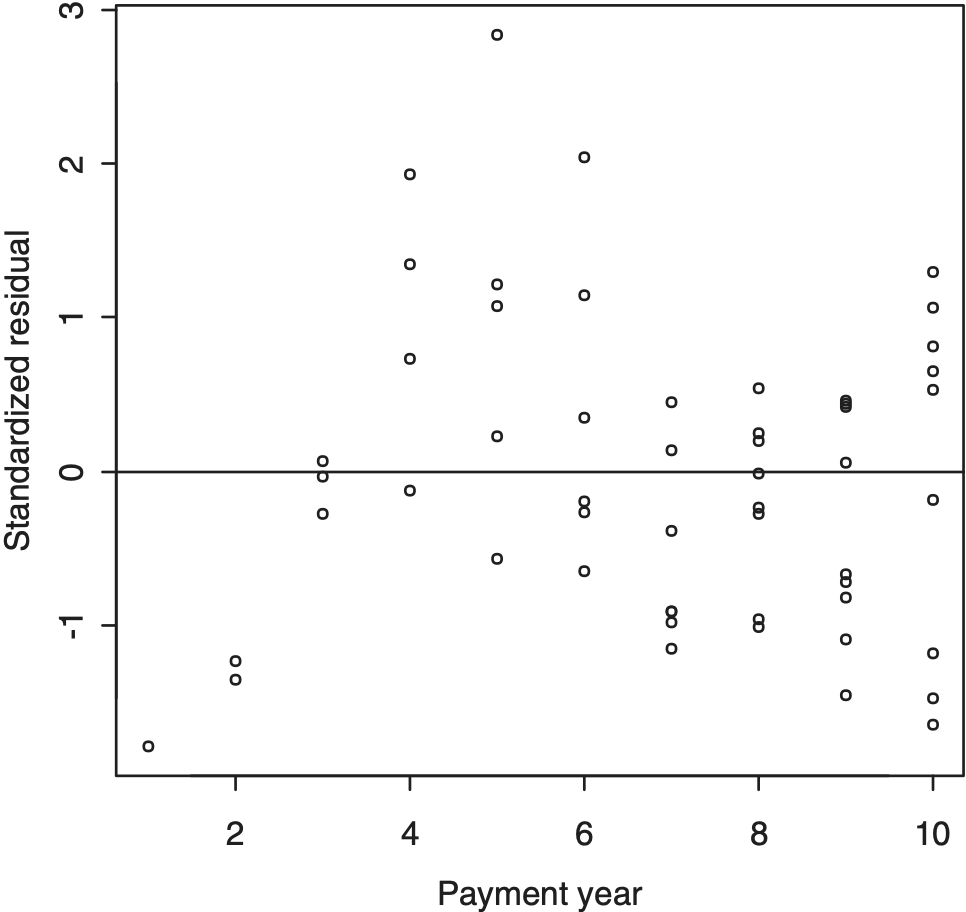
The discussion of weights hitherto has been confined to data anomalies. However, for the PPCF model a more extensive system of weights is required. If weights are set to unity (other than the zero weighting just described), homoscedasticity is not obtained.

This is illustrated in Figure 4.1, which is a plot of standardized deviance residuals of PPCF against OT for Company #1538 (see the data appendix) for which the functions ln λ(.) and ln ψ(.) are quadratic and linear, respectively.

The figure clearly shows the increasing dispersion with increasing OT. This was corrected by assigning cell (k, j) the weight w_kj, defined by

$$\begin{aligned} w_{k j} & =1 \text { if } \bar{t}_{k}(j)<0.92 \\ & =\left\{5+100\left[\bar{t}_{k}(j)-0.92\right]\right\}^{-2} \\ & \quad \text { if } \bar{t}_{k}(j) \geq 0.92 \end{aligned} \tag{4.29}$$

This function exhibits a discontinuity at t̄_k(j) = 0.92 but this is of no consequence as there are no observations in the immediate vicinity of this value of average OT. As seen in Figure 4.1, there is a clump of observation in the vicinity of OT = 0.82 and then none until about OT = 0.92.

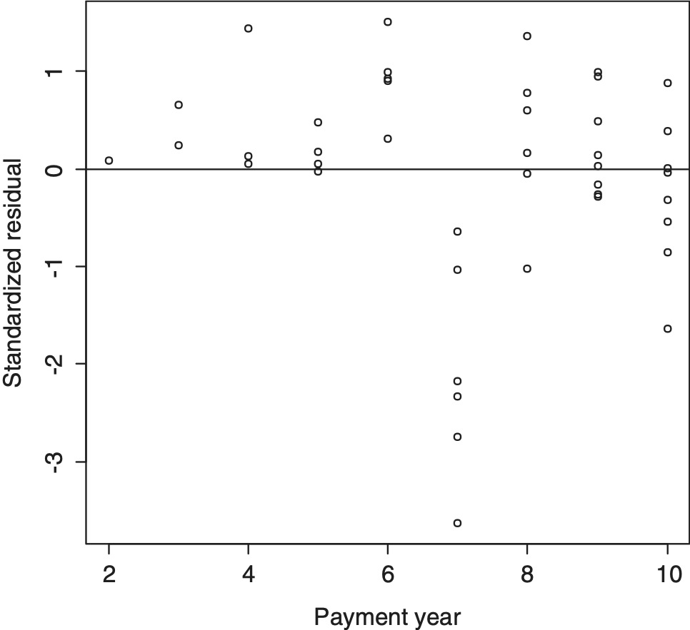
On application of this weighting system, the residual plot in Figure 4.1 was modified to that appearing in Figure 4.2. A reasonable degree of homoscedasticity is seen.

While the weights (4.29) were developed for specifically Company #1538, they were found reasonably efficient for all companies analyzed. They were therefore adopted for all of those companies in the name of a reduced volume of bespoke modeling.

There continue to be few values of average OT in the vicinity of 0.92 when all of the companies analyzed are considered. The discontinuity in (4.29) therefore remains of little consequence. Nonetheless, the PPCF modeling could probably be improved somewhat with the selection of weight systems specific to individual insurers.

Claim closures sub-model

This is characterized by the following assumptions.

1. (FIN1) All cells are stochastically independent, i.e., $F_{k_1 j_1}, F_{k_2 j_2}$ are stochastically independent if $\left(k_1, j_1\right) \neq\left(k_2, j_2\right)$.
2. (FIN2) For each $\mathrm{k}=1,2, \ldots, \mathrm{~K}$ and $\mathrm{j}=2, \ldots, \mathrm{~J}$, suppose that $F_{k j} \sim \operatorname{Bin}\left(U_{k, j-1}+N_{k j}, p_j\right)$, where the $p_j$ are parameters.

This model is evidently an approximation as it yields the result

$$E\left[F_{k j}\right]=\left(U_{k, j-1}+N_{k j}\right) p_{j}$$

which is an overstatement unless all newly reported claims $N_{k j}$ are reported at the very beginning of development year $j$. However, assumption (FIN2) was adopted here because the replacement of $N_{k j}$ by $\kappa N_{k j}$, with $\kappa=1 / 2$ or $1 / 3$, say, generated anomalous cases in which $F_{k j}>U_{k, j-1}+\kappa N_{k j}$.

4.3.3. Calibration

For calibration purposes the PPCF model is expressed in GLM form:

$$Y_{k j} / F_{k j} \sim O D P\left(\mu_{k j}, \phi / w_{k j} F_{k j}^{2}\right) \tag{4.30}$$

where

$$\mu_{k j}=\exp \left(\ln \psi\left(\bar{t}_{k}(j)\right)+\ln \lambda(k+j-1)\right) \tag{4.31}$$

where the function ψ(.) is yet to be determined. This will be discussed in Section 5.3.1.

In the special case of (4.14), the mean (4.31) reduces to

$$\mu_{k j}=\exp \left(\ln \psi\left(\bar{t}_{k}(j)\right)+(j+k-1) \ln \lambda\right) . \tag{4.32}$$

Weights w_kj are as set out in (4.29).

4.3.4. Forecasts

The GLM (4.27) implies the following forecast of Y_kj ∈ 𝔇^c_K:

$$\hat{Y}_{k j}=\hat{F}_{k j} \hat{\alpha}_{k j} \tag{4.33}$$

where

$$\hat{\mu}_{k j}=\exp \left(\ln \hat{\psi}\left(\hat{\bar{t}}_{k}(j)\right)+\ln \hat{\lambda}(k+j-1)\right) \tag{4.34}$$

and ln ψ̂(.), ln λ̂(.) are the GLM estimates of ln ψ(.), ln λ(.) and F̂_kj, t̄̂_k(j) are forecasts of F_kj, t̄_k (j) for the future cell (k, j). As explained in Section 4.2.3, the function ln λ(.) within the GLM will be a linear combination of basis functions, and the estimator ln λ̂(.) is obtained by replacing the coefficients in the linear combination by their GLM estimates. The estimator ln ψ̂(.) is similarly constructed.

Forecasts of future operational times

The forecasts t̄̂_k(j) are calculated, in parallel with (4.23) and (4.26), as

$$\hat{\bar{t}}_{k}(j)=1 / 2\left[\hat{t}_{k}(j-1)+\hat{t}_{k}(j)\right] \tag{4.35}$$

with

$$\hat{t}_{k}(j)=\hat{F}_{k j}^{*} / \hat{N}_{k} \tag{4.36}$$

and the $\hat{F}_{k j}^*$ are, in turn, forecast as

$$\hat{F}_{k j}^{*}=\left(\hat{U}_{k, j-1}+\hat{N}_{k j}\right) \hat{p}_{j} \tag{4.37}$$

where the $\hat{N}_{k j}$ are the same forecasts as in (4.16), the $\hat{U}_{k, j-1}$ are forecast according to the identity

$$\hat{U}_{k j}=\hat{U}_{k, j-1}+\hat{N}_{k j}-\hat{F}_{k j} \tag{4.38}$$

initialized by

$$\hat{U}_{k, j-k+1}=U_{k, j-k+1}(\text { known }) \tag{4.39}$$

and the $\hat{p}_j$ are estimates of the $p_j$ in the GLM defined by (FIN1-2).

This somewhat cavalier treatment of the forecasts F̂_kj is explained by the fact that, provided they are broadly realistic, they have comparatively little effect on the forecast loss reserves R_k. The reason for this is to be found in the concept of OT described in Section 4.3.2.

If expected PPCF is described by a function ψ(t) of OT t, as in (4.28) (disregarding the experience year effect for the moment), then R_k is estimated by

$$\begin{aligned} \hat{R}_{k} & =\hat{N}_{k} \int_{t_{k}(J-k+1)}^{1} \hat{\psi}(t) d t \\ & =\hat{N}_{k}\left(\int_{t_{k}(J-k+1)}^{t_{k}(J-k+2)}+\int_{t_{k}(J-k+2)}^{t_{k}(J-k+3)}+\cdots\right) \hat{\psi}(t) d t . \end{aligned} \tag{4.40}$$

The second representation of $\hat{R}_k$ on the right side expresses it as the sum of its annual components, which depend on the forecasts $\hat{F}_{k j}$. However, the first representation shows that $\hat{R}_k$ depends on only $\hat{\psi}($. and $\hat{N}_k t_k(J-k+1)=\hat{U}_{k, J-k+1}=$ estimated total number of claims remaining unclosed at the end of development year $J-k+1$. There is no dependency on the partition of these $\hat{U}_{k, l-k+1}$ claims by year of claim closure.

The partition of $\hat{U}_{k, J-k+1}$ into its components $\hat{F}_{k j}$ will interact with the experience year effect $\hat{\lambda}(k+j-1)$. If $\hat{\lambda}(.)$ is an increasing function, then the more rapid the closure of the $\hat{\lambda}(k+j-1)$ claims, the smaller the estimate $\hat{R}_k$. However, this is a second order effect and $\hat{R}_k$ is generally relatively insensitive to the partition of $\hat{U}_{k, J-k+1}$ into components $\hat{F}_{k j}$.

4.4. Outlying observations

As pointed out in Section 2.3, the standardized deviance residuals emanating from a valid payments model should be roughly standard normal, most falling within the range (−2, +2).

The residual plots for the models fitted in Section 5.3 do indeed fall mainly within this range. Those of absolute order 3 or more are relatively few but probably of rather greater frequency than justified by the above normal approximation. Those of absolute order 4 or more form a small minority but, again, occur rather more frequently than expected.

The conclusion is that the data set contains some outliers despite the weight correction, but that they are not of extreme magnitude. To have deleted these data points might have created bias. To have attempted any other form of robustification would have opened up the question of how robust reserving should be pursued, a major research initiative in its own right.

Ultimately, with these considerations weighed against the rather mild form of the outliers, no action was taken; the outliers were retained in the data for analysis (unless excluded for some other reason (see Section 5.3)).

4.5. Comparability of different models

4.5.1. Basic comparative setup

The main purpose of the present paper is to compare the predictive power of models that make use of claim closure count data with that of the chain ladder (which does not make use of such data).

The chain ladder, in its bald form, may be reduced to a mechanical algorithm without user judgment or intervention. Objective comparisons that allow for such intervention are difficult because of the subjectivity of the adjustments.

Consequently, the comparisons made in this paper are heavily restricted to quasi-objective model forms. The specific interpretation of this is that, subject to the exceptions noted below:

• All three models (chain ladder, PPCI and PPCF) are applied mechanically in their basic forms as described in Sections 4.1 to 4.3;

• The PPCF function ψ(.) is initially restricted to a simple quadratic form

  $$\ln \psi(\bar{t})=\beta_{1} \bar{t}+\beta_{2} \bar{t}^{2} ; \tag{4.41}$$

• The inflation function λ(.) is restricted to linear (constant inflation rate) or linear spline (piecewise constant inflation rate).

4.5.2. Anomalous accident and experience periods

Occasionally a residual plot will reveal an entire accident or experience year to be inconsistent with others. An example appears in Figure 4.3, which is a plot of standardized deviance residuals against experience year for the unadjusted chain ladder model applied to Company #671.

The anomalous experience of year 7 is evident. In such cases, the omission of that year from the analysis, i.e., assignment of weight zero to all observations in the year, is regarded here as admissible.

On other occasions a residual plot may reveal trending data. If the trend is other than simple, greater predictive power may be achieved by a model that excludes all but the most recent, stationary data than by a model that attempts to fit the trend.

An example appears in Figure 4.4, which is a plot of standardized deviance residuals against experience year for the unadjusted PPCI model with zero inflation, applied to Company #723. The PPCI appear to a positive inflation rate initially, followed by a negative rate, and finally an approximately zero rate. Stationarity appears to be achieved by the exclusion of all experience years other than the most recent 3 or 4.

4.5.3. Experience year (inflationary) effects

Allowances made

As noted in Section 2.4.1, claim payment data are unadjusted for inflation. It is therefore highly likely that they will display trends over experience years. The simple default option for incorporating this in the model is

$$\ln \lambda(s)=\beta s, \tag{4.42}$$

i.e., a constant inflation rate.

The initial versions of the PPCI and PPCF models include the experience year effect (4.42). In some cases, this simple trend is modified to a piecewise linear trend in alternative models.

This default inflationary effect is not incorporated in the chain ladder model for the reason that it would not materially improve the fit of the model to data. The reason for this is well known (Taylor 2000) and is set out in Appendix B.

If a constant inflation rate added to the chain ladder model, it would add one parameter to the model while making little change to the estimated loss reserve. This amounts to overparameterization and the anticipated effect would be a deterioration in the prediction error associated with the loss reserve. This anticipation has been confirmed by numerical experimentation.

In summary, the chain ladder includes an implicit allowance for claim cost escalation at a constant rate. So, the inclusion in the PPCI and PPCF models of claim cost escalation at a constant rate, the rate to be estimated from the data, does not confer any comparative advantage on those models.

As just mentioned, in some cases the PPCI and PPCF models have included a slightly more complex inflation structure than simple linear. This has not been done in the case of the chain ladder, since there is no clear modification of the model that will lead to a data-driven estimate of variations from the constant cost escalation implicitly included in it. For this reason, the differing treatments of inflation in the chain ladder, on the one hand, and the PPCI and PPCF models, on the other, is not viewed as introducing unfairness into the comparison of the different models’ predictive powers.

The inclusion of more complex modeling of experience year effects in the PPCI and PPCF models but not in the chain ladder model simply reflects the greater flexibility of GLM structures over rigid reserving algorithms.

It should perhaps be noted that computations in this paper could equally have been carried out on an “inflation-adjusted basis.” This would involve the adjustment of all paid loss data to constant dollar values and could be applied to all models, including the chain ladder. This is indeed the course followed by Taylor (2000), and such adjustment of the chain ladder can also be found in Hodes, Feldblum, and Blumsohn (1999).

In this case, the inflation adjustment would usually take account of the past claims escalation that “should” have occurred, and within-model estimation would then focus on superimposed inflation, i.e., deviations (positive or negative) of actual escalation from that included in the adjustment.

Extrapolation to future experience years

The chain ladder model contains no explicit allowance for experience year effects, although, as explained above, there is an implicit allowance for a constant inflation rate over the past and extrapolated into the future.

In the case of the PPCI and PPCF models, any allowance for experience year effects will necessarily be explicit. This necessitates decisions about the extrapolations of these effects into future experience years (k + j − 1 > J). The following decision rules have been followed:

• When the past experience year trend takes the constant inflation form (4.42), the same form is extrapolated into the future, i.e., the future inflation rate is assumed constant and equal to the past rate;

• When the past experience year trend takes any other form, it is extrapolated as

  $$\lambda(s)=\lambda(J+k-1) \text { for } s>J+k-1 \text {, } \tag{4.43}$$

i.e., nil future inflation.

4.6. Prediction error

Prediction error has been estimated in conjunction with each loss reserve estimate. This takes the form of an estimate of mean square error of prediction (MSEP) of each R and each of its components R_k. MSEP has been estimated by means of the parametric bootstrap, described in Section 4.6.1.

As noted in Sections 4.2 and 4.3, the PPCI and PPCF models consist of two and three sub-models respectively. These contrast with the chain ladder, which is just a single model.

Each sub-model contains its own prediction error and serves to enlarge the total prediction error in the forecast loss reserve. The allowances made for the contributions of these sub-models are described in Sections 4.6.3 and 4.6.4.

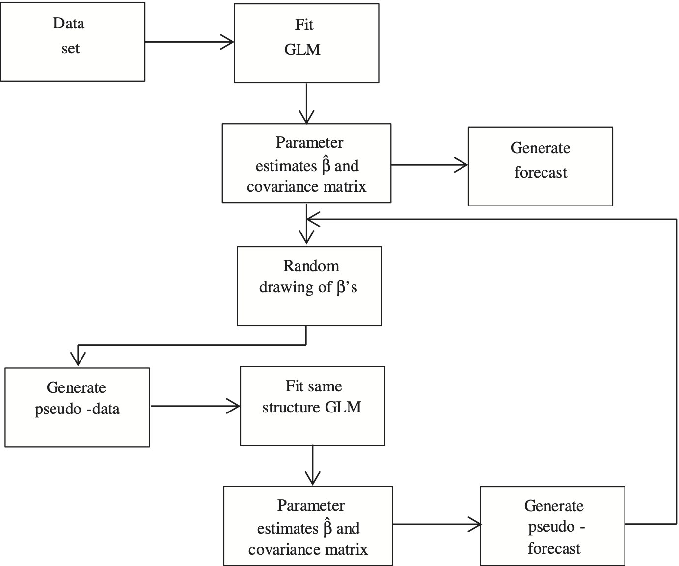
4.6.1. Parametric bootstrap

A parametric bootstrap is used to estimate the distribution of the prediction of any single model. The algorithm for application of this to a GLM is as set out in Figure 4.5.

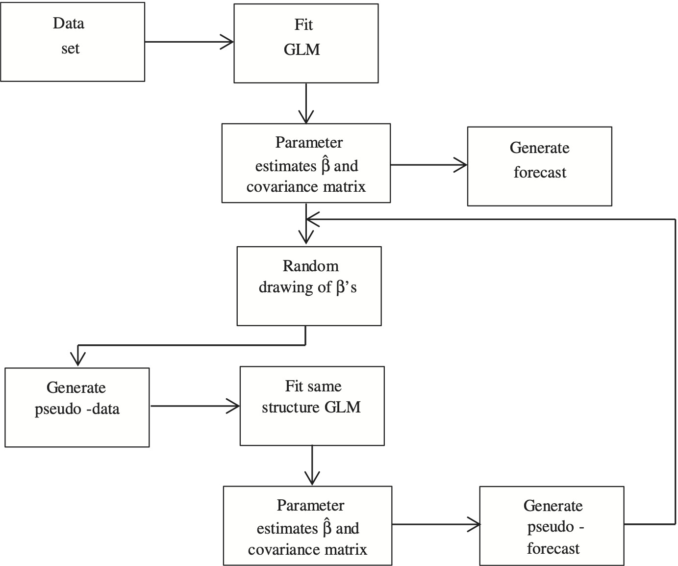
A large sample of pseudo-forecasts, R in number, is generated by this means.

Assume that the GLM takes the form (2.5). The forecast in the figure is

$$\hat{Y}^{f u t}=h^{-1}\left(X \hat{\beta}^{f u t}\right) . \tag{4.44}$$

The randomly drawn vector β, denoted β̃, satisfies

$$\tilde{\beta} \sim N(\hat{\beta}, \operatorname{Cov}(\hat{\beta})) \tag{4.45}$$

where Cov(β̂) is estimated for the GLM. The normality assumption is usually justified by the fact that the estimates β̂ are ML and therefore asymptotically normal with indefinitely increasing sample size.

A pseudo-data set Ỹ is created, consistent with the model form (2.5) and parameter values β̃:

$$\tilde{Y}=h^{-1}(X \tilde{\beta})+\tilde{\varepsilon} \tag{4.46}$$

where $\tilde{\varepsilon}$ is a random drawing of $\varepsilon$, consistent with the error structure assumed for the original GLM and with scale parameter as estimated on the basis of $Y$.

The original model (2.5) is now fitted to $\tilde{Y}$, yielding pseudo-estimates $\hat{\tilde{\beta}}$ and pseudo-forecasts $\hat{\tilde{Y}}^{f u t}$.

By construction, the pseudo-forecasts, denoted $\hat{\tilde{Y}}^{f u r(r)}, r=1,2, \ldots, R$, are iid with the same distribution as $\hat{Y}^{f u t}$. The empirical distribution associated with the sample $\left\{\hat{\tilde{Y}}^{f u r(r)}, r=1,2, \ldots, R\right\}$ is then taken as an approximation to the distribution of $\hat{Y}^{\text {fut }}$.

4.6.2. Chain ladder model

The parametric bootstrap described in Section 4.6.1 is applied to the GLM version of the chain ladder set out in Section 4.1.3.

4.6.3. PPCI model

The PPCI model consists of:

• one GLM for PPCIs, as described in Section 4.2.1, dependent on the N_k; and

• a second GLM to provide forecasts N̂_k of the N_k (Section 4.2.2), which are then used as proxies for the N_k (Section 4.2.3).

Both of these models are bootstrapped and linked according to Figure 4.6.

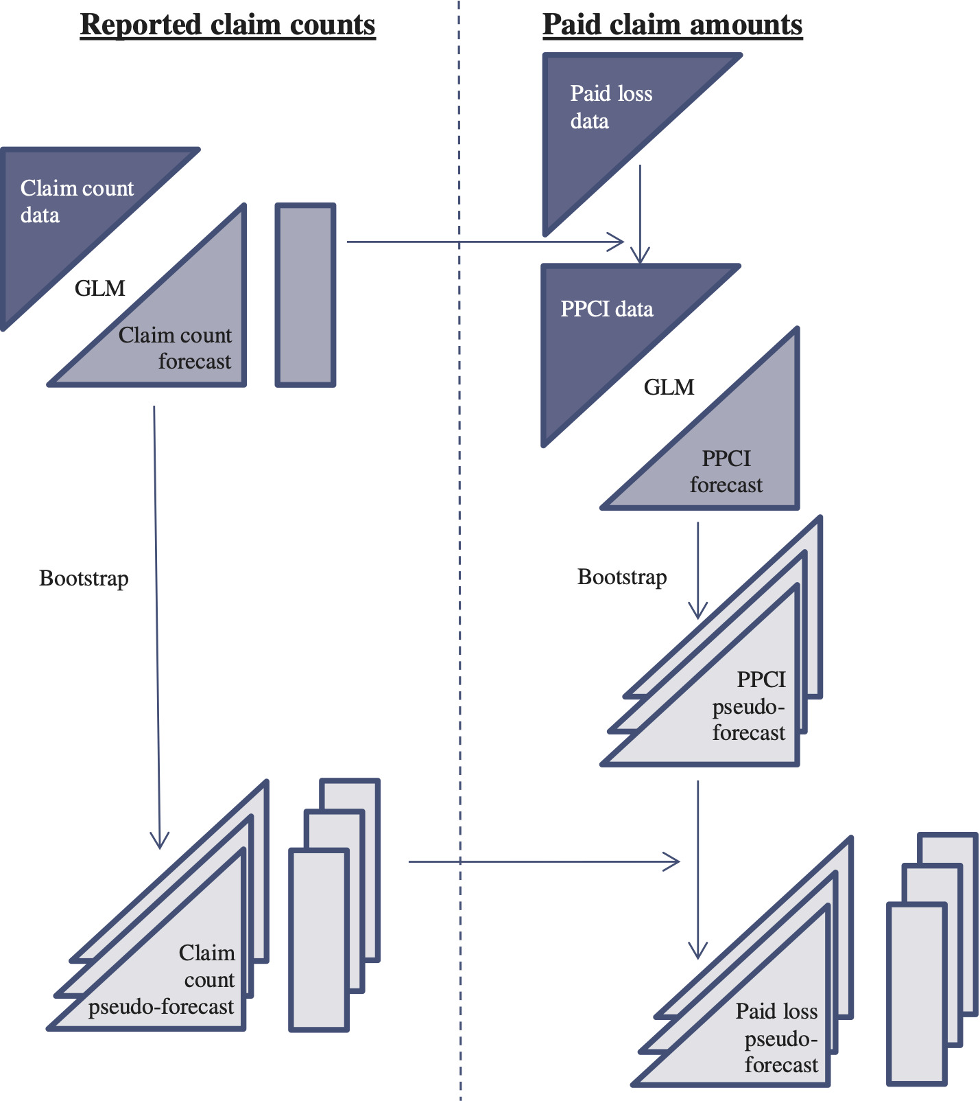
In the figure, input data sets are represented as upper triangles and output forecast arrays as lower triangles. Rectangles represent vectors that consist of row sums of forecast triangles. Thus,

• on the left side of the figure, each entry of the vector represents the forecast number of claims yet to be reported in respect of an accident year;

• on the right side of the figure, each entry of the vector represents the forecast amount of claims yet to be paid in respect of an accident year.

The detail of the bootstrap that appears on each side of the figure is as in Section 4.6.1. Each bundle of triangles is intended to represent the set of pseudo-forecast triangles generated by the bootstrap. Similarly, the bundles of rectangles.

A pseudo-forecast on the left is linked with its counterpart on the right. If in a notation akin to that of Section 4.6.1, $\hat{\tilde{\pi}}_{k j}^{f u t(r)}$ denotes the r-th forecast PPCI for cell $(k, j)$, and $\hat{\tilde{N}}_{k}^{f u t(r)}$ denotes the r-th forecast ultimate number of claims incurred for accident year k, then the r-th forecast of paid losses for cell (k, j) is calculated as $\hat{\tilde{Y}}_{k j}^{f u t(r)}=\hat{\tilde{N}}_k^{f u t(r)} \hat{\tilde{\pi}}_{k j}^{\text {fut }(r)}$.

The final result at the bottom right of the diagram represents the set of pseudo-forecasts $\left\{\hat{\tilde{R}}^{f u t(r)}, r=1\right.$, $2, \ldots, R\}$, where each $\hat{\tilde{R}}^{\text {fut(r)}}$ is a vector of quantities $\hat{\tilde{R}}_k^{fut(r)}$, denoting the $r$-th pseudo-loss-reserve for accident year $k$.

4.6.4. PPCF model

The PPCF model consists of:

• one GLM for PPCFs, dependent on the F_kj, as described in the payments sub-model of Section 4.3.2;

• a second GLM to provide forecasts N̂_k of the N_k (Section 4.2.2), which are then used as proxies for the N_k in the calculation of OTs as in (4.23); and

• a third GLM to provide forecasts of future numbers of claim closures, as described in the claim closures sub-model of Section 4.3.2.

All of these models are bootstrapped and linked according to Figure 4.7, most of which can be interpreted by reference to the description of Figure 4.6. Features peculiar to Figure 4.7 are as follows.

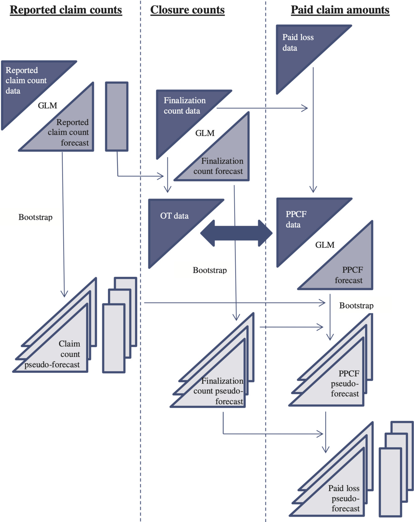
The claim closure counts are seen to be put to two different uses:

• as input to a GLM that forecasts future counts of claim closures; and

• as input to the calculation of OTs.

The OTs just mentioned also require estimates N̂_k as inputs (see (4.23)), and these are obtained as forecasts from a GLM calibrated against the reported claim count triangle, just as in Section 4.6.3.

The block arrow connecting OT and PPCF data is intended to indicate that they form joint input to the GLM of PPCFs.

The figure clearly shows the existence of three separate bootstraps, and the links show how all three contribute to the pseudo-forecasts of PPCFs. Indeed, the pseudo-forecasts of claim closure counts contribute in two distinct ways:

• they lead to pseudo-forecasts of OTs, which are required to form the pseudo-forecasts of PPCFs; and

• they are combined with the pseudo-forecasts of PPCFs to yield pseudo-forecasts of paid losses.

5. Results

5.1. Triangles selected for analysis

Appendix D.1 discusses the LoBs for which claim count data are available and explains why Workers Compensation triangles are selected for this paper’s investigations.

Appendix D.2 discusses the data sets of different companies available within the Workers Compensation LoB, and specific features that might render them unsuitable for inclusion in the following analysis. Ultimately, the data from nine companies is selected for analysis.

The selection relies largely on three formal measures, labeled VRoF1-3, to which reference will be made in the data analysis reported in Section 5.3.

5.2. Model assessment

A major purpose of the compilation of the Meyers and Shi database was the retrospective testing of loss reserve models. Accordingly, one is expected to apply the following procedure to the database or a subset of it:

• Calibrate a model by reference to the training triangle(s), as defined in Section 3.1;

• Forecast loss reserve from the calibration

• Compare forecast with the actual outcomes, as given by the test triangle(s), i.e., symbolically, compare R, as defined by (2.4), with its forecast R̂, and also perhaps compare R_k with R̂_k.

While this approach, applied to a collection of models, will certainly determine which model produced the closest forecasts to subsequent outcomes, this will not necessarily equate to testing the general forecasting qualities of the models.

Strictly, the forecast R̂ should be written R̂⏐𝔇_J, and this should be tested against some value of R that is consistent with 𝔇_J, i.e., one seeks to answer the question “Was R̂ a good forecast on the basis of the information that existed at the end of year J?” Or, expressed another and slightly more precise way, “Was R̂ a tight forecast (small prediction error) under the condition that the state(s) of the world existing over the training interval ℑ_J persist through the test interval?”

If 𝔇^c_J is inconsistent with 𝔇_J, then the difference R − (R̂⏐𝔇_J) will reflect this fact and will not necessarily be informative on the questions just posed. An example will illustrate.

Suppose that wage inflation is consistently 4% per annum throughout the training interval but falls to nil immediately at the end of that interval and remains there throughout the test interval. Suppose this causes the outcome R to be 10% less than would have occurred had the 4% inflation regime endured.

Now consider Models A and B. The former estimates claims inflation to be 4% per annum over ℑ_J. It is sufficiently flexible to be able to produce forecasts on the basis of any desired set of future inflation rates. However, on the basis of 𝔇_J, a future rate of 4% is inserted into it. The resulting forecast is equal to R/0.9. If the future inflation rate had been known from some external source to be nil, the forecast could have been corrected to precisely the correct value.

Model B contains a purely implicit, and non-estimable, allowance for claims inflation. Its forecast is precisely equal to R. It is asserted here that this is not a reasonable estimate on the basis of the facts at the time of its formulation. The same forecast would have remained R had the inflation rate increased rather than decreased. Its equality to its estimand is fortuitous rather than informative.

5.3. Numerical results

5.3.1. Adopted models and results

Table 5.1 lists the company data sets selected for analysis. Each of these has been modeled by chain ladder, PPCI, and PPCF models. In most cases, several variations of each of these models have been tested, and the best in each category selected for comparison with the other categories.

The families of specific model forms are as follows:

Chain ladder model

The model is as set out in (4.5)–(4.7) where weights take the form:

$$\begin{aligned} w_{k, j+1} & =0 \text { if } k+j+2 \in \mathcal{Y}_{C L} \\ & =1 \text { otherwise } \end{aligned} \tag{5.1}$$

with 𝒴_CL ⊂ {1988, . . . , 1997}, a set of experience years specific to the company and model.

PPCI model

The model is as set out in (4.17)–(4.18) where values of the scale parameter take the form (4.20) but with some exceptions, as follows:

$$\begin{aligned} \phi_{k j} & =\infty(\text { cell weight }=0) \text { if } k+j+1 \in \mathcal{Y}_{P P C I} \\ & =\phi \hat{N}_{k}^{2} \text { otherwise } \end{aligned} \tag{5.2}$$

where 𝒴_PPCI ⊆ 𝒴_CL.

While the member of (4.18) involving the function λ(.) was included in a number of test models, in no case did its inclusion produce a model that was materially superior (to that which excluded it). So this member does not feature in the PPCI models summarized in Table 5.2.

PPCF model

The model is as set out in (4.27) where values of the scale parameter take the form:

$$\begin{aligned} \phi_{k j} & =\infty(\text { cell weight }=0) \text { if } k+j+1 \in \mathcal{Y}_{P P C F} \\ & =\phi / w_{k j} \text { otherwise }\left(w_{k j} \text { from }(4.29)\right) \end{aligned} \tag{5.3}$$

where 𝒴_PPCI ⊆ 𝒴_CL, and

$$\psi(t)=\beta_{o T 1} t+\beta_{o T 2} t^{2} \ \mathbf{O R} \tag{5.4}$$

$$\psi(t)=\beta_{O T 1} \ln (1-t)+\beta_{O T 2}[\ln (1-t)]^{2} \ \mathbf{O R} \tag{5.5}$$

$$\psi(t)=\beta_{O T 1}(1-t)^{0.35}+\beta_{O T 2} \min (0.8, t) \tag{5.6}$$

$$\ln \lambda(i)=\sum_{h=1}^{H} \beta_{Y h} \max \left(0, \min \left(y_{h}, i-y_{h-1}\right)\right) \tag{5.7}$$

for a defined set of values $\left\{y_0, \ldots, y_H\right\}$ subject to $y_0=1988, y_H=1997$. Some coefficients $\beta_{Y h}$ were set to zero before model fitting commenced.

Equation (5.7) represents the experience year effect as a linear spline with $H-1$ knots $\left\{y_1, \ldots\right.$, $\left.y_{H-1}\right\}$. The gradient of the spline segment over the interval $i \in\left(y_{h-1}, y_h\right)$ is $\beta_{Y h}$. The following special cases occur:

1. H = 1: (5.7) reduces to a simple linear function over the interval i ∈ (1988,1997) (constant rate of claim cost escalation, as in (4.14)).

2. H = 0: By convention, (5.7) is taken to be null.

Table 5.1 sets out the specific model choices adopted and whose results are reported in Table 5.2.

Table 5.2 displays the principal results obtained from the application of the models described in Table 5.1. Detail underlying the table appears in Appendix C.

The left part of the table reports the “CoV” or coefficient of variation of the forecast loss reserve, defined as:

$$\text { CoV }=\frac{\text { MSEP }^{1 / 2}}{\text { Forecast loss reserve }} \tag{5.8}$$

where both numerator and denominator are obtained from the bootstrapped empirical distribution of outstanding losses described in Section 4.6.1.

The right part of the table reports the ratio of forecast loss reserve to the actual claim cost outcome from the test triangle.

For each company in Table 5.2, the smallest CoV(s) are displayed in bold italic font. The associated model(s) are the “winner(s)” for that company. Table 5.3 records the score of each model, where the score is equal to the number of wins out of the nine cases, with a score of ½ in the case of a two-way tie and a score of ⅓ in the case of a three-way tie.

It is seen that the use of count data equals or improves prediction error in 7.1 cases out of nine, i.e., 80% of the cases, and positively improves it in six cases out of nine (67%). The extent of the improvement is shown in Table 5.2.

5.3.2. Discussion of results

It is instructive to examine the circumstances in which the different models produce superior predictive performance. This may be done by examining Table 5.3 and Table 5.2 in conjunction.

Company #3360

The chain ladder is the clear winner in only one case, namely, company #3360. VRoF1 and VRoF2 in Table D.3 in Appendix D.2 indicate that this portfolio is characterized by extremely variable rates of claim closure. The details of this appear in Table 5.4, which displays the company’s triangle of OTs (actually complements thereof).

If rates of claim closure had been constant, then entries in this table would have been constant within each column. Evidently, this is far from the case.

A number of cells are shaded in Table 5.4, indicating likely disruptions to, or errors in, the data.

• Accident year 1988. There is no entry for development year 1. This is because no claims were reported for this cell, rendering calculation of numbers of claim closures impossible. It appears that the number of claims reported as received in development year 2 was actually the total for development years 1 and 2.

• Accident year 1990. The entries for development years 5 and 6 indicate that cumulative numbers of claim closures to those years exceeded the total number of claims estimated as incurred (N̂_k) for 1990, which in turn exceeds the total number reported to the end of the relevant development year. This indicates the presence of data errors. Examination of the source data enables this anomaly to be traced to a large and negative number of claims reported in development year 6 (see Appendix A.2.6).

• Accident year 1996. This year is subject to dramatic increase in the rate of claim closure over accident year 1995, and one that is not sustained into accident year 1997. Reference once again to the source data for reported claims in Appendix A.2.6 reveals a dramatic increase in claim counts in accident year 1996, followed by a reversal of this in accident year 1997. Net earned premium did not change markedly over this period. To all appearances, either:

  1. the data for the accident year are erroneous; or

  2. the nature of the claims incurred changed abruptly, and temporarily, around 1996.

It is evident that the reliability of the models depending on claim counts (PPCI and PPCF) will be a function of the reliability of those counts. In the present case, there is clear evidence of errors in the counts and other cause to view them with suspicion.

In the case of clearly erroneous data (Appendices A.2.6 and A.3.6), the offending cells have been assigned zero weight in any modeling. However, it is possible (probable?) that adjacent cells at least carry similar anomalies that are not manifestly errors, e.g., quantities (1-OT) are understated but not actually negative.

The conclusion of this reasoning is that the application of PPCI and PPCF models to company #3360 was dubious from the start, and it is perhaps not surprising that the chain ladder forecast appears superior. One might observe at this point that, although models dependent on claim counts, such as PPCI and PPCF, can lead to improved predictive power, relative to models independent of these counts, they require reliable counts, and so can be more sensitive to data irregularities.

Company #1694

For this company the chain ladder is involved in a two-way tie, with the PPCI model as the best predictor.

Reference to Table D.3 indicates little overall variation in rates of claim closure (VRoF1), and OTs at the end of 1997 reasonably close to average values (VRoF3), though some appreciable movement in OTs observed in development year 1 (VRoF2). The detail appears in Table 5.5.

The single large shift in OTs occurs in development year 1 in the transition from accident year 1989 to 1990. One may conclude then that the claim closure count data adds little information. In this case it is unsurprising that PPCF model is outperformed by the other two.

Company #4731

For this company the chain ladder is involved in a three-way tie with the PPCI and PPCF models as the best predictor.

It is noted in the commentary following Table D.3 that this company appeared to have experienced relatively stable rates of claim closure by all three criteria VRoF1-3. However, reference was also made to the fact that some of the ratios in d(j)/m(j) in VRoF1 were material. Specifically, these were development years 6, 7 and 8. The individual development year contributions to VRoF1 were as shown in Table 5.6.

The instability of rates of claim closure in development years 6 and later suggests that the PPCF model may produce loss reserve forecasts of superior reliability in accident years whose liability relates mainly to these development years.

Table 5.7 gives the CoVs of loss reserve separately by accident year for each of the three models. The loss reserve for accident year 1989 and 1990 do not involve development years 6 to 8, only 9 and 10. The PPCF model is not superior here.

On the other hand, loss reserves for accident years 1991 to 1993 are dominated by development years 6 to 8, and accident year 1994 is heavily affected by them. And here the PPCF model does produce superior performance.

The influence of these development years steadily diminishes with accident year increasing from 1994. And, sure enough, the PPCF model loses it superiority in these accident years.

Company #1538

Table D.3 shows this company to have exhibited a consistently high degree of variation in rates of claim closure. The detail appears in Table 5.8.

Thus, company #1538 appears a priori to be a good candidate application of the PPCF model. And so it proves in Table 5.2, where that model outperforms its two rivals and, in particular, outperforms the chain ladder by a large margin.

It may be noted that there is some uncertainty concerning the numbers of claims incurred, and hence the OTs, for the company due to the high error rate in the triangle of numbers of claims reported (Appendix A.2.3).

Company #38733

Table D.3 also indicates a consistently high degree of variation in rates of claim closure of this company. In an apparent paradox, however, the PPCF model performs extremely poorly.

Part or all of the explanation in this case appears to lie in faulty data. The triangle of claim closure counts appears in Table 5.9, in which anomalous observations have been shaded.

The entry of 282 in accident year 1989, development year 8 appears most peculiar and seems likely to be a misstatement. It arises from a recorded number of 281 claims reported in the cell, whereas the expected number would have been 1 or 2. In addition, there are systematic anomalies in accident years 1988 and 1989. One may be forgiven for considering these data of dubious integrity.

A version of the PPCF model was produced in which all observations associated with either or both of accident year 1989 and experience year 1993 were assigned zero weight but without improvement in prediction error. The reason for this may be as follows.

If there were data errors in the shaded cells, there might be sympathetic errors in other cells. For example, claim closure counts in experience year 1993 appear low for a number of accident years. If this derives from some systematic misreporting whereby some claim closures from that experience year have been assigned to others, then a large number of entries in the table may be incorrect.

All in all, it is difficult to assess the quality of claim closure count data for this company and the applicability of the PPCF model.

6. Model extensions

It is explained in Section 4.5.1 that, for comparability with the chain ladder model, the PPCI and PPCF models are restricted to relatively simple and mechanical forms. No attempt has been made to optimize these model forms. It is likely that further investigation would lead to improved model forms, with accompanying reduction in their respective prediction errors.

6.1. PPCI model

Some simple possibilities can be outlined. First, recall assumption (PPCI2) in Section 4.2.1, leading to (4.13). According to this, the expected PPCI in cell $(k, j)$ takes the form $\pi_j \lambda(k+j-1)$. The development year effect $\pi_j$ is treated here as a categorical variable, and so estimates are required of the 10 parameters $\pi_1, \ldots, \pi_{10}$.

This is done for comparability with the chain ladder model, which similarly specifies age-to-age factors as the categorical variable $\ln g_j$ in (4.6). It represents, however, parametric profligacy, as it is likely that some parametric form $\pi(j)$ could be found that would represent the development year effect almost as accurately as $\pi_j$ and with considerably fewer parameters. This would reduce prediction error.

For example, Hoerl curves, as used by De Jong and Zehnwirth (1983), are sometimes used to represent the development year effect. These take the gamma-like parametric form:

$$\ln \pi(j)=\beta_{1} \ln j+\beta_{2} j \tag{6.1}$$

represented by just two parameters instead of 10.

6.2. PPCF model

One of the distinctions between the PPCI and PPCF models is that the latter contains an OT effect that is already expressed parametric form (see (5.4) to (5.6)). However, one of the requirements of the model in Section 4.5.1 is that initially ψ(.) take the same form for all insurers.

This restriction is relaxed later, but it is still fair to say that the parametric form of ψ(.) has been only lightly researched. Further investigation might lead to improved prediction error of the PPCF model.

6.3. Hybrid forecasts

Table 5.7 raises the possibility of hybrid forecasts. For example, one might base the loss reserve on, say:

• the PPCF model for the middle accident years 1991–1995; and

• the PPCI model for the early and late accident years 1989–1990 and 1996–1997.

The effect is close to optimization of the CoV of the total loss reserve. This would be less than the CoV from any one of the models. Note that this diversification from a single model is likely to reduce correlation across accident years, which will also contribute to reduction in the CoV of the total loss reserve.

Hybrid forecasts are discussed further in Chapter 12 of Taylor (2000).

6.4. Incurred losses

This paper has concentrated on incremental paid claim data, its analysis, and subsequent forecast. The same data source also provided triangles of incurred claims (defined in a cell as equal to paid claims adjusted by the increase in case estimates of unpaid claims over the interval from beginning to end of the cell).

The incurred claims data has not been used here. However, it could have been subjected to analysis by means of the chain ladder and other models. Those other models would not have been PPCI or PPCF but would need to have been adapted to case estimate data. Some of the issues associated with such models are aired in Section 4.4 of Taylor (2000).

How the chain ladder would have fared in competition with these other models remains to be seen. This exercise is left for other investigators.

7. Conclusion

The purpose of the present paper has been to test whether loss reserving models that rely on claim count data can produce better forecasts than the chain ladder model (which does not rely on counts)— better in the sense of being subject to a lesser prediction error.

A couple of commonly cited arguments against the use of count data have been canvassed in Section 1. It is suggested here that the data be allowed to speak for themselves, and that count data be used if doing so reduces prediction error, and not used otherwise.

Section 1 discussed the fact that the mechanistic form of chain ladder applied in the numerical investigations of Section 5 will not always align with the subjective adaptations of the model that are found in practice, and considered whether this would confer an unwarranted disadvantage on the chain ladder. To be sure, there is some force in this argument.

However, there are some countervailing considerations that deserve note. The GLM formulations of the competing formal models (PPCI and PPCF) are inherently flexible, and this is a strength of each. Since the chain ladder has been applied as a largely mechanical algorithm without user judgement or intervention, the competing models have also been largely constrained to relatively mechanistic versions. In this sense, all models have been hobbled to some degree in the comparisons, though whether equally hobbled is an open question.

Section 1 also noted a lack of methodology for the estimation of the prediction error associated with a subjective model. Prediction error is estimated by bootstrapping in the present paper and, while the application of a bootstrap to a subjective model would be technically possible, its results might well be misleading for the following reason.

The parametric bootstrap described in Section 4.6.1 cannot be applied to a model that is a fully defined stochastic model, but a nonparametric bootstrap (Shibata 1997), which depends on only the differences between actual and model age-to-age factors, would be possible.

This form of bootstrap would involve the construction of pseudo-data sets from those residuals, but the features of the pseudo-data sets would be likely to differ from the features of the original data set in such a way that the subjective adjustments selected in relation to the original data set would likely be incompatible with some of the pseudo-data sets. In such circumstances, the bootstrap results might be difficult to interpret, or even meaningless.

The question at issue has been tested empirically by reference to the Meyers-Shi data set. While this includes data from a large number of portfolios, many of these are unsuitable for various reasons.

Ultimately the empirical investigation relies on only nine workers compensation portfolios. This is limited, and it is unlikely that the results can be considered conclusive. On the other hand, a consistent and coherent narrative emerges from the results, in the sense set out in the findings below, and to the point where the results may be considered at least compelling.

The nine selected data sets were chosen according to a number of criteria (detail in Section 5.1), including material changes in rate of claim closure over the training interval. These are the circumstances in which the PPCF model in particular is, on a priori considerations, likely to perform well for, in the event of claim closure rates that remained strictly constant over time, claim closure counts would add no information to the loss process and forecast based on them would be expected to be inferior.

The first finding is that, for the selected data sets, the success of the chain ladder is limited. Either PPCI or PPCF model produces, or both produce, at least equal performance, in terms of prediction error, 80% of the time, and positively superior performance two-thirds of the time (Section 5.3.2).

When the chain ladder produces the best performance of the three models, the reasons are evident. Either count data contain erratic entries (companies #3360, #38733), or rates of claim closure are less variable than at first appeared (company #1694).

The first case is one in which the data speak for themselves; the second is a demonstration of the conclusion already reached that the chain ladder is likely to produce reliable estimates, relative to the PPCF model at least, in the presence of a high degree of stability in rates of claim closure.

For a portfolio characterized by consistently high variation in claim closure rates (company #1538), the PPCF model is likely to produce the forecast of loss reserve that has the lowest prediction error.

Sometimes variation in claim closure rates is seen to affect some accident years particularly and others less so (company #4731). In these cases it is likely that the PPCF model will produce superior forecasts for the accident years affected and inferior forecasts for the others.

As noted at the end of Section 1, the methodological qualifications set out above on the model comparisons render those comparisons less than definitive. However, as far as they go, they lead to the conclusion that, in certain (reasonably predictable) circumstances, the reliance on claim count information in forecasting loss experience improves the forecasts.

The major uncertainty relates to whether certain subjective, and therefore not well defined, adjustments to models that do not rely on claim counts might be sufficiently judicious as to reverse this paper’s main finding. Demonstration of a proposition of this sort would be inherently difficult. It would require demonstration of the superiority of an undefined model according to an undefinable criterion of superiority.

In any event, if the authors are to reveal their colors, they would view such a proposition as extremely dubious. The effects on age-to-age factors of changing closure rates, diagonal effects, and other perturbations of the claims triangle, and especially combinations of these, can be subtle and the success of subjective adjustments for them limited.

One would be entitled to ask why subjective allowance for disturbances to a formal model would be superior to formal modeling, and what aspect of subjective adjustment is not achievable within a formal model. Cannot all the subjective adjustments be objectified?

Of the three LoBs for which count data were available, two (Private Passenger Auto and Commercial Auto) were short tailed. Here the more limited reserving challenge suggests that models of simple form, such as the chain ladder, might be the order of the day and that more elaborate models might add little, if anything.

The remaining LoB, on which the present study has relied, is only medium tailed, relative to some other Liability LoBs (e.g., Auto Bodily Injury, Public Liability). Typical experience is that the advantage of PPCI, and particularly PPCF, models over the chain ladder increases with tail length, since the longer-tailed LoBs bring rates of claim closure more into play.

Moreover, the PPCF model is best adapted to claims whose payments are concentrated close to the claim closure date. This is typical of claims subject to settlement under the law of tort. The long-tailed LoBs cited above satisfy the condition but the workers compensation LoB usually would not.

From this follows an expectation that the conclusions reached in this paper in connection with the workers compensation LoB would be likely to emerge in starker relief if a long-tailed LoB were investigated (see, e.g., Taylor 2000; Taylor and McGuire 2004).

Acknowledgments

This paper was prepared with the benefit of partial research funding from the Actuaries Institute of Australia and also from Taylor Fry Consulting Actuaries.

We wish to express our gratitude to Dr. Peng Shi who privately made available the triangles of count data exemplified in Appendices A.2 and A.3.