Applying Graphical Models to Automobile Insurance Data

1. Introduction

In a data-driven decision-making environment, analysis of insurance data provides input for making decisions regarding underwriting, pricing of insurance products, claims and profitability. The focus of this paper is to study the dependency structure of categorical variables pertaining to the Australian automobile insurance data and to explore potential applications to determination of frequency rates by rating classes.

Insurers gather information about their policy holders at the time of writing insurance policies. The data collected by an insurance carrier depends on the line of business offered, business expediency, and legal constraints. The rating variables are used to price insurance products based on the insured’s characteristics and are helpful regarding underwriting selection. Rating variables are of mixed measurement types. Our focus here is only with respect to the categorical variables used in the Australian Automobile insurance data.

The analysis of insurance data is a multifaceted endeavor. The goals of statistical data analysis are broadly of two types: understanding and prediction. Understanding encompasses summarization as well as inference.

Tasks associated with machine learning, i.e., learning from data, are categorized as supervised learning and unsupervised learning. Predictive modeling is an example of supervised learning, where features are used to predict the value of a target variable.

Unsupervised learning is mainly concerned with finding relationships between features, or grouping of instances as to reveal hidden underlying structure of data with no designated target variable involved.

The goal of the analysis in this paper is primarily about understanding and an exercise in unsupervised learning.

We consider exploratory data analysis (EDA) tools suitable for categorical variables. Inferential procedures such as tests of independence and fitting log-linear models to data are discussed. Furthermore, we discuss some limitations of these tools and procedures.

We now proceed with briefly outlining the contents of the other sections. Description of the data used and exploratory data analysis, as well as preprocessing of the data, are covered in section 2. In section 3, we consider two-way contingency tables, using the Pearson chi-square test for assessing the strength of association between two categorical variables. Mosaic plots, as a visualization tool, are used to present two-way contingency tables, and we discuss some limitations of analysis based solely on two variables. Section 4 considers the analysis of three categorical variables. In particular, we extend the description of mosaic plots to that of three variables, introduce log-linear models, the concept of conditional independence, and graphical modeling. Considerations of more than three categorical variables and model selection have been relegated to section 5. The use of graphical modeling for exploring dependency structure of categorical variables, potential applications to determining frequency rates, and overfitting are also discussed in section 5. Summary and concluding remarks are stated in section 6.

An attempt has been made to blend theory with the necessary statistical computations, so that the paper will be useful to practicing actuaries.

2. Data and data preprocessing

Insurance data are generally propriety information of the insurance companies and are not publicly available. The data used in this paper is available from the following website and has been referenced in the book co-authored by De Jong and Heller (2008): http://www.businessandeconomics.mq.edu.au/our_departments/Applied_Finance_and_Actuarial_Studies/research/books/GLMsforInsuranceData/data_sets.

The data consists of one year of Australian vehicle insurance policies taken out in 2004 or 2005. The name of the data set is car.csv and there is a brief description of the variables considered in the file named vehicle.txt which has been reproduced here in the Appendix A.1. There were 67,856 observations, and for each record the values of ten attributes were given.

The software R has been used to perform computations and display graphics. R is an open-source software useful for doing statistical analysis and data visualization. The base package of R has many useful standard functions, and there are over 4,000 supplemental packages which enhance the capabilities of R. Information about R and its associated packages can be obtained from http://cran.r-project.org/. Some of the R functions used in this paper are referenced in Appendix A.2 and may be of interest to practicing actuaries.

A quick “feel” of the data can be obtained from Exhibit 2.1 and Exhibit 2.2.

Exhibit 2.1 provides information about the name, type of measurement, and sample values for each variable in the automobile data set. For instance, Vehicle Value (veh_value) is a continuous (num) variable with sample values in unit of 10,000 while Vehicle Body Type (veh_body) is a nominal attribute.

Exhibit 2.2 provides crude information regarding (a) whether a variable is symmetrically distributed, (b) appearance of outliers, and (c) if there are any inconsistent observed values.

The analysis in this paper is primarily concerned with the categorical—nominal or ordinal—attributes. The preprocessing of the data involved: (a) change of names of the variables used for easier references, (b) transformations of two of the variables, and (c) selecting seven out of the ten variables for this study. Additional details are provided in Appendix A.3.

The variable “Value” was originally recorded on a numeric scale. Value is used as a proxy for “size” and or “power” of a vehicle and serves as an underwriting variable. Since our primary interest is with categorical variables, it was decided to include Value in our analysis as an ordinal rather than numeric variable. The process of transforming a numeric variable to an ordinal variable is referred to as binning or feature-discretization; see Kantardzic (2011). There are two commonly used methods for binning. One method uses equal frequency and the other uses equal length. Here, we chose the equal frequency approach. The 25% quartile (1.01), 50% quartile (1.50) and 75% quartile (2.15) of the Value were selected as cutoff points for binning.

The other transformed variable was the “Body.” The categorical variable Body had originally thirteen levels. Some of the levels had relatively low frequencies (see Table 2.1). These low frequency classes can affect the results of some statistical procedures used to fitting a model to the data. Reducing the number of levels, i.e., collapsing, may be achieved subjectively based upon an expert’s opinion, or it may be determined objectively based on a certain criterion. I decided to consider the variable Claim in conjunction with Body to reduce the number of levels to be used; see Table 2.1.

For any two levels of the Body type, we can measure their “closeness” by using the Euclidean distance based on the relative frequencies. For instance, to see how close is “BUS” to “CONVT,” the Euclidean distance is computed as follows:

$$\begin{array}{l} d(B U S, \text { CONVT }) \\ \quad=\sqrt{(0.00062-.00123)^{2}+(0.00195-0.00065)^{2}} \\ \quad=0.00144 \end{array}$$

The distance between any two distinct levels of the Body has been computed and organized as a distance matrix in Exhibit 2.3.

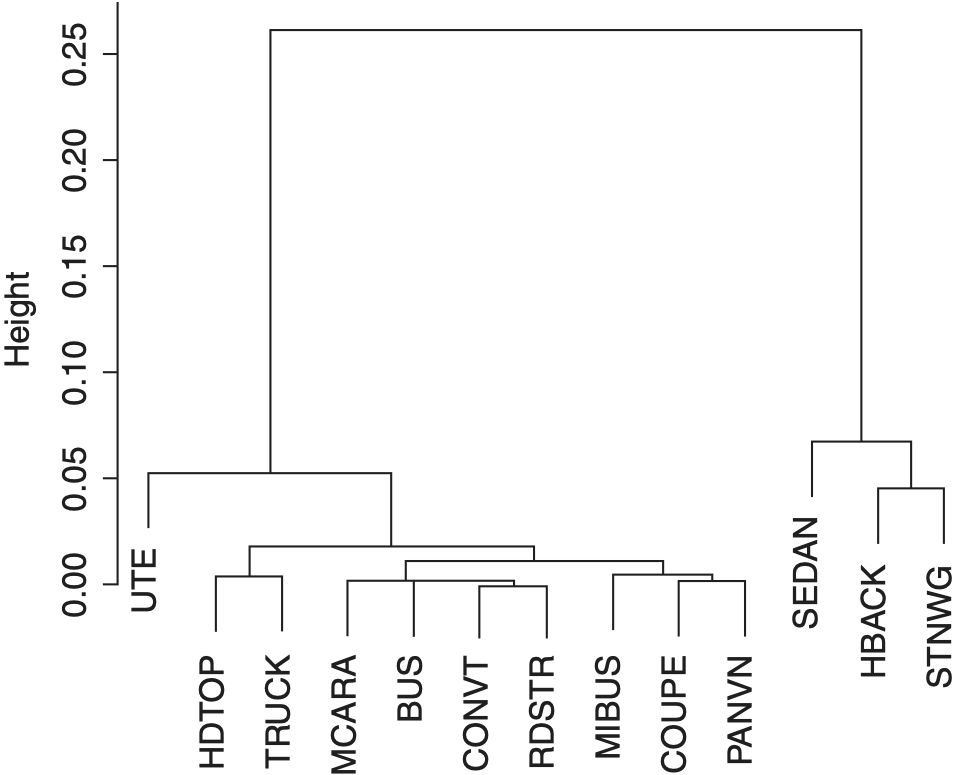
The matrix of distances is used as an input to a hierarchical clustering algorithm for grouping levels of the Body. For an explanation of the hierarchical clustering method, refer to Johnson and Wichern (2007). The output of the hierarchical analysis is a dendrogram (an inverted tree); see Exhibit 2.4. The lower section of the dendrogram suggests combining the low frequency levels BUS, CONVT, MCARA and RDSTR into a single class labeled “Other.” Hence, the number of levels of Body was reduced from thirteen to ten. Furthermore, the label of the levels was changed from character to numeric type to facilitate graphical presentation.

Exhibit 2.4.Dendrogram

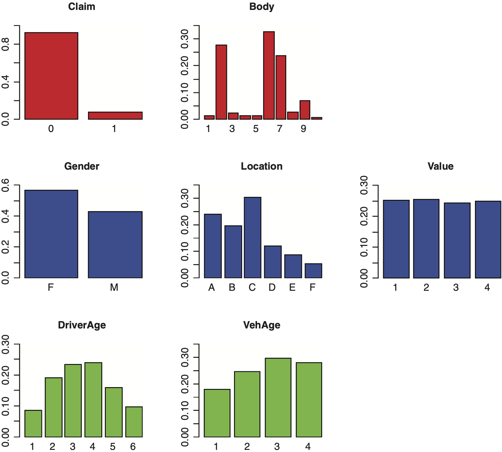
Bar charts are commonly used to show the frequency distributions of categorical variables. In Exhibit 2.5, we display the bar charts for the attributes studied here, based on their relative frequencies.

Now, we may proceed with the statistical analysis phase of the paper.

Exhibit 2.5.Bar charts for relative frequency of attributes studied

3. Analysis of two categorical variables

In this section, we discuss exploratory tools as well as a statistical test of independence for two categorical variables. The information about two categorical variables is summarized as a two-way contingency table obtained by cross-tabulating the data. The contingency table for Value and Vehicle Age is given by Table 3.1. The top-left panel of Exhibit 3.1, a mosaic plot, provides a graphical display corresponding to the contingency Table 3.1.

Exhibit 3.1.Mosaic plots for Value and Vehicle Age as well as Claim and Gender

The association between two categorical variables is determined by conducting a Pearson chi-square test of independence.

Let us proceed with introducing the necessary notations and terms needed to perform the Pearson chi-square test.

For two categorical variables A and B, having domains dom(A) = {1, 2, . . . , J} and dom(B) = {1, 2, . . . , K}, the subset of the data with A = j and B = k is labeled as the cell (j, k) ∈ dom(A) × dom(B). A two-way cross-tabulation of the data determines all cell frequencies, n_jk’s. The Pearson chi-square test statistic, X² , is defined as

$$X^{2}=\sum_{j=1}^{J} \sum_{k=1}^{K} \frac{\left(n_{j k}-\hat{m}_{j k}^{(0)}\right)^{2}}{\hat{m}_{j k}^{(0)}}$$

where n_jk is the observed frequency count for the cell (j, k); m̂_jk⁽⁰⁾, the expected count for the cell (j, k), assuming the validity of independence hypothesis for A and B. That is, $\hat{m}_{j k}^{(0)}=\frac{n_{j+} n_{+k}}{n}$; where n_j+ and n_+k are the jth row total and kth column total, respectively, of the two-way contingency table, and n denotes the total number of observations.

Based on the validity of the null hypothesis of independence, the statistic X² is asymptotically distributed as a chi-squared random variable with (J − 1) (K − 1) degrees of freedom. Large observed values of X² or alternatively small p-values do not support the null hypothesis of independence. A chosen p − value = α ≤ 0.05 leads to rejection of independence hypothesis where α is the significance level of the test; see Christensen (1997).

Our analysis of the Australian Automobile data involved seven categorical variables. Twenty-one Pearson chi-square tests of independence were performed. It is interesting to note that only in the case of Claim and Gender, we failed to reject the null hypothesis of independence.

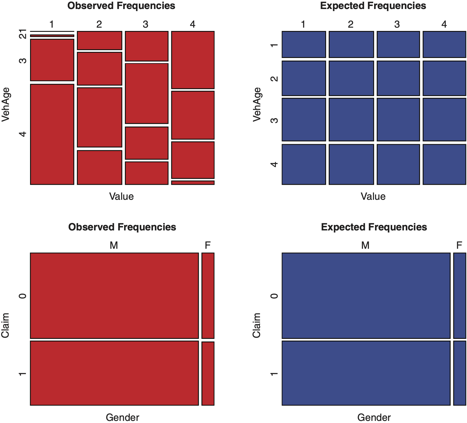
A mosaic plot (see top left panel of Exhibit 3.1) provides a graphical display corresponding to a two-way contingency table. The methodology to construct mosaic plots has been explained by Friendly (1994). A mosaic is composed of tiles, where each tile corresponds to a cell of a contingency table. To the cell (j, k), 1 ≤ j ≤ J, 1 ≤ k ≤ K, there corresponds a tile labeled (j, k) whose width is proportional to n_+k and its height is proportional to $n_{j \mid k}=\frac{n_{j k}}{n_{+k}}$, the conditional count; see top left panel of Exhibit 3.1, where J = K = 4. The area of the (j, k) tile is proportional to the cell frequency n_jk.

Under the independence assumption, the expected frequency for the cell (j, k) is $\hat{m}_{j k}^{(0)}=\frac{n_{j+} n_{+k}}{n}$. Hence, the height of the (j, k) tile is proportional to n_j+ which does not depend upon k, the second variable. Based on the independence assumption, for each j (horizontal level, representing the first variable), tiles in the jth row with differing k values have the same height; see the top right panel of Exhibit 3.1.

The mosaics corresponding to observed and expected frequencies for categorical variables Value and Vehicle Age, shown in Exhibit 3.1, top left and top right, are dissimilar. This lack of similarity is consistent with rejection of the chi-square test. On the other hand, the mosaics in the bottom right and bottom left of Exhibit 3.1 appear similar, and this outcome is consistent with failing to reject the independence test for Claim and Gender.

Furthermore, one notices the anomaly between observed and expected frequencies for the cell corresponding to the Value of 1 and Vehicle Age of 4 in Exhibit 3.1. Hence, mosaic plots reveal further information beyond independence.

There are some limitations to relying only on two categorical variables. First, if there are more than two categorical variables available, then it seems logical to use all the available variables, as more information tends to lead to better decisions. Second, when there are other categorical variables available, say, three in total, then, in some instances, the inferences based on two categorical variables, a marginal approach, may contradict the conclusion based on using all three. These anomalies are referred to as Simpson’s paradox; see Agresti (2002).

4. Log-linear models, conditional independence, and graphical modeling

In this section we consider log-linear models, three-way mosaic plots, the concept of conditional independence, and graphical models as they relate to three categorical variables.

To perform a test of independence involving three categorical variables, one approach is to extend the Pearson chi-square test to the case of three factors. Alternatively, a preferred approach is to use the log-linear models.

Log-linear models are a special class of the generalized linear models, GLM, which extend the classical regression models. In classical regression analysis, the mean of a continuous response variable is related to a set of explanatory variables, assuming that the response variable is normally distributed. With log-linear models, one relates the expected cell count of a multidimensional contingency table to a set of categorical variables by specifying their main and interaction effects. This approach mirrors the ANOVA procedure where a continuous response variable is related to a set of explanatory factors. An advantage of using the log-linear approach over the Pearson chi-square test is that it allows for testing alternative dependency structure among the categorical variables. Useful references for log-linear models are Agresti (2002), Fienberg (1980) and Christensen (1997).

We begin by describing log-linear models for two categorical variables A and B, although our focus is with more than two variables.

Let A and B have respective domains dom(A) = {1, 2, . . . , J} and dom(B) = {1, 2, . . . , K}. For the cell (j, k) ∈ dom(A) × dom(B), entities of interest are p_jk, n_jk,and m_jk = np_jk, denoting respectively the probability, the observed frequency count, and the expected count associated with the cell (j, k); n denotes the total number of observations in the data set. For a sample of size n, the random vector (A, B) has a multinomial distribution. Multinomial distribution serves as the principal multivariate distribution for a random vector whose components are categorical variables. Multinomial distribution is not as restrictive as multivariate normal which is used for random vector with continuous component.

The log-linear model for two categorical variables A and B is specified as

$$\log \left(m_{j k}\right)=u+u_{j}^{A}+u_{k}^{B}+u_{j k}^{A B}, \tag{1}$$

where m_jk is the expected number of observation for the cell

$$(j, k), 1 \leq j \leq J \text { and } 1 \leq k \leq K \text {; }$$

u, a constant term (an intercept), u_j^A and u_k^B are the main effect terms due to A and B, respectively, and u_jk^AB’s denote the two-factor interaction terms.

Testing for independence of A and B is equivalent to testing for the null hypothesis H₀ : u_jk^AB = 0 in model (1).

When the independence assumption prevails, model (1) reduces to

$$\log \left(m_{j k}\right)=u+u_{j}^{A}+u_{k}^{B}, \tag{2}$$

Model (1) is referred to as the saturated model, and model (2) is referred to as the independence model. The saturated model is over-parameterized, i.e., the number of parameters u, u_j^A, u_k^B and u_jk^AB’s exceed the value of JK, the number of cells. To fit model (1) to cell frequencies, it is necessary to impose some restrictions on the number of parameters used. There are three alternative ways to impose restrictions on the parameters referred to as sum, treatment, and Helmert constraints; see references by Faraway (2005), Christensen (1997), or Feinberg (1980).

The R program uses the treatment constraint as default. The treatment constraint approach selects one level of A and one level of B as fixed and refers to them as base levels. The following identity shows that with the treatment constraints applied, the number of parameters used in the saturated model (1) is sufficient and not over-specified:

$$1+(\mathrm{J}-1)+(\mathrm{K}-1)+(\mathrm{J}-1)(\mathrm{K}-1) \equiv \mathrm{JK} .$$

Since the saturated model has as many parameters as there are cells in the cross-tabulated data, it provides a perfect fit to the cell frequencies and thus it provides no simplification in the context of modeling. The saturated model serves the purpose of being the base model for comparing other simpler models to it, for example, by comparing the independence model (2) to the saturated model (1).

To compare model (1) with model (2), the appropriate test statistic is the deviance statistic, G²:

$$G^{2}=2 \sum_{j=1}^{J} \sum_{k=1}^{K} n_{j k} \log \left(\frac{n_{j k}}{\hat{m}_{j k}^{(0)}}\right),$$

where m̂_jk⁽⁰⁾ is the expected count for the cell (j, k), assuming the independence model (2) is valid, i.e., $\hat{m}_{j k}^{(0)}=\frac{n_{j+} n_{+k}}{n}$ is the maximum likelihood estimator for m_jk, expected cell count, under the independence assumption.

The test statistic G² is asymptotically distributed as a chi-squared random variable with (J − 1)(K − 1) degrees of freedom; see Christensen (1997) for details.

The R output for testing the independence of Claim and Location is given in Exhibit 4.1.

The deviance (residual deviance) has a value of 18.117. This statistic is used to test the independence of Claim and Location. Its asymptotic distribution is a chi-squared distribution with 5 degrees of freedom, the difference between the number of parameters used in models (1) and (2). It has a p-value of 0.00280, which implies that we reject the independence hypothesis for Claim and Location in this instance. This result is consistent with the Pearson chi-squared test performed in section 3. Recall that the only case where Pearson chi-squared tests of independence failed was for Claim and Gender.

We now introduce the concept of graphical models for the case of two categorical variables. Further elaboration on this subject is given below when we have more than two variables.

Graphical models are used to illustrate relationships among several variables. In the case of two categorical variables A and B, the situation is relatively simple: either A is independent of B or they are not independent. Exhibit 4.2 illustrates this viewpoint.

Exhibit 4.2.Graphical presentation of Claim and Location and Claim and Gender

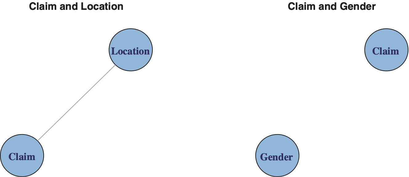
Exhibit 4.2 presents two graphs next to each other. The vertices (nodes) represent the variables. The presence of an edge (chord) between two nodes implies the variables are related. Absence of an edge implies independence.

To summarize, we can test for independence using either the Pearson chi-square test X², section 3, or use deviance G² as defined above for the log-linear model. Furthermore, we can represent our results by graphs as shown in Exhibit 4.2.

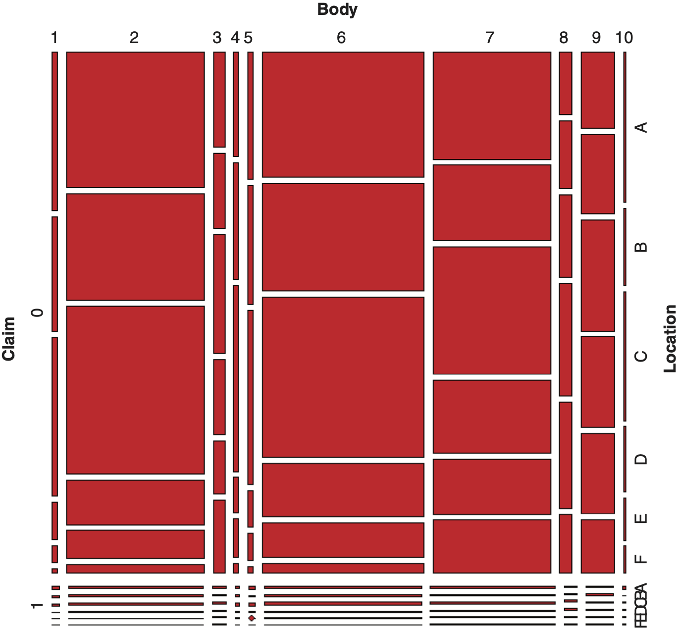
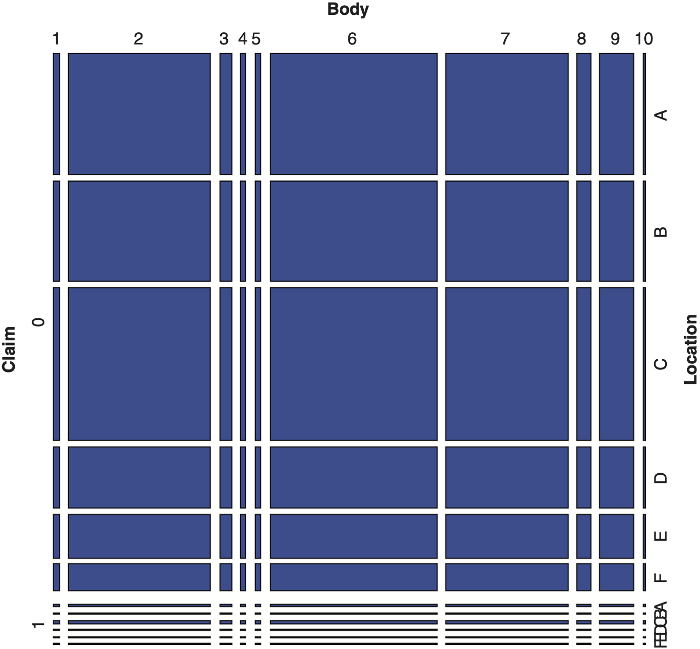
Next, we proceed to describe mosaic plots for visualizing a three-way contingency table. Table 4.1 summarizes the data for categorical variables Claim, Body and Location in the form of three-way contingency table derived from the Australian automobile insurance data.

Exhibit 4.3 displays a mosaic plot corresponding to Table 4.1.

Exhibit 4.3.Mosaic plot for Claim, Body and Location

The construction of the mosaic plot for the multidimensional contingency table, three categorical variables in this instance, is based on the exposition given by Friendly (1994).

For three categorical variables A, B, and C, with typical levels of j, k, and l, respectively, to each cell (j, k, l) of the three-way contingency table, there corresponds a tile (j, k, l) constructed by the following three sequential steps:

1. Step (1). For A, the first categorical variable, create vertical strips with width proportional to n_j++.

2. Step (2). Each vertical strip in Step (1) is sub-divided horizontally with height proportional to $\frac{n_{j k+}}{n_{j++}},$, conditional count of the second variable B given the first variable A.

3. Step (3). Each JK rectangle in Step (2) is further subdivided vertically with widths proportional to $\frac{n_{j k l}}{n_{j k+}}$

In this fashion, a tile constructed in Step (3), labeled as (j, k, l), has an area proportional to n_jkl.

These three steps above are analogous to writing the joint probability of the cell (j, k, l) as a product of marginal and conditional probabilities, as expressed by

$$\begin{array}{c} P(A=j, B=k, C=l) \\ =P(A=j) P(B=k \mid A=j) P(C=l \mid A=j, B=k) . \end{array}$$

Exhibit 4.4 shows the mosaic plot for the three categorical variables Claim, Body and Location based on the expected frequency under the assumption of independence. That is, the joint probability of the cell (j, k, l), p_jkl is computed as the product of three marginal probabilities, i.e., p_jkl = p_j++ p_+k+ p_++l. All probability items are estimated by appropriate cell count ratios.

Exhibit 4.4.Mosaic plot for Claim, Body and Location based on the hypothesis of independence

Applying log-linear models, the independence assumption was not supported for any of three categorical variables studied. Hence, it should not be surprising to see Exhibits 4.3 and 4.4 having different appearances.

As the number of categorical variables increases, then it becomes harder to interpret the pattern of dependency among variables based on mosaic displays. This is because the addition of a new variable requires further subdivision of each existing tile.

Now, we consider log-linear models for the case of three categorical variables A, B, and C. The notations previously used will be extended to the case of three.

A log-linear model for three categorical variables A, B, and C, with C having a typical value of l, where l ∈ dom(C) = {1, 2, . . . , L}, is defined by equation (3). The model in (3) is referred to as the saturated log-linear models for three categorical variables:

$$\begin{aligned} \log \left(m_{j k l}\right)= & u+u_{j}^{A}+u_{k}^{B}+u_{l}^{C}+u_{j k}^{A B} \\ & +u_{j l}^{A C}+u_{k l}^{B C}+u_{j k l}^{A B C}, \end{aligned} \tag{3}$$

where m_jkl is the expected count for the cell (j, k, l), with (j, k, l) ∈ dom(A) × dom(B) × dim(C); u is the constant (intercept) term, u_j^A, u_k^B, and u_l^C are the main effect terms, and u_jk^AB, u_jl^AC, u_kl^BC, and u_jkl^ABC are two-factor and three-factor interaction terms.

For a sample of size n, the random vector (A,B,C) has a multinomial distribution. The number of parameters in model (3) is overspecified and subject to constraint, as in the case of two categorical variables above.

The saturated model (3) is the largest model with respect to three categorical variables. By excluding certain u-terms in (3) above, alternative dependency structures among A, B, and C may be considered. The saturated model serves as a base model for comparing to other parsimonious log-linear models.

There are two subclasses of log-linear models which are of interest to us: the hierarchical models and the graphical models. The definition of these terms is based on the one given by Edwards (2000). In a hierarchical log-linear model, if a u-term is excluded (set equal to zero) then all its higher-order related u-terms are also excluded. Graphical models, a subclass of hierarchical models, are formed by excluding a set of two-factor interaction terms (and hence their higher-order related terms). For a more detailed discussion of these concepts, refer to Lauritizen (1996).

The independent model, the smallest log-linear model with all the three categorical variables included, is presented as:

$$\log \left(m_{j k l}\right)=u+u_{j}^{A}+u_{k}^{B}+u_{l}^{C} . \tag{4}$$

Among log-linear models, the conditionally independent models are of much interest. These models are not as detailed as the saturated model but provide additional dependency structure not provided by the independence model. They are easier to interpret and belong to the class of graphical models.

The conditional independence property, as it relates to three categorical variables A, B, and C, is defined as follows:

A and B are conditionally independent given C if

$$\begin{array}{c} P(A=j, B=k \mid C=l)= \\ P(A=j \mid C=l) P(B=k \mid C=l), \end{array}$$

for all (j, k, l) ∈ dom(A) × dom(B) × dim(C).

The notation used to express conditional independence, is A||B|C due to Dawid (1979).

The three conditional independence models of interest are:

$$\log \left(m_{j k l}\right)=u+u_{j}^{A}+u_{k}^{B}+u_{l}^{C}+u_{j l}^{A C}+u_{k l}^{B C} \tag{5a}$$

$$\log \left(m_{j k l}\right)=u+u_{j}^{A}+u_{k}^{B}+u_{l}^{C}+u_{j k}^{A B}+u_{k l}^{B C} \tag{5b}$$

$$\log \left(m_{j k l}\right)=u+u_{j}^{A}+u_{k}^{B}+u_{l}^{C}+u_{j k}^{A B}+u_{j l}^{A C} \tag{5c}$$

Using the conditional independence notation, we have A||B|C, A||C|B, and B||C|A corresponding to (5a), (5b), and (5c), respectively.

To discuss further the graphical models, we need to introduce some basic elements of graph theory. Graph theory is a branch of mathematics (see Berge [1962] 2001). Graph theory has been applied to transportation networks and social networks (Kolaczyk 2009) and used in computer science (see Cook and Holder 2007). For interaction of graph theory and log-linear models, refer to Whittaker (1990), Lauritzen (1996), and Edwards (2000).

A graph, G is a pair (V, E) where V is a finite set of vertices and E, a subset of V × V, is a set of edges. Here, the vertices represent variables, and for two vertices a and b such that (a, b) ∈ E implies a relationship between vertices a and b. If (a, b) ∈ E then we say that vertices a and b are adjacent to each other. A graph is simple if we exclude loops and multiple edges. A graph is undirected if (a, b) ∈ E implies (b, a) ∈ E. The graphs considered here are simple and undirected. A graph is complete if all the vertices in the graph are adjacent to each other.

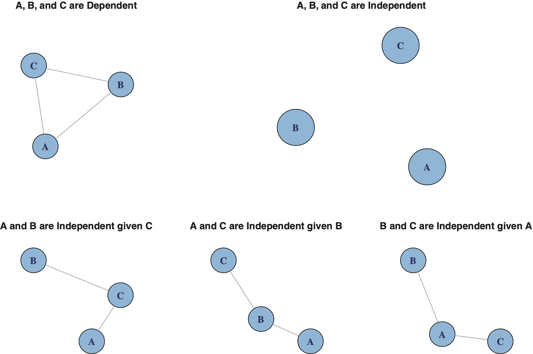
Exhibit 4.5 presents five graphs of interest corresponding to the models (3), (4) and (5) above.

Exhibit 4.5.Graphical models corresponding to complete, independent, and conditional independence

The top-left graph of Exhibit 4.5 corresponds to a graph that is complete, the saturated model of (3). The top-right graph with no edges corresponds to the independent model of (4). The three graphs in the lower part of the exhibit, from left to right, correspond to conditional independence models of A||B|C, A||C|B, and B||C|A, respectively, i.e., to (5a), (5b), and (5c).

Relative to the saturated model, a conditional independent model is a more parsimonious model in the sense that it requires fewer parameters to be specified. Furthermore, the conditional independent models are easier to explain and interpret graphically. For instance, the conditional independent model of (5b), A||C|B, implies that the edge AC has been removed from the complete model.

Returning to the Australian Auto data, with seven categorical variables, there are potentially 35 possible log-linear models involving three categorical variables.

Each of these 35 models failed the test of independence. Next, we considered the conditionally independent models, models (5a), (5b) and (5c), for the 35 cases. Exhibit 4.6 provides the summary of testing for the conditional independence where the results were statistically significant.

The function ciTest_table of the R package gRim (see Højsgaard, Edwards, and Lauritzen 2012) was used to perform the conditional independent tests. With three categorical variables, the implication of conditional independence test is tantamount to removal of an edge from the respective complete graph. Exhibit 4.7 provides the R output in the case of selected three variables: Claim, Gender, and Vehicle Age.

# Output of conditional independence test for
# Claim and Vehicle Age given Gender:

ciTest_table(d.3.245.table, set=c(“Claim”, “VehAge”, “Gender”))
Testing Claim _|_ VehAge | Gender
Statistic (DEV): 27.246 df: 6 p-value: 0.0001 method: CHISQ
# d.3.245.table: Data set for Claim, Vehicle Age and Gender

# Output of conditional independence test for
# Claim and Gender given Vehicle Age

ciTest_table(d.3.245.table, set=c(“Claim”, “Gender”, “VehAge”))
Testing Claim _|_ Gender | VehAge
Statistic (DEV): 1.225 df: 4 p-value: 0.8740 method: CHISQ
# d.3.245.table: Data set for Claim, Gender and Vehicle Age

# Output of conditional independence test for
# Vehicle Age and Gender given Claim

ciTest_table(d.3.245.table, set=c(“VehAge”, “Gender”, “Claim”))
Testing VehAge _|_ Gender | Claim
Statistic (DEV): 288.004 df: 6 p-value: 0.0000 method: CHISQ
# d.3.245.table: Data set for Claim, Gender and Vehicle Age

In Exhibit 4.7, the p-value for testing the conditional independence of Claim and Gender given the Vehicle Age is 0.8740. It has the implication that the test fails to reject the conditional independence test in this instance. Results in Exhibit 4.6 were similarly derived.

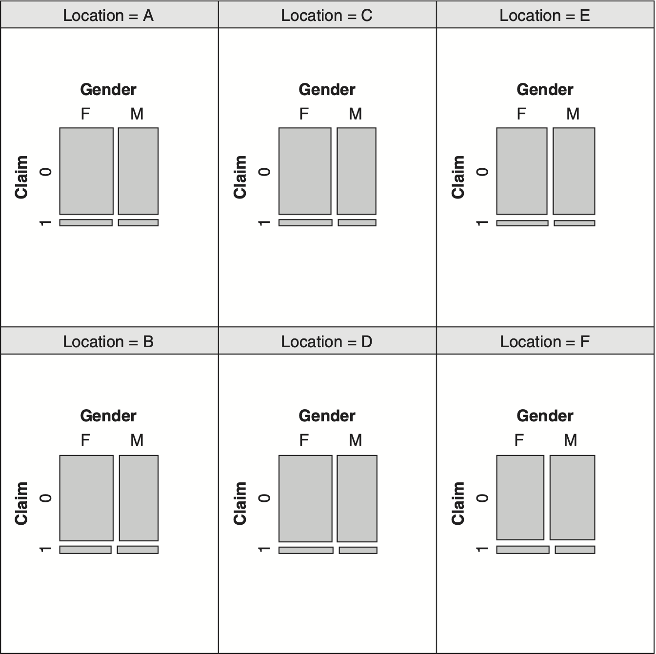
Before proceeding to the next section involving more than three categorical variables, it is worth introducing an additional exploratory tool for visualizing “conditional” relationship among three variables. Exhibit 4.8 displays the relationship between Claim and Gender for each level of Location variable.

Exhibit 4.8.Conditional plot of Claim and Gender given Location

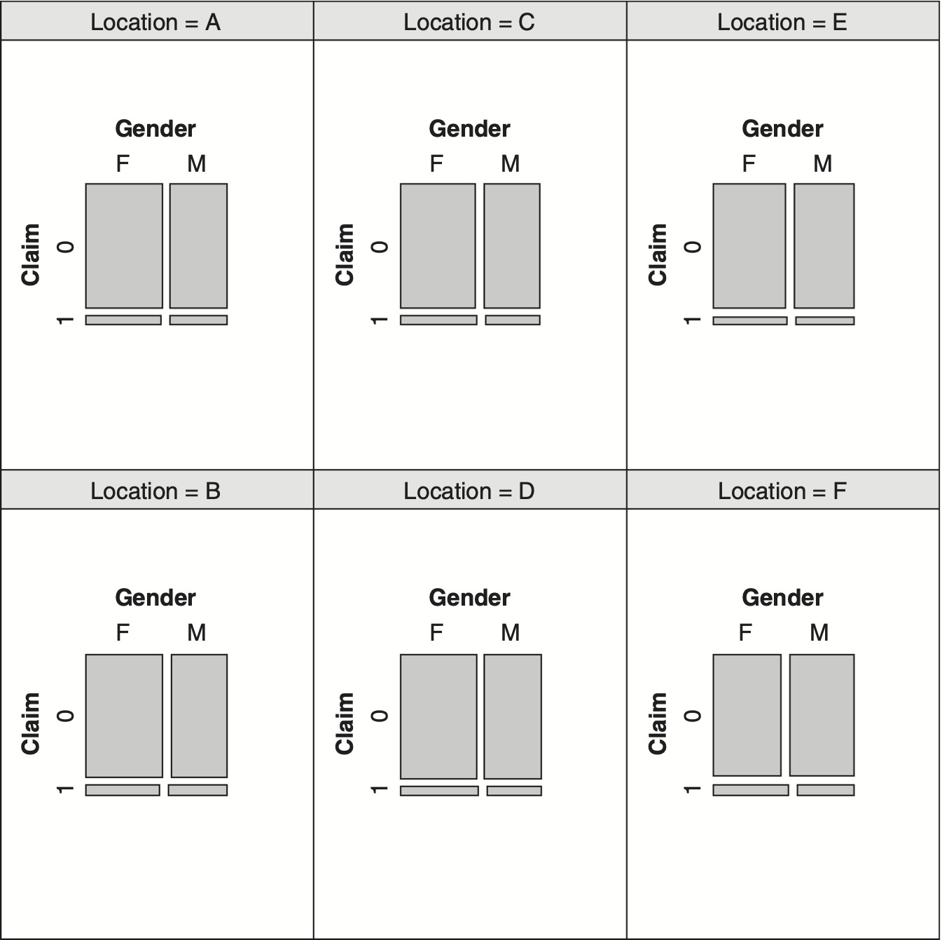
Reviewing the six panels of Exhibit 4.8, one notices the similarity of these panels with respect to Claim and Gender for each level of Location. This observation is consistent with formal test of conditional independence, case 5, of Exhibit 4.6.

5. Graphical models

Log-linear models of the previous section can be extended to more than three categorical variables. By increasing the number of variables, one encounters two kinds of problems. The first problem is referred to as the “model selection” and the second as the “estimation” problem. Let us elaborate on each of these two issues. By excluding certain two-factor, three-factor, or other higher order factor interaction terms, different log-linear models are obtained. The number of potential log-linear models increases in a non-linear fashion as the number of categorical variables increases. According to Christensen (1997), with four categorical variables there are 113 ANOVA type models with their main effects included. Furthermore, with five categorical variables, there are several thousand models to choose from. The model search space, the set of potentially acceptable log-linear models, is very large, and finding an “optimum” model among the potential models is a challenging task. It may be more expedient to search among the smaller class of graphical models for a suitable candidate. Graphical models have the advantage of being presented as graphs and are subject to easier interpretation.

The second problem is related to estimation of parameters of log-linear models. Some data sets have cells with zero frequency. In these situations, some software may either fail to fit a model to the data, or it may make adjustments and proceed to fit a model accordingly. The handling of empty cells is not uniform among different software. Hence, there are uncertainties regarding the output depending upon the software selected; see Højsgaard, Edwards, and Lauritzen (2012). Obtaining empty cells is not that uncommon when the number of categorical variables increases. With a fixed sample size, the observations need to be spread to a larger number of cells resulting in some cells being empty.

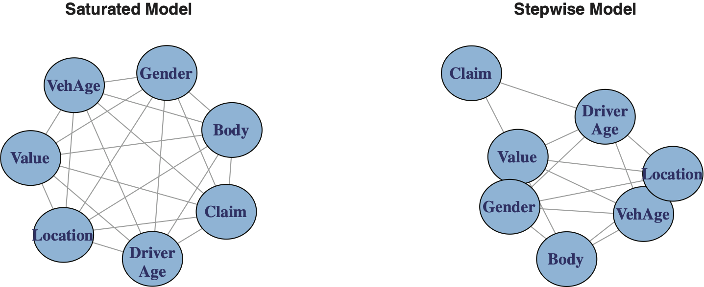
The approach in this paper for selecting a model is as follows. First, we fit a saturated model to the data using all the available categorical variables. The fitted saturated model corresponds to a complete graph. Here, we use the term model and graph interchangeably. The second step involves using the fitted saturated model as an input to the stepwise function of R in the gRim package. The output of the stepwise function is a more parsimonious fitted log-linear model belonging to the class of graphical models. The stepwise function uses a backward elimination procedure by removing certain edges of the saturated graph, thus producing a pruned subgraph; see Højsgaard, Edwards, and Lauritzen (2012).

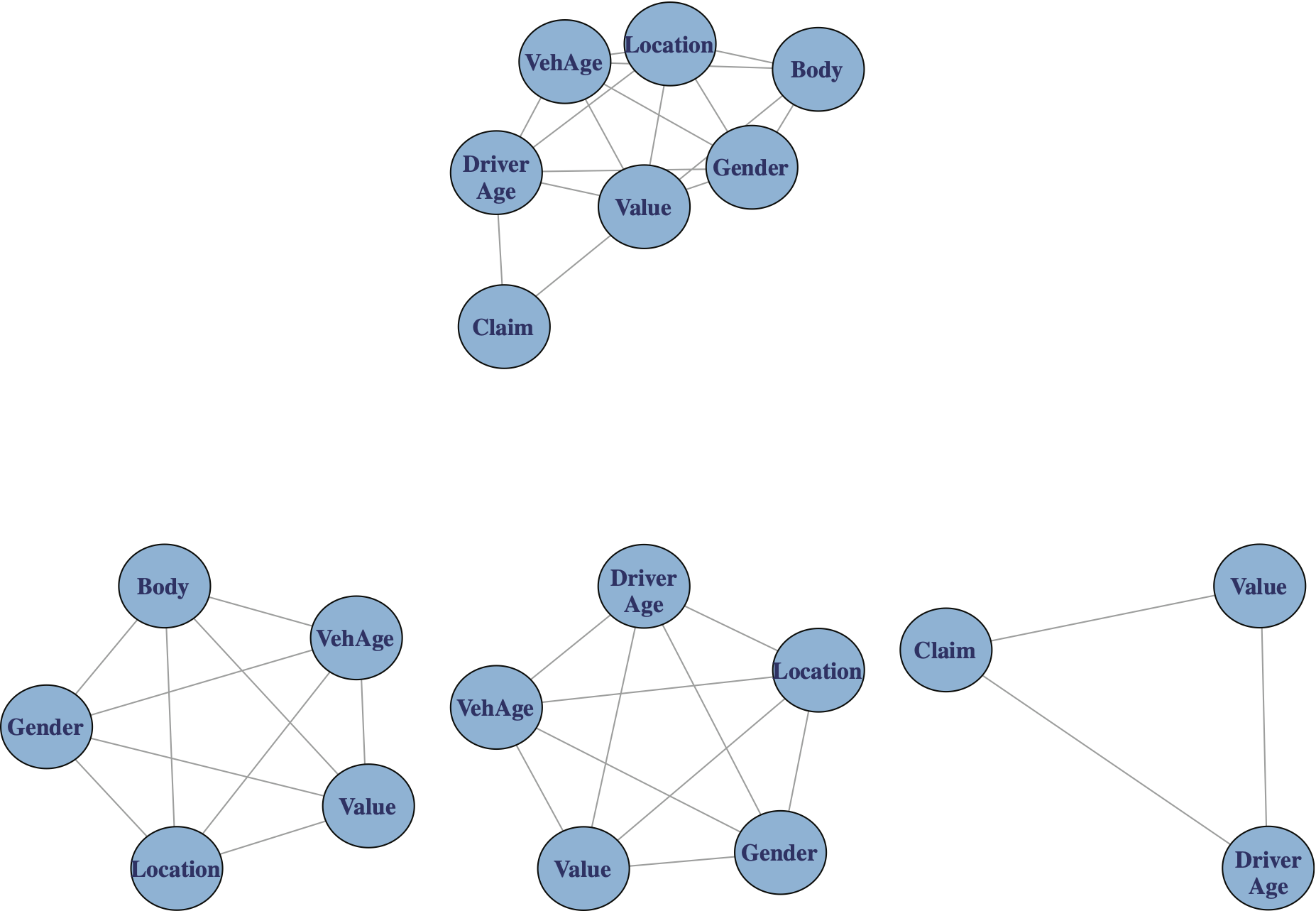
The graphs of the saturated fitted model and the graph produced by applying the stepwise function, here referred to as the stepwise model, are shown in Exhibit 5.1.

Exhibit 5.1.Graphical models for saturated and stepwise models based on the Australian Auto data

An insight into structure of the stepwise graph is provided by examining its cliques. A clique is a complete (maximal) subgraph such that by enlarging its vertex set, it would lose the property of being complete.

An intuitive characteristic of a clique based on the exposition of Hanneman and Riddle (2005) is as follows: a clique is a subgraph of a graph whose nodes are more closely and intensely related to one another than they are to other nodes of the graph.

Exhibit 5.2 illustrates the composition of three cliques associated with the graph of the fitted stepwise model.

Exhibit 5.3 illustrates the fitted stepwise model and its cliques.

Exhibit 5.3.Stepwise graph and its cliques

Two of the cliques of Exhibit 5.3 provide exposure (underwriting) information and the third clique, the lower right, provides claim information. Two of the cliques show a strong binding among the four variables Value, Vehicle Age, Gender and Location. By confining ourselves to graphical models, and examining their cliques, we can gain an insight into variables that are closely related.

We now give an example for reviewing claim frequency rates which utilizes the cliques given in Exhibit 5.2. Let us compute average Claim occurrence rate for each cell in three circumstances. The three cases depend upon which underwriting factors have been selected. We shall refer to these cases as “All,” “Clique 1,” and “Clique 2.” Table 5.1 gives a summary of the statistics produced. We shall explain the statistics corresponding to the “All” case. The figures for the other two cases were similarly computed.

For the Australian auto insurance, the “All” case involved the six underwriting variables. The variables involved were Value (after conversion from numeric to ordinal), Body (after reducing the number of level from 13 to 10), Vehicle Age, Gender, Location, and Driver Age. The number of potentially distinct cells arising from different combination of levels of these six variables was 11,520 (4 * 10 * 4 * 2 * 6 * 6). The actual number of non-empty observed cells was 5,063. The average value of Claim occurrence for each cell, referred to as rate, was computed. Only 1,905 cells had positive average Claim occurrence rates. These positive claim rates may be utilized for computing or reviewing frequency rates. Note that the traditional ratemaking procedures may not consider some of these 1,905 cell rates as credible due to low cell counts. Regarding these positive average Claim occurrence rates, we computed the values of Minimum, Q1 (first quantile), Median, Mean, Q3 (third quartile) and Maximum (see Table 5.1). The figures for “Clique 1” and “Clique 2” cases were similarly determined.

For the above three cases, we constructed boxplots to compare the distribution of positive average Claim occurrence rates; see Exhibit 5.4.

Exhibit 5.4.Comparison of average claims rates

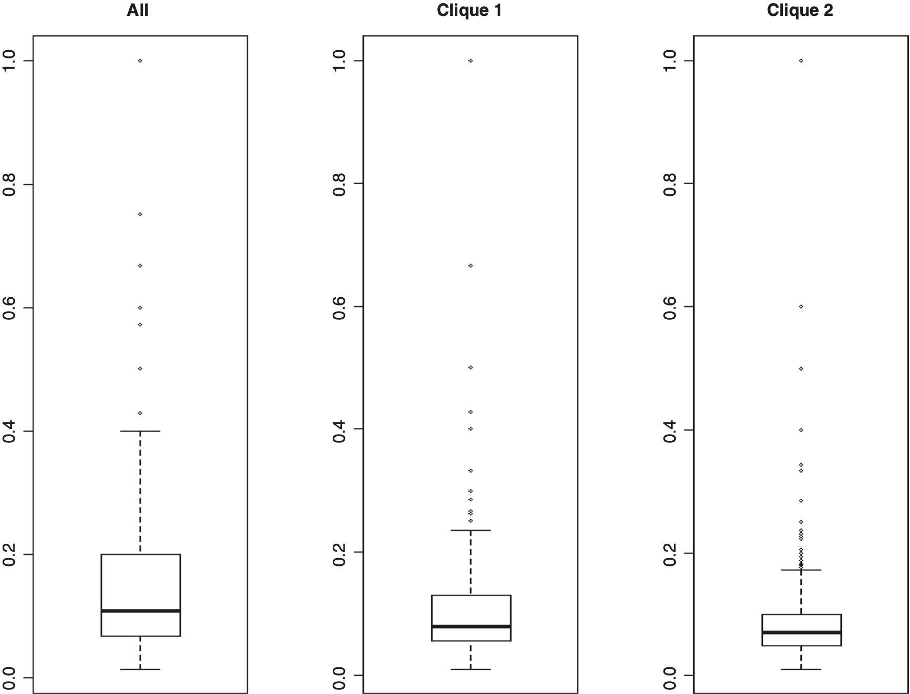
Reviewing the boxplots, we note that “frequency” rates for the “Clique 2” are more stable. They are less volatile, and the median and mean values are close to each other. For “All” and “Clique 1” cases, the average Claim occurrence rates may well be influenced by outliers. It is difficult to visually see the number of outliers appearing in Exhibit 5.4. I used the “out” attribute of the R boxplot function for determining outliers (extremes); see the following link: http://stat.ethz.ch/R-manual/R-devel/library/grDevices/html/boxplot.stats.html.

The outlier definition used is associated with the “out” attribute of the boxplot function defined as “the values of any data points which lie beyond the extremes of the whiskers.” The percentage of outlier values for the “All,” “Clique 1,” and “Clique 2” were 10.4, 11.1, and 5.2, respectively. Our example may help in determining or reviewing a collection of “frequency” rates which are more stable and are based on smaller number of rating factors.

Finally, we shall discuss briefly the notion of overfitting as it applies here. The graphs in Exhibit 5.3 were based on using the entire data set. Results based on using all data may be too “optimistic”—close to the data—and may not necessarily generalize well to similar unseen data. This phenomenon is referred to as overfitting. Tan, Steinbach, and Kumar (2006) discuss overfitting as it applies to classification, a supervised learning task. As was mentioned above, our study is mainly an exercise in unsupervised learning, and, moreover, we did not have access to similar additional unseen data. So, to validate our findings regarding the stepwise graph and its cliques (Exhibit 5.3), we considered replicating our results by selecting 10 random samples of equal size from the original data set. For each random sample (1) we determined the fitted saturated model, (2) used the sample fitted saturated model as input to the stepwise function to determine the corresponding fitted stepwise model, and (3) examined the cliques associated with fitted stepwise model for each of the 10 samples. The result of these replications is summarized in Table 5.2.

Reviewing the results in Table 5.2, we note that using the entire data set produced two cliques of size 5 which do not appear among the cliques produced by the 10 replications. This result may be attributable to the size effect. It is conceivable that a pattern observed in a large data set may not reveal itself in smaller data sets (see Mayer-Schonberger and Cukier 2013). But the two cliques of size 4 from the replicated samples share the same variables as the cliques of size 5 based on the entire data. It is interesting to note that the cliques involving the three variables Location, Value and Vehicle Age appeared in all 10 random samples. Overall, the results obtained by performing the replications do not appear to contradict the findings based on the entire data.

6. Summary and concluding remarks

In this paper, we studied several categorical variables related to an Australian automobile insurance data. We began by using exploratory data analysis tools to understand the nature of our data. We transformed of some of the variables as a part of preprocessing the data. Visualization tools—bar charts, mosaics, and conditional plots—were informally used. We constructed several multi-dimensional contingency tables for summarizing the information regarding the categorical variables used.

Tests of independence based on chi-square statistic and log-linear models were discussed. Concepts of conditional independence and graphical modeling were introduced. By examining the cliques of a parsimonious graphical model fitted to the data, one obtains insight into which combination of categorical variables tend to bind together. Furthermore, we discussed briefly issues related to model selection and overfitting. Finally, an example was given that utilized the information provided by cliques of a fitted graphical model regarding dependency structure among rating variables. Such an analysis may supplement the traditional ratemaking reviews of classification rates.