A Comparison of Two Individual Tree-Based Loss Reserving Methods

undefined

1. Introduction

Non-life insurers face high volatility due to the nature of the losses they must provide coverage for. Regulation thus requires them to maintain funds under solvency constraints to ensure that there will be a minimal probability of being insolvent up to a particular risk level. Precise guidelines exist to determine the capital required for an insurer varying from one country or state/province to another. For property and casualty insurance companies, United States regulation as defined by the National Association of Insurance Commissioners uses risk-based capital requirements (see Feldblum 1996), while the Canadian requirement is set forth as the conditional tail expectation (CTE) at a $99~\%$ level for insurance risk (Office of the Superintendent of Financial Institutions 2018).

There are many classical (or aggregate) methods to evaluate such reserves; see Wüthrich and Merz (2008) and Friedland (2010) for an extensive discussion of existing methods. However, individual loss reserving approaches, traced to the 1980s with the development of a mathematical framework in continuous time by Arjas (1989) and Norberg (1986), have received much attention in recent years. Many approaches have been proposed, e.g., Larsen (2007), Zhao, Zhou, and Wang (2009), Pigeon, Antonio, and Denuit (2013), and Antonio and Plat (2014). On the one hand, statistical learning techniques are widely used in data analytics. On the other hand, only a few approaches based on these techniques, mainly tree-based machine learning methods and neural networks, have been developed in loss reserving using micro-level information. A reader interested in a broader view of the subject can consult Taylor (2019). It presents the evolution of loss reserving methods focusing on recent individual loss reserving methodologies and machine learning approaches. Comparisons are made, highlighting their strong points and guiding the choice of an optimal strategy. In particular, several approaches based on decision trees have been proposed recently, with real practical potential. Consequently, we concentrate on tree-based machine learning methods.

As far as we know, Wüthrich (2018) is the first paper to apply a tree-based machine learning method, the well-known Classification And Regression Tree (CART) algorithm introduced by Breiman et al. (1984), in an individual loss reserving framework. This paper considers regression trees in a discrete context to only predict the number of payments. First, the numbers of payments for reported but not settled (RBNS) claims are predicted using feature components on an individual basis. Second, incurred but not reported (IBNR) claims are considered. For such claims, individual claim-specific information is unknown; hence no individual predictions can be obtained. Wüthrich (2018) assumes that claim occurrences and the reporting process can be described by a homogeneous marked Poisson point process enabling him to apply the Chain-Ladder method to obtain the predictions. Then, predictions for closed claims, RBNS claims, and IBNR claims are aggregated to obtain a prediction of all payments for all accident years. Finally, a prediction for the final reserve amount can be calculated based on these predictions.

The work of Wüthrich (2018) is the foundation of the work of De Felice and Moriconi (2019), which also uses CART within their prediction model. Contrary to Wüthrich (2018), paid amounts are considered within a frequency-severity model. CARTs are applied in both the frequency (classification trees) and severity (regression trees) predictions. An essential addition in this work is an assumption of multiple payment types, meaning that different regimes are used to handle incurred claims. This double-claim regime allowing two different types of compensation for the same claim is shown to be suitable in an application to Italian Motor Third Party Liability data given that incurred claims here can be handled under two regimes: direct compensation and indirect compensation.

Baudry and Robert (2019) proposed a general recursive approach based on Extremely randomized trees (ExtraTrees) to assess outstanding liabilities based on all available information since the reporting of the claim. Applications are made for specific recursive one-period ahead predictions as in the framework proposed by Wüthrich (2018).

Many of those individual loss reserving methodologies presuppose the availability of many closed files, i.e., files for which the full development of the claim—from the occurrence until the final closure of the file—is known. In practice, this assumption is never verified, and the actuary must include open files in the modeling process. This remark is not unique to the valuation of reserves or actuarial science but is found in many fields, such as biostatistics or epidemiology. There are generally two families of approaches to resolving this problem: (A) strategies based on survival analysis and (B) strategies based on the imputation of missing data. Recently, two propositions have been developed in the actuarial literature, each belonging to one of these families. They make it possible to include open files in the individual modeling of loss reserves.

As part of the (A) family, Lopez, Milhaud, and Thérond (2016, 2019) propose an adaptation of the CART algorithm to censored data (open claims) and implement the procedure to obtain ultimate individual reserves for RBNS claims. This extension of the CART algorithm introduces a weighting scheme based on a Kaplan-Meier estimator to compensate for the censoring of the data in the sample. More precisely, a weighted quadratic loss is used as a splitting criterion rather than the quadratic loss of the classical CART algorithm (we describe this approach in Section 3). In Lopez (2019), a construction based on copulas is introduced in a model similar to the one proposed in Lopez, Milhaud, and Thérond (2016) based on survival analysis to account for a possible dependence between the length of time from the occurrence to the closure of a claim and the amount of the claim.

Belonging to the (B) family, Duval and Pigeon (2019) propose an individual loss reserving model based on an application of the gradient boosting algorithm, more precisely, the XGBoost algorithm. Based on the prediction distribution of the RBNS claims, they compare this non-parametric approach using a machine learning algorithm with more classical reserving techniques such as a bootstrapped version of Mack’s collective model (see England and Verrall 2002), a collective generalized linear model (GLM) (see Wüthrich and Merz 2008) and an individual GLM loss reserving model.

The main objective of this paper is to investigate the strategies proposed in Lopez, Milhaud, and Thérond (2016, 2019) and Duval and Pigeon (2019) to include open files within the loss reserving process. These two propositions were developed in parallel and have never been compared. We analyze challenges faced by integrating open claims into an individual reserve valuation process, and we compare their performance to classical aggregate loss reserving methods based on sampled datasets. To the best of our knowledge, this is one of the first times that a comparative study of several individual approaches is performed from simulated data. Therefore, it is fully transparent and reproducible.

The paper is structured as follows. In Section 2, we define both individual and collective frameworks for loss reserving and define the loss reserving problem under study. In Section 3, we present in detail approaches proposed in Lopez, Milhaud, and Thérond (2016) and Duval and Pigeon (2019) to include open files in the modeling process. We perform many simulation studies in Section 4, and finally, we conclude and present some remarks in Section 5.

2. Individual Loss Reserving

In property and casualty insurance, a claim starts with an accident happening at the occurrence point (see Figure 2). For some situations, e.g., for bodily injury liability coverage, a reporting delay is observed between the occurrence date and the reporting to the insurance company at the reporting point. At this moment, the insurer could observe details about the accident and some information about the insured. A series of random payments are triggered from this moment until the closing date of the file. We illustrate in Figure 1 the development of four individual claims.

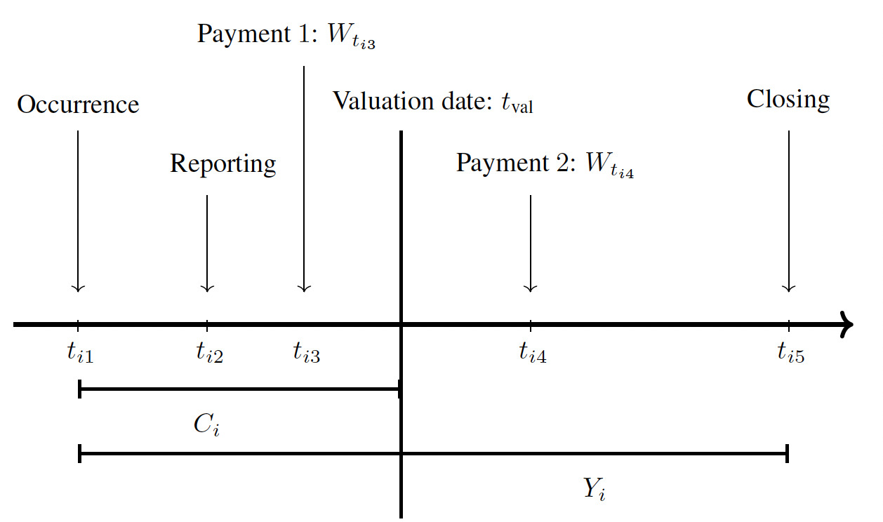
The valuation date $t_\text{val}$ is the moment at which the insurance company wants to evaluate its solvency and calculate reserves. At this date, we may classify each claim according to the usual categories in the loss reserving literature: Incurred But Not Reported, or IBNR; Reported But Not Settled, or RBNS; and Closed. The paper mainly focuses on RBNS claims, i.e., claims for which the accident has been reported to the insurer, but the file still needs to be settled.

We have kept the notation as close as possible to the one used in survival analysis and censored data analysis to facilitate parallels between the various sources. Let

• $\{Y_1, \ldots, Y_n\}$ be a random sample^[1] of duration random variables from an unknown cumulative distribution function (cdf) $F: \mathbb{R}^+ \to [0,1]$. In the context of loss reserving, $Y_i$ is the time elapsed between the occurrence and closure dates for claim $i$.

• $\{M_1, \ldots, M_n\}$ be a set of random variables $M_i \in \mathbb{R}$, $i = 1, \ldots, n$ representing the total paid amount for the $i^{\text{th}}$ claim.

• $\{C_1, \ldots, C_n\}$ be a random sample from an unknown censoring cdf $G$. The censoring variable $C_i$ is the delay between the occurrence and valuation dates. Consequently, open and closed claims are considered censored and uncensored observations, respectively.

• $\{\pmb{x}_1, \ldots, \pmb{x}_n\}$ be a set of covariates, $\pmb{x}_i \in \mathcal{X} \subset \mathbb{R}^p$, $i = 1, \ldots, n$.

We define

$$\begin{aligned} Z_i &= \min(Y_i, C_i), \quad \delta_i = \mathbb{I}\left(Y_i \leq C_i\right), \end{aligned}$$

where $\mathbb{I}\left(Y_i \leq C_i\right) = 1$ if $Y_i \leq C_i$ and $0$ elsewhere, and $N_i = \delta_iM_i$. Thus, $Z_i$ and $N_i$ represent, for claim $i$, the duration and severity observed in the database at the valuation date. Without loss of generality, we assume that $Z_1 < Z_2 < \cdots < Z_n$, with $\delta_i$ and $N_i$, $i = 1, \ldots, n$, constructed accordingly. In this general framework, $(M_i, Y_i)$ may not be observed due to the censoring effect of $C_i$, but $\pmb{x}_i$ are always observed. Thus, in a dataset, we have $\{N_i, Z_i, \delta_i, \pmb{x}_i\}_{i=1, \ldots, n}$. Finally, we assume that $C_i$ is independent of $(Y_i, M_i)$, and

$$\operatorname{Pr}\left(Y_i \leq C_i \mid M_i, Y_i, \pmb{x}_i\right)=\operatorname{Pr}\left(Y_i \leq C_i \mid Y_i, \pmb{x}_i\right),$$

for $1 \leq i \leq n$.

Based on that, the main objective is to construct an estimator for

$$\begin{aligned} \pi_0 &= \text{argmin}_{\pi \in \mathcal{P}} \mathbb{E}[{\phi\left(M, \pi(Y, \pmb{x})\right]}, \end{aligned} \tag{1}$$

where $\mathcal{P}$ is an appropriate subset of a functional space and $\phi$ is a loss function. Informally, this means that we are looking for the function $\pi$ which minimizes a loss function $\phi$ calculated between $M$ on one side (the total paid amount for one claim in the loss reserving context) and $(Y, \pmb{x})$ on the other side (the settlement delay and all covariates in our case). Using the quadratic loss function and $\mathcal{P} = L^2(\mathbb{R}^p)$ or $L^2(\mathbb{R}^{p+1})$, we obtain the classical mean regression model where

$$\pi_0=\mathbb{E}[M \mid \pmb{x}] \text { or } \pi_0=\mathbb{E}[M \mid Y, \pmb{x}].$$

In the actuarial literature, censored variables are often discussed when a contract has a limit or deductible. It is important to note that in this paper, we are only interested in the censorship present in the duration of a file, and censored data corresponds to an open claim at the valuation date.

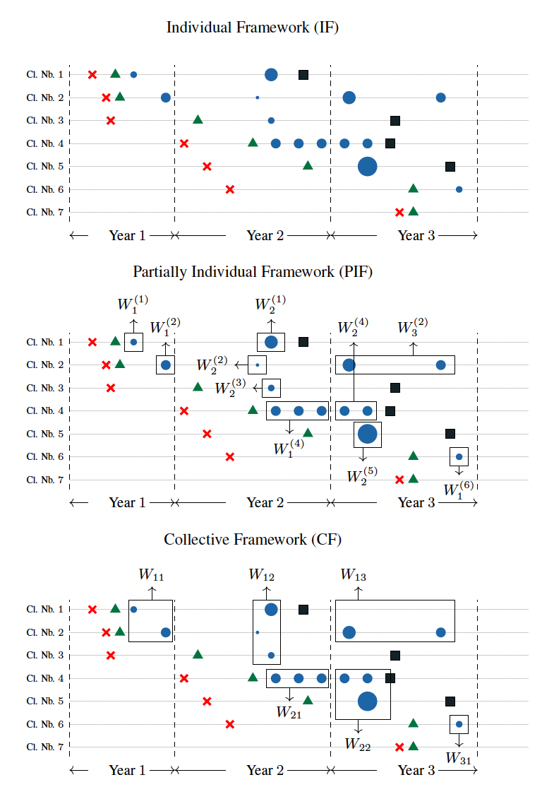
Based on this notation, it is now possible to define the valuation of the reserve according to the granularity, or level of aggregation, of the underlying database. In what follows, we distinguish three frameworks: individual, collective, and partially individual. We illustrate these $3$ frameworks in Figure 3.

Individual framework. Figure 2 illustrates the structure of the development of an individual claim with

$$M_i=W_{t_{i3}}+W_{t_{i4}} \text { and } N_i=0.$$

In the loss reserving framework, our main objective is to construct an estimator $\widehat{M}_i$ for

$$\mathbb{E}\left[M_i \mid N_i, Z_i, \delta_i, \pmb{x}_i\right],$$

which is the best $L^2$-predictor of the total paid amount $M_i$. We call this approach the purely individual framework (IF). A prediction of the RBNS reserve amount is given by

$$\begin{aligned} \widehat{R}^{\text{RBNS}} &= \sum_{i=1}^n \left(\widehat{M}_i - m_i^*\right), \end{aligned}$$

where $m_i^*$ is the observed total paid amount at the valuation date for claim $i$. It should be noted that for closed files, we have $\widehat{M}_i = m_i^*$.

Collective framework. Traditionally, insurance companies aggregate information by accident year and by development year. Claims with accident year $a$, $a = 1, \ldots, J$, are all claims that occurred in the $a{\text{th}}$ year after $\tau$, an ad hoc starting point common to all claims. For a claim $i$, a payment made in development year $j$, $j = 1, \ldots, J$ is a payment made in the $j{\text{th}}$ year after the occurrence $t_{i1}$, namely a payment $W_{t_{im}}$ for which $j - 1 < t_{im} - t_{i1} < j$. For development years $j = 1, \ldots, J$, we define

$$\begin{aligned} W_j^{(i)} &= \sum_{m \in \mathcal{S}_j^{(i)}} W_{t_{im}}, \end{aligned}$$

where $\mathcal{S}_j^{(i)} = \{m:j - 1 < t_{im} - t_{i1} < j\}$, as the total paid amount for claim $i$ during year $j$ and we define the corresponding cumulative paid amount as

$$\begin{aligned} C_j^{(i)} = \sum_{s = 1}^j W_s^{(i)}. \end{aligned}$$

A collective approach groups every claim in the same accident year to form the aggregate incremental payment

$$\begin{aligned} W_{aj} &= \sum_{i \in \mathcal{K}_a} W_j^{(i)}, \qquad a,j = 1, \ldots, J, \end{aligned}$$

where $\mathcal{K}_a$ is the set of all claims with accident year $a$. For portfolio-level models, a prediction of the reserve is obtained by

$$\begin{aligned} \widehat{R}^{\text{RBNS} + \text{IBNR}} &= \sum_{a = 2}^J \sum_{j = J + 2 - a}^J \widehat{W}_{aj}, \end{aligned}\tag{2}$$

where the $\widehat{W}_{aj}$ are usually predicted using only the accident year and the development year. It is the collective framework (CF). It is worth noting that this framework does not allow distinguishing the RBNS reserve from the IBNR reserve.

Partially individual framework (PIF). In the collective framework, each cell contains a series of payments, information about the claims, and some information about policyholders. These payments can also be modeled within an individual framework. Hence, a prediction of the total reserve amount is given by

$$\begin{aligned} \widehat{R}^{\text{RBNS} + \text{IBNR}} &= \underbrace{\sum_{a = 2}^J \sum_{j = J + 2 - a}^J \sum_{i \in \mathcal{K}_a} \widehat{W}_{j}^{(i)}}_{\text{RBNS reserve}} \\ &\quad+ \underbrace{\sum_{a = 2}^J \sum_{j = J + 2 - a}^J \sum_{i \in \mathcal{K}_a^{\text{unobs.}}} \widehat{W}_{j}^{(i)}}_{\text{IBNR reserve}}, \end{aligned} \tag{3}$$

where $\mathcal{K}_a^{\text{unobs.}}$ is the set of IBNR claims with occurrence year $a$. It should be noted that in Equations (2) and (3), we assume that there will be no future payments on claims in the earliest occurrence period ($a = 1$). We call this approach the partially individual framework (PIF) because a partial aggregation of the information is made (by development period). However, for the remaining part, the information has been preserved. In this work, we are mainly interested in the reserve associated with the claims in the database: the RBNS reserve, which is the first part on the right-hand side of Equation (3).

3. Two Individual Tree-Based Models

Assume we have a portfolio $\mathcal{S}$ on which we want to train a model for loss reserving. This portfolio contains open and closed files that are important to consider in our modeling process. Considering only non-censored claims, or closed files, in the training set leads to building the model using a too high proportion of “simple cases” and underestimating the risk associated with the portfolio. This result was clearly shown in Duval and Pigeon (2019). In the context of this paper, we present two tree-based models recently developed in the actuarial literature. Each of these models is based on the CART algorithm (Breiman et al. 1984) and uses a different strategy to include open cases: correcting the selection bias using an inverse probability of censoring weighting strategy (see Subsection 3.1) and developing censored claims using a classical model before applying a statistical learning-based model (see Subsection 3.2). Finally, it is worth noting that we present a toy example of these two approaches in Appendix B to help clarify these two models.

Because both models are based on trees, we start by recalling how trees are generally constructed. Subsequently, we will present how the two models use this algorithm and how they include open files. To start, we assume that at each step $s \in \{1, 2, \ldots\}$ of the construction of a tree, the latter contains $L^{(s)}$ leaves $\{\mathcal{T}^{(s)}_j\}_{j = 1, \ldots, L^{(s)}}$ which are a partition^[2] of the space $\mathcal{T} = \mathbb{R}^+ \times \mathcal{X}$. An observation $\widetilde{\pmb{X}}_i = (Y_i, \pmb{X}_i)$ belongs to the leaf $\ell$ if $\widetilde{\pmb{X}}_i \in \mathcal{T}_\ell^{(s)}$.

• Step 1: Construction of the maximal tree. At the beginning of the algorithm ($s =1$), there is only one leaf in the tree corresponding to the set of all uncensored observations. A new tree ($s+1$) is created at each subsequent step by dividing one of the existing leaves. For the leaf $\ell$, this split is made based on an optimization: (1) for each covariate $x^{(j)}$ (the $j^{\text{th}}$ component of $\widetilde{\pmb{x}}$), one determines the threshold $x_\ell^{(j)}$ that minimizes the function $\mathcal{L}_\ell(j, x^{(j)}_\ell)$ defined by

  $$\small{\begin{aligned} & \mathcal{L}_{\ell}\left(j, x_{\ell}^{(j)}\right)= \\ & \quad \min _{\left(\pi, \pi^{\prime}\right) \in \Gamma^2} \int \phi(m, \pi) \mathbb{I}\left(\tilde{\pmb{x}} \in \mathcal{T}_{\ell}^{(s)}\right) \mathbb{I}\left(x^{(j)} \leq x_{\ell}^{(j)}\right) d \widehat{F}_n(m, \widetilde{\pmb{x}}) \\ & \quad+\int \phi\left(m, \pi^{\prime}\right) \mathbb{I}\left(\tilde{\pmb{x}} \in \mathcal{T}_{\ell}^{(s)}\right) \mathbb{I}\left(x^{(j)}>x_{\ell}^{(j)}\right) d \widehat{F}_n(m, \tilde{\pmb{x}}), \end{aligned} }$$

  where $\phi$ is a loss function, and $\Gamma \subset \mathbb{R}$; (2) determines

  $$j_0=\operatorname{argmin}_{j=1, \ldots, p+1}\left(\mathcal{L}_{\ell}\left(j, x_{\ell}^{(j)}\right)\right) .$$

  Finally, two new leaves are created by applying the splitting rule: $x_i^{(j_0)} \leq x_\ell^{(j_0)}$ and $x_i^{(j_0)} > x_\ell^{(j_0)}$. The empirical distribution function $\widehat{F}_n$ can be easily calculated without censored data. However, in the presence of censorship, this distribution is unavailable. The procedure ends when only one uncensored observation is left in each leaf or when all the uncensored observations in the same leaf are identical. This entire step can be performed using the rpart function available in the rpart package.

• Step 2: Pruning the tree. Let $K \leq n$ be the number of leaves in the maximal tree. The final tree is a sub-tree $S$, with $K_S \leq K$ leaves, selected from the set $\mathcal{S}$ of all sub-trees of the maximal tree. The pruning strategy is based on the following optimization problem:

  $$S(\alpha)=\operatorname{argmin}_{S \in \mathcal{S}}\left(\int \phi\left(m, \widehat{\pi}^S\right) d \widehat{F}_n(m, \tilde{\pmb{x}})+\frac{\alpha K_S}{n}\right),$$

  where

  $$\begin{aligned} \widehat{\pi}^S & =\sum_{\ell=1}^{K_S} \widehat{\gamma}_{\ell} R_{\ell}(\tilde{\pmb{x}}), \\ \widehat{\gamma}_{\ell} & =\operatorname{argmin}_{\pi \in \Gamma} \int \phi(m, \pi) R_{\ell}(\tilde{\pmb{x}}) d \widehat{F}_n(m, \tilde{\pmb{x}}), \end{aligned}$$ and $$R_{\ell}(\widetilde{\pmb{x}})=\mathbb{I}\left((\widetilde{\pmb{x}}) \in \mathcal{T}_{\ell}\right).$$

  In order to determine the optimal value of $\alpha$, $\alpha^*$, a cross-validation procedure is applied. Again, this procedure can be implemented directly using the xval argument of the rpart function.

Finally, the estimator of $\pi_0$ defined by Equation (1) is given by

$$\begin{aligned} \widehat{M} = \widehat{\pi}^{S(\alpha^*)} &= \sum_{\ell = 1}^{K_{S(\alpha^*)}} \widehat{\gamma}_\ell R_\ell(\widetilde{\pmb{x}}). \end{aligned}$$

As mentioned, in the context of loss reserving, the challenge comes from the unavailability of $\widehat{F}_n(m, \widetilde{\pmb{x}}) = \widehat{F}_n(m, y, \pmb{x})$ in the presence of censored data (open claims).

3.1. First Model Based on Survival Analysis

This section introduces the main ideas of the weighted regression tree procedure for censored data proposed in Lopez, Milhaud, and Thérond (2016). The authors explain in detail the theoretical bases of their approach and demonstrate the consistency of the estimator obtained. In the presence of censorship, they suggest replacing $\widehat{F}_n(m, y, \pmb{x})$ (in Step 1 and Step 2) by

$$\begin{align} \tilde{F}(m, y, \pmb{x})&=\frac{1}{n} \sum_{k=1}^n \frac{\delta_k \mathbb{I}\left(N_k \leq m, Z_k \leq y, \pmb{x}_k \leq \pmb{x}\right)}{\left(1-\widehat{G}\left(Z_k^{-}\right)\right)}\\ &=\sum_{k=1}^n w_k \mathbb{I}\left(N_k \leq m, Z_k \leq y, \pmb{x}_k \leq \pmb{x}\right), \end{align}$$

where $\widehat{G}$ is given by

$$\widehat{G}\left(Z_k^{-}\right)=1-\prod_{i=1}^{k-1}\left(\frac{n-i}{n-i+1}\right)^{1-\delta_i} \tag{4}$$

and

$$\begin{align} w_k&=\left(\frac{\delta_k}{n-k+1}\right) \prod_{i=1}^{k-1}\left(\frac{n-i}{n-i+1}\right)^{\delta_i}, \\ k&=2, \ldots, n-1, \end{align} \tag{5}$$

with $w_1 = \delta_1/n$, and $w_n= \prod_{i=1}^{n-1}\left(\frac{n-i}{n-i+1}\right)^{\delta_i}$. See Appendix A for the details on the Kaplan-Meier weights $w_j$.

Moreover, in order to determine the optimal value of $\alpha$ (Step 2), they propose a cross-validation procedure minimizing

$$\sum_{j=1}^{n^*} \frac{\delta_j \phi\left(N_j, \widehat{\pi}^{S(\alpha)}\right)}{1-\widehat{G}\left(Z_j^{-}\right)}.$$

For closed claims ($\delta_i = 1$), we simply have $\widehat{M}_i = m_i^*$, the observed total paid amount. For $\delta_i = 0$, several estimators are possible. Here we focus on two of the main ones. The first one is based on

$$\begin{aligned} M_i^{(1)}&=M_i^{(1)}\left(m_i^*, z_i, \pmb{x}_i\right)\\ &=\mathbb{E}\left[M_i \mid M_i>m_i^*, Y_i>z_i, \pmb{x}_i\right] \\& =\frac{\mathbb{E}\left[M_i \mathbb{I}\left(M_i>m_i^*, Y_i>z_i\right) \mid \pmb{x}_i\right]}{\operatorname{Pr}\left(M_i>m_i^*, Y_i>z_i \mid \pmb{x}_i\right)} \\ & =\frac{\mathbb{E}\left[\psi_2\left(m_i^*, z_i\right) \mid \pmb{x}_i\right]}{\mathbb{E}\left[\psi_1\left(m_i^*, z_i\right) \mid \pmb{x}_i\right]} \\ & =\frac{\pi_2\left(\pmb{x}_i\right)}{\pi_1\left(\pmb{x}_i\right)}, \end{aligned}$$

where $\psi_1(m, z) = \mathbb{I}(M > m, Y>z)$ and $\psi_2(m, z) = M\psi_1(m,z)$. In Lopez, Milhaud, and Thérond (2019), the authors propose to define

$$\begin{aligned} \widehat{M}_i^{(1)} &= \frac{\widehat{\pi}_{2}(\pmb{x}_i)}{\widehat{\pi}_{1}(\pmb{x}_i)}, \end{aligned} \tag{6}$$

where both estimators are constructed using the regression tree procedure introduced previously with Kaplan-Meier weights. These weights equal $0$ for open (censored) claims; otherwise, the larger the delay between the occurrence date and the valuation date, the higher the weight. It compensates for the fact that only a few claims with large observed development are observed in a dataset.

A second strategy is using one single tree and directly estimating

$$\begin{align} M_i^{(2)}&=M_i^{(2)}\left(N_i, Y_i, \pmb{x}_i\right)\\ &=\pi_5\left(\pmb{x}_i, N_i, Y_i\right)\\ &=\mathbb{E}\left[M_i \mid N_i, Y_i, \pmb{x}_i\right] . \end{align}$$

Because $Y_i$ is unknown for open claims (censored), we need, as a preliminary step, to obtain a predicted value $\widehat{y}_i$. Thus, the steps are

1. construct a model for $\left(Y_i|Y_i \geq z_i, \pmb{x}_i\right)$: $$\begin{aligned} Y_i=\mathbb{E}\left[Y_i \mid Y_i>z_i, \pmb{x}_i\right] & =\frac{\mathbb{E}\left[Y_i \mathbb{I}\left(Y_i>z_i\right) \mid \pmb{x}_i\right]}{\operatorname{Pr}\left(Y_i>z_i \mid \pmb{x}_i\right)} \\ & =\frac{\mathbb{E}\left[\psi_4\left(z_i\right) \mid \pmb{x}_i\right]}{\mathbb{E}\left[\psi_3\left(z_i\right) \mid \pmb{x}_i\right]} \\ & =\frac{\pi_4\left(\pmb{x}_i\right)}{\pi_3\left(\pmb{x}_i\right)}, \end{aligned}$$ where $\psi_4(z) = Y\psi_3(z)$, and $\psi_3(z) = \mathbb{I}(Y>z)$;

2. for an open claim, obtain a prediction for the duration $$\begin{aligned} \widehat{y}_i &= \frac{\widehat{\pi}_{4}(\pmb{x}_i)}{\widehat{\pi}_{3}(\pmb{x}_i)}, \end{aligned}$$ using regression trees with Kaplan-Meier weights; and

3. for an open claim, obtain a prediction

$$\widehat{M}_i^{(2)}=M_i^{(2)}\left(N_i, \widehat{y}_i, \pmb{x}_i\right) . \tag{7}$$

3.2. Second Model Based on Imputation of Missing Data

In this section, we introduce the main ideas of the approach proposed in Duval and Pigeon (2019). In the initial paper, the model is built using a gradient boosting algorithm but can be directly modified to be used with a tree-based model. In order to be able to study better the impact of the strategy used to include open cases, we replace the gradient boosting algorithm with a simple tree model such as the one described at the beginning of Section 3, but with equal weights replacing weights based on Kaplan-Meier.

The main idea is as follows: artificially generating values, or pseudo-responses, for all open files to “complete” the portfolio. Then, it becomes possible to calculate $\widehat{F}_n(m, y, \pmb{x})$.

In the collective framework, we assume that incremental aggregate payments $W_{a j}$ are independent, and $W_{a j} \sim$ Exp. family with the expected value given by $g\left(\mathbb{E}\left[W_{a j}\right]\right)=g\left(\mu_{a j}\right)=\beta_0+\kappa_a+\beta_j+\nu_{a j}$, where $g()$ is the link function, $\kappa_a, a=2,3, \ldots, J$ is the accident period effect, $\beta_j, j=2,3, \ldots, J$ is the development period effect, $\beta_0$ is the intercept, and $\nu_{a j}$ is an offset term for the volume of payments in cell $(a, j)$. Moreover, we have $\operatorname{Var}\left[W_{a j}\right]=\varphi \mathcal{V}\left(\mathbb{E}\left[W_{a j}\right]\right)$, where $\mathcal{V}()$ is the variance function and $\varphi$ is the dispersion parameter (see Wüthrich and Merz 2008). The predicted expected value is given by

$$\begin{aligned} \widehat{\mu}_{aj} &= g^{-1}(\widehat{\beta}_0 + \widehat{\kappa}_a + \widehat{\beta}_j + \nu_{aj}). \end{aligned}$$

Back to the PIF, we have, for an open claim with accident period $a_i$,

$$\widehat{\mu}_J^{(i)}=\underbrace{\sum_{j=1}^{J+1-a_i} w_j^{(i)}}_{\text {observed part }}+\sum_{j=J+2-a_i}^J \widehat{\mu}_{a j},$$

and

$$\widetilde{M}_i^{(3)}=\widehat{F}_{C_J^{(i)}}^{-1}(q),$$

which is the level $q$ quantile of the distribution of $C_J^{(i)}$ with expected value $\widehat{\mu}_J^{(i)}$. This quantile can be obtained using various procedures, such as simulations and bootstrap. As suggested in Duval and Pigeon (2019), we estimate the level $q$ using cross-validation. For closed claims, we set $\widetilde{M}_i^{(3)} = M_i$. We can now fit the tree model described at the beginning of Section 3 using this artificially completed database:

$$\widehat{M}_i^{(3)}=\mathbb{E}\left[\widetilde{M}_i^{(3)} \mid \pmb{x}_i\right]=M_i^{(3)}\left(\pmb{x}_i\right). \tag{8}$$

It is also possible to replace the GLM with a classic collective model such as Mack’s model (see Duval and Pigeon 2019).

We can adapt this model to the PIF, which will make it possible to include individual covariates, such as the status of the files (open or closed) and information on the accident. The implementation of the model is quite similar (see Duval and Pigeon 2019 and Charpentier and Pigeon 2016 for the details). Finally, in the PIF, we assume that covariates remain identical after the valuation date, which is not precisely accurate in the presence of dynamic variables.

For an open claim with accident period $a_i$, we have

$$\begin{aligned} \widehat{\mu}_j^{(i)} & =g^{-1}\left(\widehat{\beta}_0+\widehat{\beta}_j+\pmb{\lambda} \pmb{x}_i\right), \\ \widehat{C}_J^{(i)} & =\sum_{j=1}^{J+1-a_i} W_j^{(i)}+\sum_{j=J+2-a_i}^J \widehat{\mu}_j^{(i)}, \end{aligned}$$

and

$$\widetilde{M}_i^{(4)}=F_{\widehat{C}_J^{(i)}}^{-1}(q),$$

where $\pmb{\lambda}$ is a vector of parameters. Finally, using a tree model, we have

$$\widehat{M}_i^{(4)}=\mathbb{E}\left[\widetilde{M}_i^{(4)} \mid \pmb{x}_i\right]=M_i^{(4)}\left(\pmb{x}_i\right). \tag{9}$$

4. Numerical Analysis

To respect replicability criteria, we use simulated data by the Individual Claims History Simulation Machine, or ICHSM, described in Gabrielli and Wüthrich (2018) in our analysis. The ICHSM project aimed to develop a stochastic simulation machine that generates individual claims histories of non-life insurance claims. The simulation machine is based on neural networks calibrated on actual, unknown to us and the public, non-life insurance data. This database contains four unidentified lines of business, and the available covariates suggest that these are bodily injury coverages. Thus, we have access to the following covariates: line of business (LoB), labor sector of the injured (cc), age of the injured (age), part of the body injured (inj$\_$part) and reporting delay (RepDel). The ICHSM did not allow us to include adjuster-set case reserves in our analysis. However, if they are available and consistent over time, they could be used as a covariate in the model (see Antonio and Plat 2014 for example). Moreover, the simulated individual data are aggregated annually: we thus have $12$ annual photographs of each claim from the accident date. Finally, we assume there is no possible reopening or reimbursement to simplify the analysis. Appendices A and C in the paper Gabrielli and Wüthrich (2018) provide more details regarding the database used to calibrate the ICHSM.

Before describing in more detail and analyzing the results of each scenario, we present our analysis’s general structure (see Figure 4). Using the ICHSM, we generate a database for each of the three scenarios by setting some parameters: seed, number of lines (s) of business, inflation rate(s), and severity parameter. In this dataset, we have access to the complete development of all claims. Therefore, we can choose various valuation dates $t_\text{val}$ and split the dataset into an available dataset (everything before $t_\text{val}$), an outstanding dataset (everything after $t_\text{val}$ about claims with occurrence dates before $t_\text{val}$), and an unused dataset (all claims with occurrence dates after $t_\text{val}$). Then, by using the ICHSM again and the same parameters (except the seed), we generate $N$ training databases. Each of these is used to train the model and estimate all parameters and hyper-parameters. This estimated model is then combined with the information present at the valuation date in the available database to predict the total reserve amount. These $N$ predictions form the predictive distribution of the reserve, compared with the actual amount observed in the outstanding dataset. It is worth noting that the two main tree-based approaches compared in our paper do not explicitly model the development of a claim between the valuation and the closing date. Thus, comparing individual trajectories (partial payment amounts, payment schedules) is impossible.

Using this procedure, we compare the performance of several approaches:

• Mack’s model with bootstrap (Gamma distribution);

• collective over-dispersed Poisson model for reserves (see Wüthrich and Merz 2008);

• tree-based model using strategies based on survival analysis (estimators $\widehat{M}_i^{(1)}$ and $\widehat{M}_i^{(2)}$); and

• tree-based model using strategies based on imputation (estimators $\widehat{M}_i^{(3)}$ and $\widehat{M}_i^{(4)}$).

All approaches are applied to three scenarios: (1) one line of business without inflation, (2) two lines of business without inflation, and (3) two lines of business with inflation in the frequency.

Scenario I: 1 line of business without inflation. We construct a validation dataset containing $1,060$ claims, $1,060 \times 12 = 12,720$ annual photographs, and accident years between 1994 and 2005. This dataset assumes only one line of business and no inflation for frequency. We present some descriptive statistics in Table 12 and Figure 12 in Appendix C, as well as in Table 2.

In order to build our estimators, we generate training databases using ICHSM again. As a preliminary step, for the estimators defined by Equations (8) and (9), we must first determine the level $q$ to be used in the completion of the databases. To do this, we generate databases of $2,000$ and calculate the mean absolute error of prediction (MAE) for a grid of $q$. For the two estimators, the results are presented in Figure 5 for valuation date 01/01/2011. Graphs for valuation dates 01/01/2006 and 01/01/2010 are similar and are not presented here. Selected values are $\widehat{q}^{(2006, 3)} = 0.85$, $\widehat{q}^{(2006, 4)} = 0.85$, $\widehat{q}^{(2010, 3)} = 0.8$, $\widehat{q}^{(2010, 4)} = 0.7$ $\widehat{q}^{(2012, 3)} = 0.6$ and $\widehat{q}^{(2012, 4)} = 0.4$, where $\widehat{q}^{(i, j)}$ is the selected quantile for estimator $j$ and valuation year $i$. Table 3 presents covariates used in all models. It is important to note that the limited number of covariates available in the simulated databases is not the best scenario for tree-based models. Unfortunately, the ICHSM used does not provide access to more covariates. When it comes to individual approaches, the availability of a detailed dataset is key, and there is not, at present and to our knowledge, this kind of data openly available in the scientific community. However, we believe that the limited number of covariates does not have a major impact on the validity of the analysis made in this report. However, ensuring a larger number of covariates in an application on a real portfolio would be necessary.

Then, we evaluate the four estimators defined using several values for the size of the training database ($n_{\text{train}}$). Based on these results, we conclude that training databases of $2,000-5,000$ seem sufficient to obtain relatively stable results in a reasonable time. We present some of the results in Table 4.

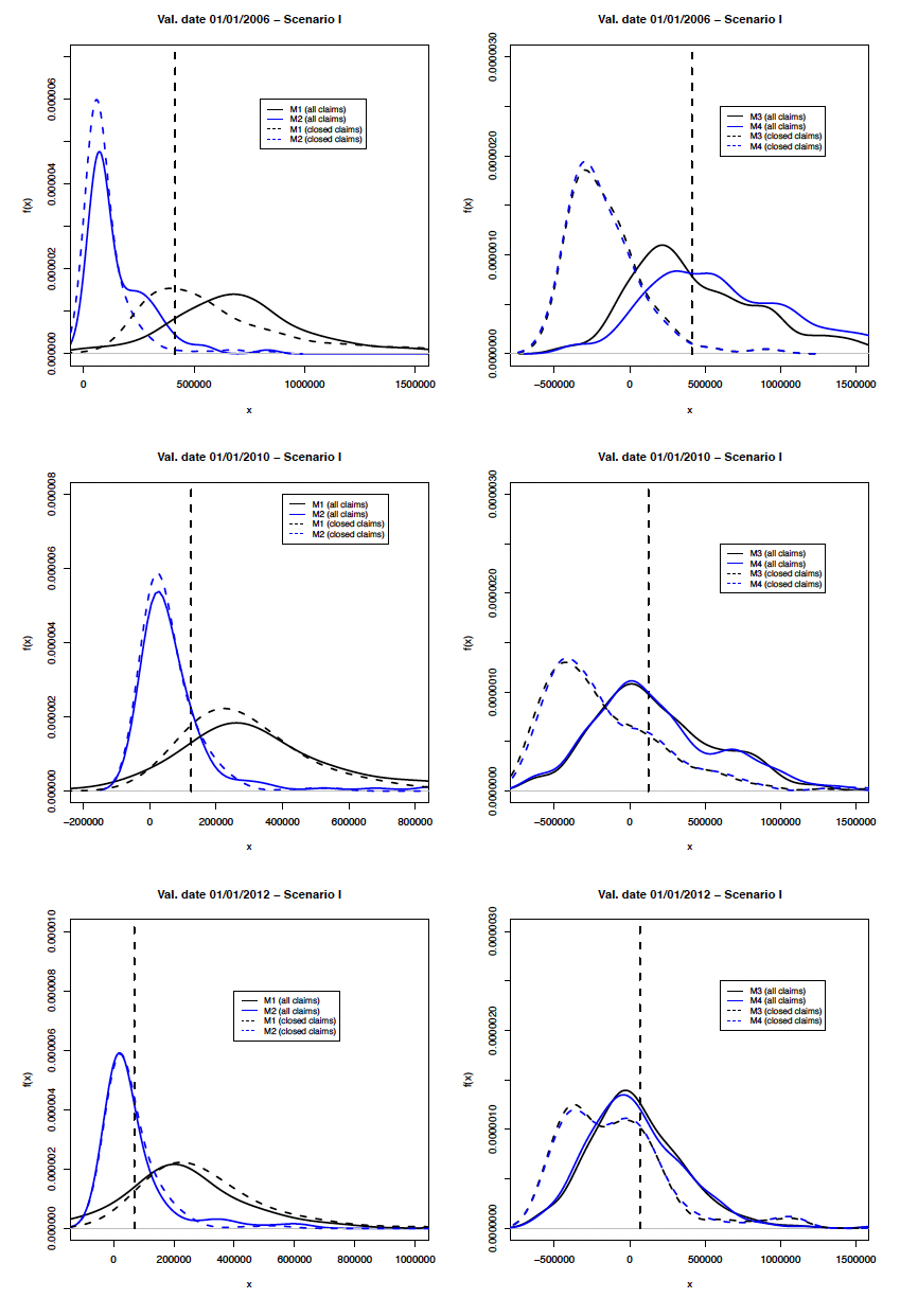
Table 4, Table 6 and Table 8 present the expected values of the reserves using Tree $\widehat{M}_i^{(1)}$, Tree $\widehat{M}_i^{(2)}$, Tree $\widehat{M}_i^{(3)}$ and Tree $\widehat{M}_i^{(4)}$ models for $3$ levels of portfolio maturity: 01/01/2006, 01/01/2010 and 01/01/2012. It is much more informative to look at the predictive distributions of the reserves, which are illustrated in Figure 6. Remember that the most recent occurrence year is 2005; therefore, for the subsequent valuation dates, there is no new claim after December 31, 2005. Figure 6 presents the predictive distributions for the total reserve, IBNR, and RBNS, because, with the collective models, it is impossible to separate the two types of the reserve. For the valuation dates 01/01/2010 and 01/01/2012, this is not a problem since there is no longer an IBNR claim in the database. For the valuation date 01/01/2006, we added the true observed value of the IBNR reserve to the simulated values of the RBNS reserve for Tree $\widehat{M}_i^{(1)}$, Tree $\widehat{M}_i^{(2)}$, Tree $\widehat{M}_i^{(3)}$ and Tree $\widehat{M}_i^{(4)}$ models (similar to what is done in Duval and Pigeon 2019). Because the IBNR reserve ($\$8,000$) is a tiny part of the total reserve ($\$414,000$), the impact on the analysis is negligible. Of course, suppose IBNR represents a significant part of the total amount of the reserve. In that case, comparing the results based on individual approaches with those based on collective approaches will then be strongly biased. For example, this bias can be corrected in an analysis by subtracting the amount actually paid for IBNR claims from the total amount of the reserve obtained from a collective approach (see Duval and Pigeon 2019 for an example). Alternatively, one can complete the individual approach with a simple model for the frequency and severity of IBNR claims (e.g., see Wüthrich 2018 and Baudry and Robert 2019).

In order to determine if the integration of open claims improves the results of the methods tested, we present in Figure 7 predictive distributions of the reserve amount using all claims and only closed claims in the calibration process. In practically all cases, not considering the open files in the calibration process leads to underestimating the risk. This underestimation is particularly important for estimators based on Tree $\widehat{M}_i^{(3)}$ and Tree $\widehat{M}_i^{(4)}$. In addition, this conclusion is similar to that obtained following the analysis made in Duval and Pigeon (2019). Therefore, a simplistic strategy in which open files would be removed from the calibration process is not advisable.

Scenario II: 2 lines of business with no inflation. We construct a validation dataset containing $1,063$ claims, $1,063 \times 12 = 12,756$ annual photographs and accident years between 1994 and 2005. This dataset assumes two lines of business, $LoB$ $1$ and $2$, and no inflation for frequency. We present some descriptive statistics in Table 12 and Figure 12 in Appendix C, as well as in Table 5. Selected values are $\widehat{q}^{(2006, 3)} = 0.80$, $\widehat{q}^{(2006, 4)} = 0.30$, $\widehat{q}^{(2010, 3)} = 0.95$, $\widehat{q}^{(2010, 4)} = 0.95$, $\widehat{q}^{(2012, 3)} = 0.95$ and $\widehat{q}^{(2012, 4)} = 0.9$.

We present results in Table 6. Figure 8 presents the predictive distribution of the reserve amount using all models for the same $3$ levels of portfolio maturity.

Scenario III: 2 lines of business with inflation (frequency). We construct a validation dataset containing $1,060$ claims, $1,060 \times 12 = 12,720$ annual photographs and accident years between 1994 and 2005. This dataset assumes two lines of business, $LoB$ $1$ and $2$, and an inflation rate of $5\%$/year for frequency. We present some descriptive statistics in Table 12 and Figure 12 in Appendix C and in Table 7. Selected values are $\widehat{q}^{(2006, 3)} = 0.8$, $\widehat{q}^{(2006, 4)} = 0.4$, $\widehat{q}^{(2010, 3)} = 0.9$, $\widehat{q}^{(2010, 4)} = 0.9$, $\widehat{q}^{(2012, 3)} = 0.95$ and $\widehat{q}^{(2012, 4)} = 0.95$.

We present results in Table 8. Figure 9 presents the predictive distribution of the reserve amount using all models for the same $3$ levels of portfolio maturity.

For all scenarios, we note that the Tree $\widehat{M}_i^{(1)}$ model (blue line) produces very variable reserves resulting in very high expected values and significantly flattened predictive distributions. This instability is explained by the structure of the estimator, which suffers from the lack of data related to the estimation of $\mathbb{I}\left(M > m, Y > z\right)$. This effect is less pronounced for a more mature portfolio because fewer open claims exist. The Tree $\widehat{M}_i^{(2)}$ model (red line) is much more stable, which is because there is more data to estimate $\mathbb{I}\left(Y > z\right)$ than $\mathbb{I}\left(M > m, Y > z\right)$, and that $Y$ is a variable generally less dispersed than $M$. This conclusion confirms that made in a study (Lopez and Milhaud 2021) which, among these two estimators, suggests “… we recommend to use the strategy (B)a) [Tree $\widehat{M}_i^{(2)}$ model] to make the reserve predictions, as it outperforms all other methods and shows stable results in terms of prediction error….”

In all situations, estimators $\widehat{M}_i^{(3)}$ and $\widehat{M}_i^{(4)}$ offer similar performance, which seems to indicate that the use of individual explanatory variables when imputing missing values does not significantly improve the performance of the model. We still add a caveat to this remark due to the small number of micro-level covariates in the database. Furthermore, estimators $\widehat{M}_i^{(3)}$ and $\widehat{M}_i^{(4)}$ require much shorter computation times than estimators $\widehat{M}_i^{(1)}$ and $\widehat{M}_i^{(2)}$. For scenarios II and III, although Tree $\widehat{M}_i^{(2)}$, Tree $\widehat{M}_i^{(3)}$ and Tree $\widehat{M}_i^{(4)}$ models seem appropriate (see Figures 8 and 9), we would recommend the use of Tree $\widehat{M}_i^{(3)}$ model for its simplicity and its saving in computation time.

As a concluding remark, for some scenarios and some estimators, the expected values for the reserve are sometimes far from the observed values. However, for all three scenarios, the observed value is always within the range of plausible values. Moreover, we notice a skewed predictive distribution in several cases (for example, scenario III), resulting in an empirical median consistently lower than the empirical mean. Thus, the latter is strongly impacted by the slightly more extreme cases observed in the distribution’s right tail.

5. Conclusion

The main objective of this paper is to analyze how open claims should be integrated into an individual reserve valuation process when tree-based approaches are used. We provide a detailed literature review to establish the state-of-the-art regarding tree-based techniques in a loss reserving context. We then pursue a more detailed analysis of two tree-based methodologies proposed to include open files within the valuation of reserves process. More precisely, we present and discuss the approach of Lopez, Milhaud, and Thérond (2016, 2019) using corrective weights based on survival analysis and the one of Duval and Pigeon (2019) using missing data imputation.

With simulated databases obtained using Gabrielli and Wüthrich’s simulation machine and for three different scenarios, we compare the performance of these two methodologies and two classical collective loss reserving strategies. From this case study, we take away the following elements:

• strategy in which open files would be removed from the calibration process is not advisable;

• the two estimators ($\widehat{M}_{i}^{(1)}$ and $\widehat{M}_{i}^{(2)}$) proposed in Lopez, Milhaud, and Thérond (2016, 2019) behave quite differently in all scenarios. The estimator $\widehat{M}_{i}^{(2)}$ should be preferred given the stability it has shown compared to $\widehat{M}_{i}^{(1)}$ which varies greatly;

• the performance of the estimators ($\widehat{M}_{i}^{(3)}$ and $\widehat{M}_{i}^{(4)}$) based on Duval and Pigeon (2019) is rather similar in the three scenarios, indicating that the individual information embedded in the covariates used in the imputation of missing data does not guide the model to better results;

• the two estimators ($\widehat{M}_{i}^{(3)}$ and $\widehat{M}_{i}^{(4)}$) outperform the ones of Lopez, Milhaud, and Thérond (2016, 2019) based on Kaplan-Meier weights regarding computation time.

In future work, it would be interesting to reproduce this analysis using a database with more covariates; some could be dynamic.

---

Acknowledgments

We thank the anonymous reviewers and the associate editor for thoughtful suggestions that improved the original manuscript. Support from the CAS Committee on Knowledge Extension Research is gratefully acknowledged.