Pricing Cyber Risk Insurance Coverages by Means of Epidemic Models and Network Theory

undefined

1. Introduction

In an era dominated by interconnected technologies and digital dependence, the prominence of cyber risk has soared, fundamentally altering the fabric of modern society. This emergent threat not only pervades our daily lives but also poses multifaceted challenges, reshaping how we navigate security, privacy, and the very essence of our societal structures. The expanding reach of cyber vulnerabilities touches every sector, influencing businesses, governments, individuals, and critical infrastructures, which highlights the imperative need for robust strategies to mitigate and adapt to this dynamic risk landscape.

Consequently, it is imperative to structure our operations resiliently, to allow our organizations to weather such assaults with minimal damage and to ensure continuity amid compromised IT frameworks. This resilience—which involves swift detection and halting attacks, mitigating their fallout, rectifying breaches, and securing financial stability through insurance coverage—defines our ability to endure and thrive in the face of adversity (see, e.g., Dacorogna and Kratz 2022). In navigating this intricate landscape of cyber risk, balancing investment in security and resilience emerges as a relevant challenge for management.

In this landscape, precisely defining and conceptualizing cyber risk is a pivotal challenge. The body of literature addressing cyber risk has burgeoned over time, with each work offering nuanced interpretations (World Economic Forum 2012; Böhme and Kataria 2006; Strupczewski 2021), thereby contributing to a diverse array of definitions. Clarifying the concept of cyber risk is essential to understanding its multifaceted nature and implications. Notably, Strupczewski (2021) comprehensively defined cyber risk as: ‘’[An] operational risk associated with performance of activities in the cyberspace, threatening information assets, ICT resources and technological assets, which may cause material damage to tangible and intangible assets of an organisation, business interruption, or reputational harm. The term cyber risk also includes physical threats to the ICT resources within [the] organisation.‘’

To further elucidate this concept, it is helpful to compare other definitions in the literature. For instance, the World Economic Forum (2012) emphasizes the strategic impact of cyber risk, describing it as a threat to business continuity and organizational stability, with a focus on economic and reputational damage. Conversely, Böhme and Kataria (2006) offer a more technical perspective, framing cyber risk primarily in terms of vulnerabilities and threats to information systems, often focusing on the likelihood and potential impact of specific cyber threats. Strupczewski’s (2021) definition is notable for its broad scope, encompassing not only operational risks and performance issues but also physical threats to ICT resources, which is less emphasized in the other definitions. This comprehensive approach addresses both direct and indirect impacts of cyber risks, providing a more holistic view compared with the more narrowly focused perspectives of the other authors.

On the insurance front, quantifying cyber risk is challenging because of its extensive impact on intangible assets, such as data and reputation, making it difficult to evaluate losses. Moreover, the insurability of this risk and the potential for systemic failures (linked to extreme events) present additional complexities for managing cyber risk (see, e.g., Dacorogna and Kratz 2022; Eling and Wirfs 2019; Ai and Wang 2023.

With IT pervading all human activities, interdisciplinary research aims to comprehensively understand cyber risk from various angles (see Awiszus et al. 2021; Xie, Lee, and Eling 2020; and Dacorogna and Kratz 2023, for comprehensive surveys on this subject). As highlighted by Dacorogna and Kratz (2023), traditional actuarial techniques are inadequate for rating and controlling risk accumulation, owing to limited availability of historical data and the need to move beyond past loss records. These issues led researchers to identify five potential model types: actuarial models based on loss data, stochastic models for risk contagion, data-driven artificial intelligence (AI) models, exposure models, and game-theory based models. This discussion centers on stochastic models for risk contagion within networks.

Cyber risk’s distinct characteristic is that it occurs within a vast network of computers and connections, making it conducive to network (or graph) modeling, epidemiological/pandemic modeling, or other appropriate stochastic models. Chen and Hon Keung (2024) developed a modified Wiener process model for the degeneration of network functionality. The susceptible-infectious-susceptible (SIS) epidemic Markov model has been applied to cyber insurance (Fahrenwaldt, Weber, and Weske 2018), and Xu and Hua (2019) explored a modified $\epsilon$-SIS model based on Van Mieghem and Cator’s (2012) proposal. Additionally, Antonio, Indratno, and Simanjuntak (2021) delved into the heterogeneous generalized susceptible-infectious-susceptible (HG-SIS) model (see also, Ottaviano et al. 2018, 2019).

Following these methodologies, we introduce a novel approach that draws on the advancements of Xu and Hua (2019) and Antonio, Indratno, and Simanjuntak (2021), enabling separate modeling of critical and noncritical nodes. The method captures the network’s node heterogeneity and considers the distinct characteristics of critical and standard nodes. This differentiation is pivotal, providing a nuanced understanding of vulnerabilities, which facilitates targeted fortification of critical nodes while optimizing resources to uphold the overall network resilience against potential threats. Indeed, our proposed approach offers a versatile framework that extends its applicability to effectively model whaling phishing scenarios.^[1] By introducing nodes that possess the distinctive trait of more easily infecting nodes with which they are connected,^[2] this method accommodates modeling of such targeted attacks within the network. These specialized nodes significantly elevate the system’s susceptibility to risks, amplifying the potential dynamics of infection beyond the conventional homogeneous node assumption.

Emphasizing the significance of departing from homogeneous node considerations, our methodology not only distinguishes between critical and noncritical nodes but also acknowledges the inherent heterogeneity within the network. This nuanced perspective both enhances the understanding of vulnerabilities and facilitates precise fortification strategies targeting critical nodes. Simultaneously, it optimizes resource allocation, bolstering the network’s overall resilience against a spectrum of potential threats, including sophisticated whaling phishing tactics.

We developed a numerical analysis to evaluate our proposed approach using a simulated network that mirrors the structure of a small- to medium-sized enterprise. Additionally, we conducted sensitivity analyses to assess how variations in the network’s topology and infection dynamics influence the outcomes.

The remainder of this paper is organized as follows: Section 2 introduces foundational concepts of graph theory. Section 3 details our proposed methodology, beginning with the general framework in Section 3.1. Section 3.2 delves into employing epidemiological models for cyber risk, outlining our methodology for identifying infected nodes and assessing claim counts. Cost and recovery functions are discussed in Section 3.3, while Section 3.4 elucidates the simulation algorithm. Computation of premiums is addressed in Section 3.5. Our numerical analysis and ensuing discussions are presented in Section 4. Conclusions follow in Section 5. Appendices summarize the algorithm and main R codes used in the procedure.

2. Preliminaries on graph theory

The study of networks is a multidisciplinary field that amalgamates concepts from mathematics, physics, biology, computer science, social science, and various other domains. Across these disciplines, researchers have developed a diverse toolkit, including mathematical, computational, and statistical methods to analyze, model, and fully comprehend networks. Networks serve as a versatile representation for numerous systems and help to capture intricate connection patterns between components.

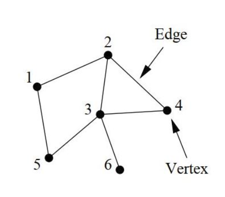
The notion of a network is inherently straightforward: it consists of interconnected points linked by edges. The exploration of networks falls under the purview of graph theory, where graphs serve as the mathematical abstraction of networks (for details, refer to works by Estrada 2011; Harary 1969; Newman 2010).

A network is typically denoted as $G(V,E)$, described as a pair of sets $(V,E)$, where $V=\left\{ 1,...,n\right\}$ is the set of $n$ nodes (or vertices) and $E$ is the set of $m$ edges (or links) represented by points and lines, respectively, in Figure 1. We consider graphs with fixed order $\left\vert V\right\vert =n$ and fixed size $\left\vert E\right\vert =m.$ The edge connecting vertices $i$ and $j$ are denoted by $e_{ij}$. When two vertices share an edge, they are called adjacent.

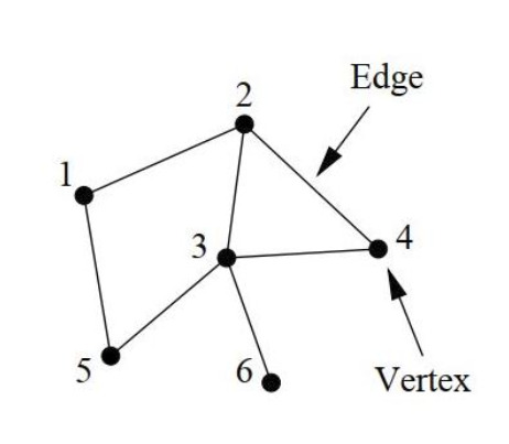
An $n \times n$ nonnegative matrix, denoted as $\mathbf{A}$, characterizes the interconnections between vertices within the graph $G$ and is termed the adjacency matrix. This matrix $\mathbf{A}$ for a simple graph comprises elements $a_{ij}$ defined as follows:

$$a_{ij}=\left\{ \begin{array}{ccc} 1 & \text{if there is an edge between vertices $i$ and $j$} \\ 0 & \text{otherwise} \end{array}. \right.$$

In certain scenarios, assigning a numerical value (often a real number) to edges proves beneficial. Consequently, a weight $w_{ij}$ can be allocated to each edge $e_{ij}$, resulting in a representation known as a weighted graph. In this case, we associate a weighted adjacency matrix $\mathbf{W}$ to the graph. In the context of the weighted adjacency matrix, instead of binary entries indicating the presence or absence of edges between vertices as in the standard adjacency matrix, the entries $w_{ij}$ represent the weights associated with the edges (i.e., the weight of the edge connecting vertices $i$ and $j$).

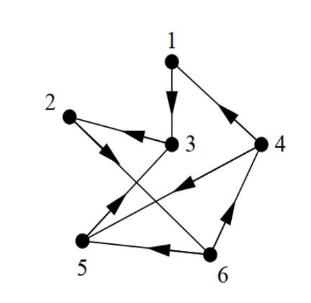
A directed graph (or digraph) represents a type of graph where each edge, referred to as an arc, possesses a direction, indicating a unidirectional link between vertices as depicted in Figure 2. Precisely, every edge in a directed graph is an ordered pair of vertices, delineating a specific flow or connection from one vertex to another.

Notably, the adjacency matrix $\mathbf{A}$ (and $\mathbf{W}$ if the graph is weighted) of a directed graph may exhibit asymmetry due to the directed nature of its edges. This asymmetry distinguishes it from the symmetric nature of adjacency matrices in undirected graphs, reflecting the directional relationship between vertices in the graph.

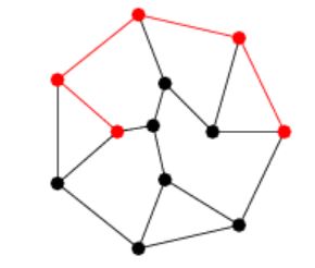
In a network, a path denotes any sequence of vertices wherein each consecutive pair of vertices in the sequence is connected by an edge in the network, akin to the red path depicted in Figure 3. Specifically, an $i-j$ path signifies a sequence of distinct adjacent vertices traversed from vertex $i$ to vertex $j$.

The length of a path refers to the count of edges traversed along the path. A shortest path, also known as a geodesic path, represents the shortest route between two vertices where no other path is shorter. In weighted graphs, the weighted shortest path is the one with the minimum sum of edge weights. The distance $d(i,j)$ between vertices $i$ and $j$ indicates the length of the shortest path connecting them, if such a path exists, and is set to $+\infty$ otherwise.

A graph $G$ is connected if there is a path between every couple of vertices. A graph $G$ is complete when every node is connected to every other.

With directed graphs, paths are directed and comprise a sequence of distinct vertices wherein each consecutive pair of nodes in the sequence is connected by a directed edge that follows the directionality of the graph. Specifically, an $i-j$ path in a directed graph signifies a series of vertices, starting from node $i$ and ending at node $j$, such that each node is linked by directed edges in the specified direction. The definitions of length and distance as well as the extension to the weighted case follow as in the case of undirected graphs.

3. Methodology

3.1. Systemic risk modeling for cyber

Unlike the individual and the collective approaches to cyber risk pricing, systemic risk modeling offers a substantially different perspective. The individual and collective models, along with their derivatives, focus on analyzing the combined cost of claims from a pool of companies or policyholders by identifying shared characteristics and reasoning collectively. They primarily adopt a macroscopic viewpoint.

Conversely, the systemic risk model takes an opposite approach by adopting a microscopic perspective. It aims to reproduce the essential and minimal structure of communication within a specific analyzed company. This is achieved by representing it through a weighted and undirected graph, mimicking the communication interactions within the network over the insurance coverage duration. This approach allows for the dynamic simulation of node infections (i.e., devices, laptops, servers, etc.) throughout the policy period.

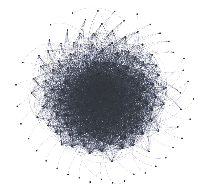
For instance, Figure 4 shows the structure of a network comprising $167$ employees of a manufacturing company.^[3] This network represents internal e-mail communications spanning a period of $9$ months, from January 1, 2010 to September 30, 2010. The data were provided in an anonymized format, and instances where an e-mail had multiple recipients (e.g., To, CC) were documented in separate rows within the dataset. Though not visually represented, the weights in this context denote the communication intensity between different nodes within the company’s communication network. This parameter holds significant relevance in the model, as a higher interaction level between colleagues/nodes correlates with an increased likelihood of vulnerability in case a node is compromised.

It is important to note that acquiring such network data is a challenging task. Some datasets available in the literature are often sourced from e-mail box leaks or made accessible by institutions, such as universities or research entities. Hence, the ability to obtain the network and simulate infection dynamics becomes paramount. Understanding that the internal dynamics of a large multinational company differ from those of a small- or medium-sized enterprise, or a startup with a limited workforce, is crucial. The challenge lies in reconstructing hierarchical structures theoretically, which remains intricate. While relying solely on an e-mail database might be challenging, it can serve as a valuable starting point if accessible to insurers.

3.2. Using an epidemiological model for cybersecurity insurance

Considering the perspective we proposed, we initially focused on a model that considers a company communication network represented as an undirected weighted graph. Its objective is to simulate infections among nodes, both critical and noncritical. When a node is infected, the model simulates the damage incurred and the duration for recovery. Consequently, this simulation aids in determining an insurance premium over the contractual term.

Early studies on infection modeling—for example, Von Neumann’s (1949) work—date back almost a century. Subsequent research in graph theory, computer science, and insurance by various authors (see Awiszus et al. 2023; Märtens et al. 2016; Xu and Hua 2019; Van Mieghem and Cator 2012; Fahrenwaldt, Weber, and Weske 2018), has contributed significantly. Our proposal draws inspiration from Xu and Hua (2019) and Antonio, Indratno, and Simanjuntak (2021) by incorporating specific modifications.

In replicating the infection dynamics during the contractual term it is necessary to consider the status of a node, which can be either infected or secure. A node is infected if it was the victim of an attack in a previous period or if it is still under attack; a node is secure if it is susceptible to an attack. This status needs continual monitoring for each node in the network $G = (V,E)$, with $n$ nodes and $m$ edges, at every time point:

$$\big( I_1(t), \dots, I_n(t) \big), \tag{1}$$

where $I_i(t)$ indicates whether node $i$ is infected ($1$) or secure ($0$) at time $t$.

Another quantity of equal interest is the vector of probabilities of being in a state of infection for each individual node at a certain time $t$:

$$\big( p_1(t), \dots, p_n(t) \big), \quad p_i(t) = \mathbb{P}(I_i(t) = 1). \tag{2}$$

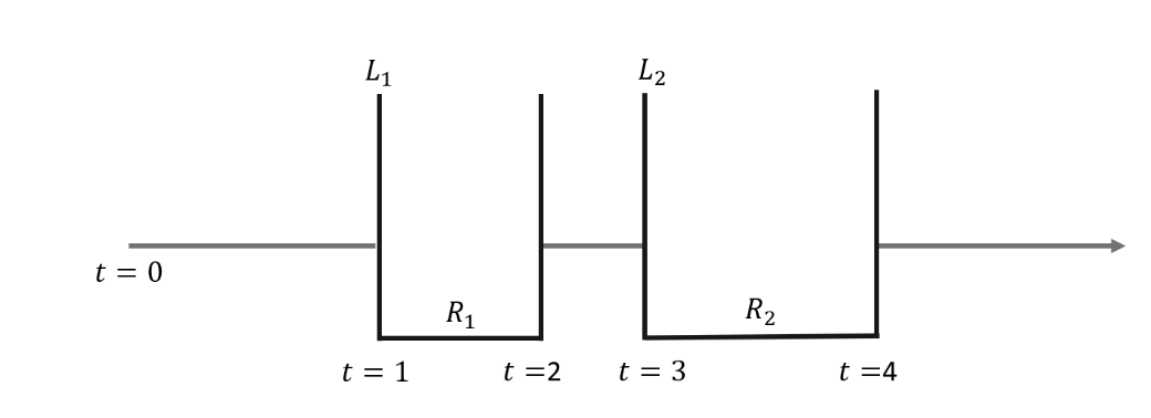
Referencing Figure 5, a node’s infection-recovery scheme portrays its progression. Initially secure, the node becomes infected at $t=1$, incurs a loss $L_1$, undergoes repair with cost $R_1$, and restores functionality by $t=2$. Subsequent infections and recoveries follow a similar pattern.

This infection dynamic is known in the epidemiological literature as the SIS (susceptible, infectious, and susceptible) model, suitable for node infections resulting from the absence of immunity after an infection (see Kermack and McKendrick 1927; Pastor-Satorras and Vespignani 2001). These are compartmental models, so called because the examined population is divided into distinct groups. The SIS model fits very well in the case of node infections since no immunity to subsequent infections is gained.

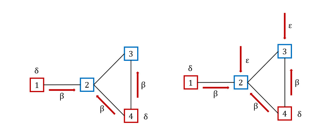
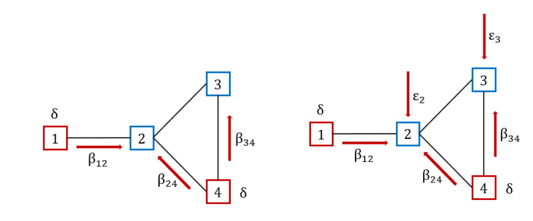
The model, often viewed as a renewal reward process, categorizes the population into distinct groups. It can be seen as a generalization of the Poisson process. In particular, the holding times between events can follow any distribution with finite mean and positive values, not just the exponential distribution. This process is indeed more flexible as it can model a wider variety of real-world phenomena by allowing different distributions for the inter-event times. When the holding times are not exponentially distributed, the process does not have a memoryless property, making it a non-Markov process (see, e.g., Van Mieghem, Omic, and Kooij 2009). This type of model uses two specific parameters, typically denoted with $\beta$ and $\delta$, to describe infection and recovery dynamics, respectively. In particular, as displayed in Figure 6 (left side), in the traditional SIS model, infected nodes, represented in red, can propagate the infection at a rate $\beta$ following existing connections (see, e.g., red arrows connecting nodes 1 to 2, 4 to 2, and 4 to 3) and recover at a rate $\delta$.

In the case where a node can be infected not only by neighboring nodes, but also from outside the network, it is possible to generalize the SIS model by means of an additional parameter $\varepsilon$ (self-infection rate), thus obtaining the $\varepsilon$-SIS model(see, e.g., Van Mieghem and Cator 2012). Figure 6 (right side), illustrates an example where secure nodes 2 and 3 can be infected by neighboring infected nodes at a rate $\beta$, and from outside at a rate $\varepsilon$.

Considering an $\varepsilon$-SIS model, we have for the $i$-th node:

$$\begin{cases} I_i(t):0 \rightarrow 1 \; \text{at rate} \; \beta \sum_{\ell = 1}^n a_{ \ell i}I_\ell(t) + \varepsilon_i \\ I_i(t):1 \rightarrow 0 \; \text{at rate} \; \delta_i \end{cases}, \tag{3}$$

where $a_{\ell i}$ is the $\ell,i$ element of the adjacency matrix associated with the network. Parameters $\beta$, $\varepsilon$, and $\delta$ are not node-specific, which simplifies model complexity. Hence, these models tend to overlook critical aspects, such as network weights, communication intensities among devices, and the presence of different node types in the network (e.g., servers and personal computers).

To address these limitations, we adopted a non-Markov model, known as $HG$-$SIS$ (heterogeneous generalized susceptible-infectious-susceptible), which allows for different $\beta$ values for each arc. At any given moment, the time to infection for a node is determined by the minimum duration among two sets of random variables. The first set comprises the times to infection generated by random variables $Y_{1}, \dots, Y_{D_{i}}$, where $D_i$ represents the infected neighbors of node $i$. Additionally, the node faces a self-infection time denoted by $Z_i$, which accounts for external threats entering the network:

$$T_i = \min \big( Y_1, \dots, Y_i, Z_i \big). \tag{4}$$

This calculation establishes the shortest duration required for a node to succumb to infection, considering both internal risks from infected neighbors and external threats outside the network perimeter.

The HG-SIS model, depicted in Figure 7, potentially involves as many $\beta$ parameters as there are nonzero elements in the adjacency matrix, corresponding to the $m$ arcs. Also, the self-infection and the recovery processes, described by $\varepsilon_{i}$ and $\delta_{i}$, could be different between nodes. As displayed in Figure 7, infected nodes, represented in red, can propagate the infection at different rates through existing connections (see red arrows in the figure), while noninfected nodes are also exposed to different infection probabilities from outside (see $\varepsilon_2$ and $\varepsilon_3$ in the Figure 7.

However, in the case of large networks, this model requires estimating an extensive number of parameters. To address this, we followed the approach of Antonio, Indratno, and Simanjuntak (2021), considering only the values of $\beta$ and $\delta$ and using the edge weights of the network. We employed a sigmoidal transformation to derive the matrix of parameters. The proposed transformation is a function of the weight of the edge considered, values of $\beta$ and $\delta$, and characteristics of the weight distribution. This allowed us to find an $n \times n$ matrix $\mathbf{B}$, whose elements $\beta_{ij}$ are defined as follows:

$$\beta_{ij} = \begin{cases} 0, \quad w_{ij} = 0 \\ \frac{\beta - \delta}{1+exp\left(-\frac{(w_{ij}-\bar{w})}{\sigma}\right)}+ \delta, \quad w_{ij} > 0 \end{cases},\tag{5}$$

where: $$\begin{gathered} \bar{w} = \frac{1}{2 \cdot m}\underset{i,j}{\sum} w_{ij} , \sigma = \frac{\underset{i,j}{\sum} \vert w_{ij} - \bar{w} \vert}{ 2 \cdot m }. \end{gathered}\tag{6}$$

The proposed transformation aims to increase (reduce) the infection probability when the edge weight is higher (lower). This is consistent with the literature that interprets edge weights as communication weights and generally conveys how effectively that edge is transmitting information and infection (see, e.g., Antonio, Indratno, and Simanjuntak 2021; Bartesaghi, Clemente, and Grassi 2024).

Hence, formula (3) becomes

$$\begin{cases} I_i(t):0 \rightarrow 1 \; \text{at rate} \; \sum_{\ell = 1}^n \beta_{\ell i} a_{\ell i}I_\ell(t) + \varepsilon_i \\ I_i(t):1 \rightarrow 0 \; \text{at rate} \; \delta_{i} \end{cases}.\tag{7}$$

In this way, the infection probability between a couple of nodes depends on the weight of the arc connecting the two nodes.

To account for the potential existence of two node types, common or standard nodes and critical nodes, two sets of $\beta$ and $\delta$ are selected. Subsequently, two distinct sigmoidal transformations are applied. This approach aims to create a clearer distinction between parameters, enhancing their impact on infection durations. By implementing this method, we accentuate the differences in infection times between the node types, thereby better reflecting their respective vulnerabilities.

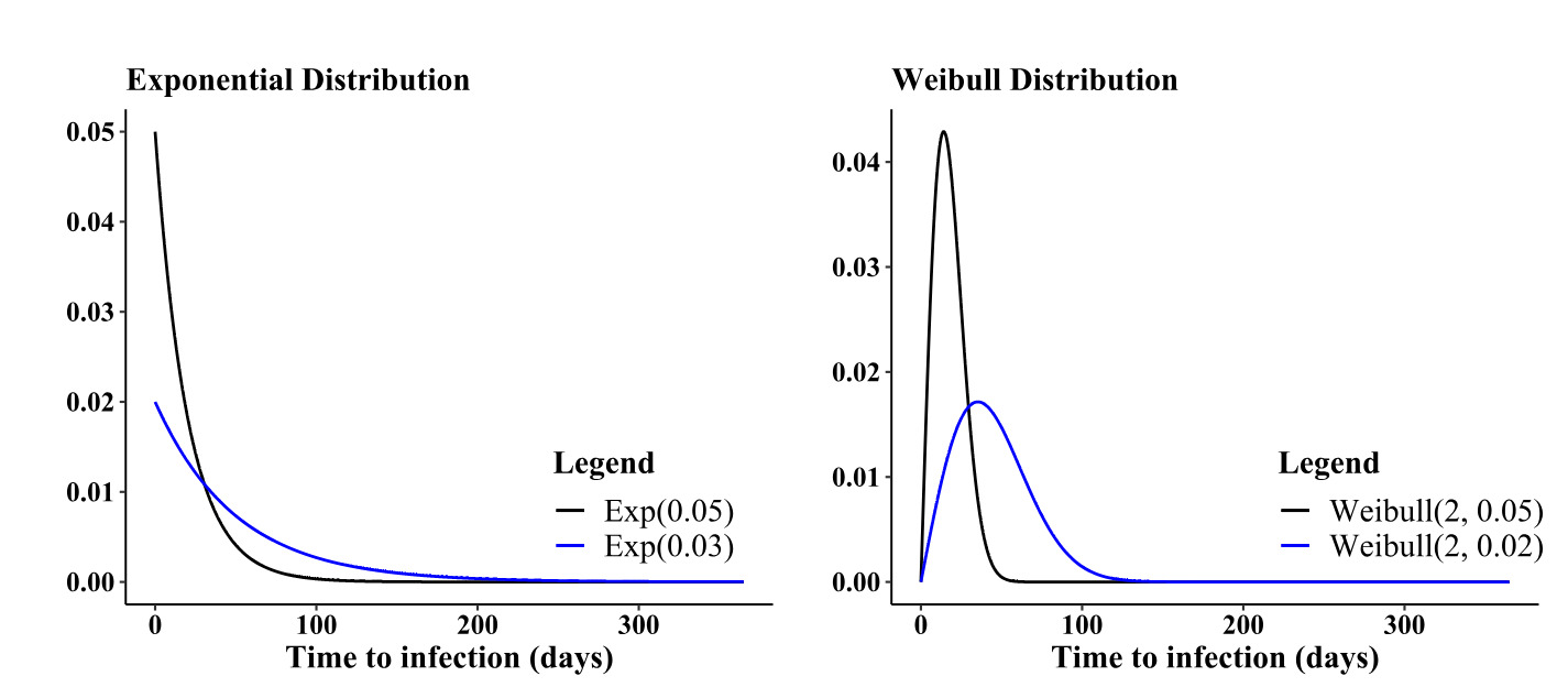
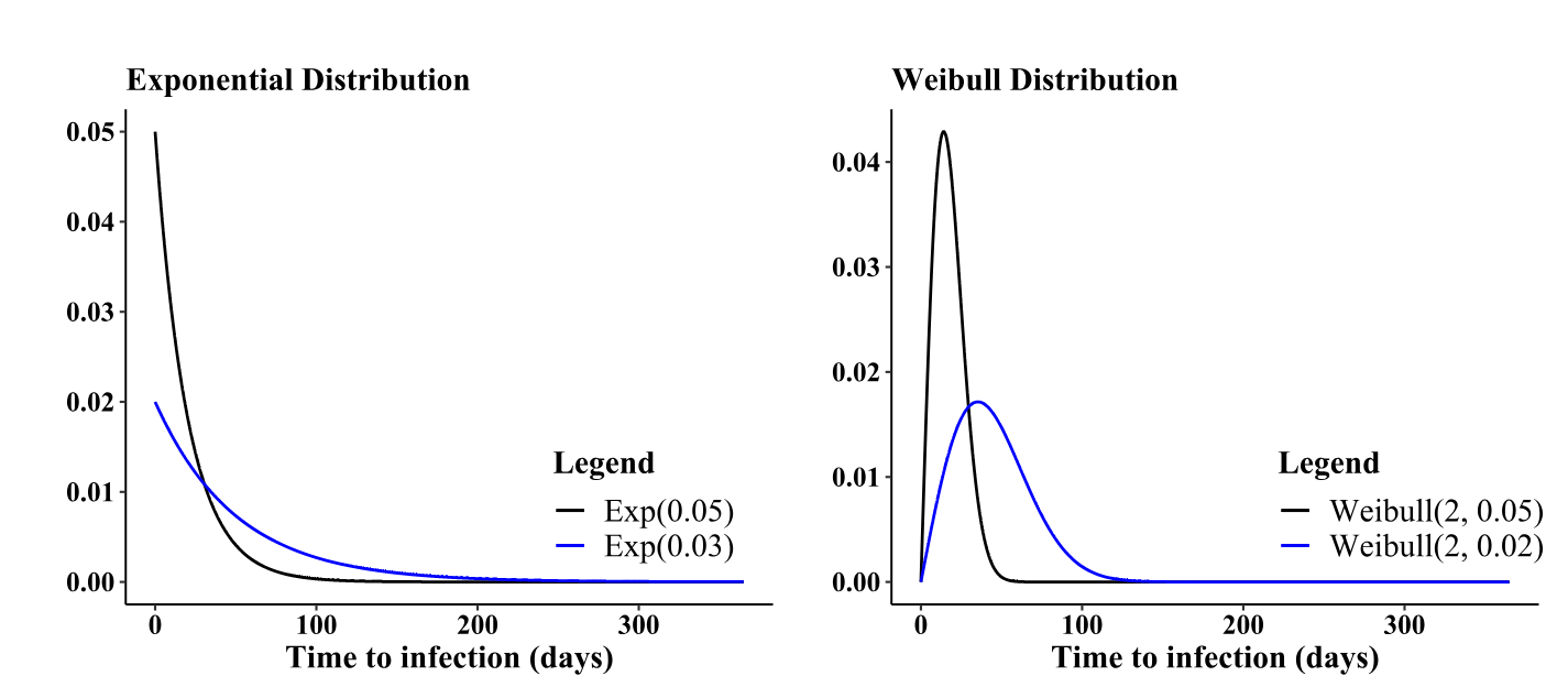
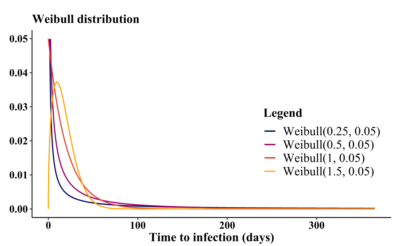
Understanding the advantages of diverse $\beta$ values becomes evident when selecting and fine-tuning distributions to represent infection times. Figure 8 illustrates the behavior of two widely used distributions for infection times concerning parameter adjustments. For instance, observing the exponential distribution, a decrease in $\beta$ results in an increase in the distribution’s mean, consequently extending the infection times. Conversely, the Weibull distribution, unlike the exponential, not only affects the mean, but also allows manipulation of the distribution’s skewness through its shape parameter. Figure 9 depicts the variation in the behavior of the Weibull probability density function as the shape parameter undergoes changes.

In the simulations, we used the Weibull distribution for both time to infection ($\beta$ and $\varepsilon$ parameters) and recovery time ($\delta$ parameter) since it provides greater flexibility. Details of the distribution and connection with parameter $\beta$ are reported in Appendix B. It is worth noting that as $\beta$ increases, both mean and variance tend to zero, while skewness is independent of the parameter $\beta$. From a practical point of view, choosing a very small $\beta$ (or $\delta$ or $\varepsilon$) in the parametrization of the epidemic model will lead to large averages of the times to infection, but consequently also to greater variability in the simulations.

3.3. Cost and recovery functions

After a node becomes infected, it is important to assess the financial implications encompassing both recovery and tangible losses. The critical differentiation lies between critical and noncritical nodes. For the latter, two separate cost functions are established to account for both recovery and loss expenses. Conversely, critical nodes are governed by a singular function. This differentiation arises from the adoption of distinct distributions employed to emulate the incurred damage.

In the scenario where a single node incurs a loss due to infection (or self-infection), it is crucial to model the associated costs. These costs might encompass material damages to the laptop, liabilities incurred toward third parties, economic repercussions resulting from data loss, and more, depending on the contractual terms outlined in the policy. Conversely, concerning the recovery process, the incurred loss refers to the expenses required to restore the node’s functionality.

Cost and recovery function for noncritical nodes

For common nodes, reference is made to the solution adopted by Xu and Hua (2019). The cost function is given by:

$$\eta_i(l_i) = c \cdot l_i, \tag{8}$$

where $l_i$ is simulated using a four-parameter beta distribution. The loss cost function is thus proportional to the loss, according to an appropriately chosen parameter $c$. The beta distribution, on the other hand, is chosen because, for common nodes, it was deemed appropriate to have limited support for the possible realizations of the random variable. When signing a policy, for example, one could insure each simple node in the network up to a value of EUR $1,000–1,500$. In this way, in the event of infection, the loss would be superiorly limited thanks to the use of this beta random variable. Recovery cost function is given by:

$$\rho_i(w_i, r_i) = c_1 \cdot w_i + c_2 \cdot r_i , \tag{9}$$

where $r_i$ is the time required for recovery, modeled by a Weibull distribution, $w_i$ is the initial wealth of the node, and $c_1$ and $c_2$ are two parameters that allow us to amplify or reduce the effect of recovery and initial wealth on the recovery cost. For consistency, the initial wealth of the node could correspond to the upper limit of support within the four-parameter beta distribution.

Figure 10 depicts the histograms of both the loss $l_i$ and the corresponding cost function $\eta_i$. It is evident that by opting for a straightforward cost function, the distribution’s original “shape” and positive skewness remain intact. Similarly, by generating recovery times using a Weibull distribution, we can observe the histogram of the recovery cost function. Once again, the simplicity of the chosen function preserves the initial distribution’s form. In both scenarios, these functions represent basic linear transformations of random variables.

Cost and recovery function for critical nodes

For critical nodes (servers, highly sensitive computers, databases, etc.) we took a different approach concerning claims distribution, diverging from the use of two separate cost functions. The rationale behind this decision stems from the multiple repercussions accompanying the compromise of critical nodes, including not just the device’s damage but also third-party liabilities and potential reputational harm.

Given the presumed resilience and prolonged recovery time of critical nodes compared with common nodes, we selected a lognormal distribution (as in Edwards, Hofmeyr, and Forrest 2016). To account for potential maximum limit effects, a truncated lognormal distribution can also be considered. Additionally, long-tailed distributions, such as Pareto, generalized Pareto, and gamma hold relevance in this context (see Wheatley, Maillart, and Sornette 2016; Sun, Xu, and Zhao 2020). Unlike common nodes—where estimating cost and recovery functions, employing distributions like beta, and calibrating recovery times based on support and IT department resilience is relatively straightforward—critical node estimation poses challenges. While calibrating lognormal distributions proves intricate, a conservative approach permits establishing at least the distribution’s average for pricing purposes. Mean information can be obtained from third-party sources, insurers, or reinsurers, aiding in this estimation process.

3.4. The simulation algorithm

The simulation model we employed is a fusion of a non-Markov model based on Xu and Hua (2019) and an HG-SIS model based on Antonio, Indratno, and Simanjuntak (2021), with an additional improvement to distinguish between critical and noncritical nodes. The objective was to simulate the cumulative loss during the entire time span of the insurance contract (e.g., 1 year). It is possible to assess the cumulative loss $s_i(t)$ of node $i$ at time $t$, calculated by summing the total number $M_i(t)$ of infections of node $i$ up to time $t$, as follows:

$$s_i(t) = \sum_{\ell = 1}^{M_i(t)} \big[ \eta_i(l_{i,\ell}) + \rho_i(w_i,r_{i,\ell}) \big],\tag{10}$$

where $\eta_i$ is the cost function due to infection (or self-infection) (see formula (8) in case of loss, $l_{i,\ell}$, $\rho_i$ is the recovery process function (see formula (9)) depending on initial wealth $w_i$ and the length of the service slowdown $r_{i,\ell}$.

Considering all nodes and summing the cumulative loss up to instant $t$ for all nodes in the network, we obtain the following result:

$$S(t) = \sum_{i=1}^{n} s_i(t) = \sum_{i=1}^{n} \sum_{\ell = 1}^{M_i(t)} \big[ \eta_i(l_{i,\ell}) + \rho_i(w_i,r_{i,\ell}) \big].\tag{11}$$

We summarized the main steps in Algorithm 1, Appendix A, used for quantifying potential losses. The initial step involves the network dataset, containing crucial information, such as node groupings, critical versus noncritical node distinctions, node IDs, and comprehensive node attributes. Following this, defining the number of simulations becomes essential, along with specifying parameters for distributions, including $\beta$, $\delta$, and $\varepsilon$ for critical and noncritical nodes. Additionally, parameters from relevant distributions, distinguishing between critical and noncritical nodes, are necessary to compute infection-related losses and recovery losses.

It is essential to note that, for each secure node, identifying infected neighbors is crucial. By aggregating the $\beta$ parameters corresponding to the examined node’s row and the columns aligned with the IDs of infected neighbors, the infection time can be simulated using a Weibull distribution (including self-infection time). This approach accounts for a dual effect. Consequently, the infection time decreases with a higher weight between a node and its infected neighbors due to the sigmoidal transformation of parameters $\beta$. Moreover, a greater number of infected neighbors leads to a shorter infection time.

Formula (12) exemplifies the summation of betas ($\hat{\beta}_i$), representing the cumulative effect of interconnectedness influencing infection probabilities.

$$\hat{\beta}_i = \sum_{\ell = 1}^{D_i}\beta_{\ell, i}.\tag{12}$$

As depicted in Algorithm 1, the algorithm’s design shows that network topology significantly affects the probability of infection. A more interconnected network increases the likelihood of having infected neighbors, thereby reducing the time to infection for each individual node. Conversely, self-infection times are independent of network topology and depend solely on the calibration of parameters for the chosen distribution.

3.5. Premium calculation

It was mentioned earlier that the aim of Algorithm 1 is to identify the loss cumulated for all nodes in the network. We can define, with the random variable $S(T)$, the total loss at the end of the contract. From a premium calculation perspective, it is essential to identify the risk premium:

$$\mathbb{E}[S(T)].\tag{13}$$

The risk premium is in fact the expected value of the overall compensation to be paid by the insurer over the coverage period. Adding the safety loadings to the risk premium gives the pure premium.

$$P = \mathbb{E}[S(T)] + \text{safety loadings}.\tag{14}$$

This is the global compensation transferred to the insurer. Safety loadings are widely used in actuarial and pricing. They reflect the inherent riskiness of the insurance transaction and are a kind of risk premium but also reflect the remuneration of the cost of capital. Safety loading is intrinsically linked to the cost of capital since, given the Solvency II directive, the higher the riskiness of the LoB considered, the higher the capital requirement and thus the higher the safety loading. In the following simulations, only the risk premium and the pure premium are calculated.

Two approaches are used to calculate the pure premium. The first is the standard deviation principle:

$$P = \mathbb{E}[S(T)] + \alpha \cdot \sqrt{\sigma^2(S(T))}.\tag{15}$$

Basically, the remuneration for risk is proportional ($\alpha$) to the standard deviation of the total cost of claims random variable during the policy coverage period. A second approach is to consider a given percentile (e.g., 60–70th) of the total claims cost distribution, also implicitly considering the skewness of the distribution.

4. A numerical application

As mentioned in Section 3.1, obtaining the company’s communication network data poses significant challenges. Consequently, we have developed an R function that allows us to create an undirected weighted network with specific a priori characteristics. The function is detailed in Appendix C. Subsequently, we transformed the previously acquired network into a weighted one, following the procedure outlined in Appendix C. This section presents and discusses an initial case study and a sensitivity analysis in which some parameters have been varied.

4.1. Initial case study

Data and parameters

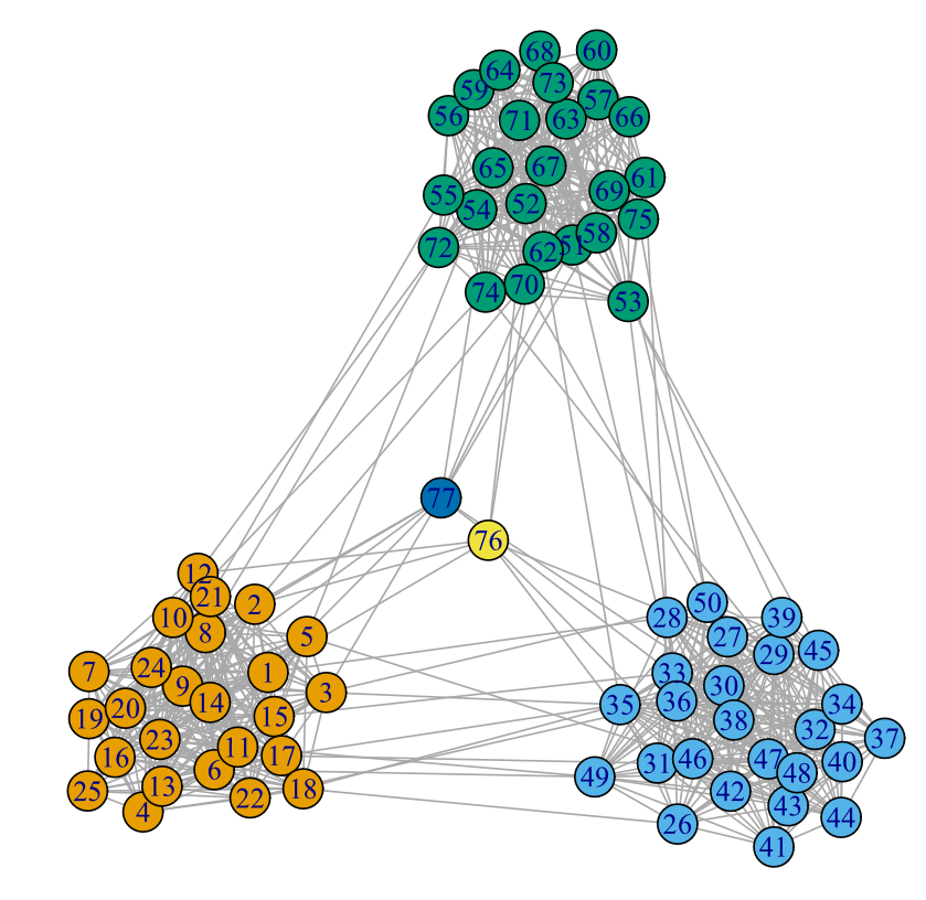
The first network, depicted in Figure 11, comprises $77$ nodes, $75$ of which are common and the remaining $2$ are critical. This network was generated using the R function^[4] described in Appendix C, employing the parameters reported in Table 1.

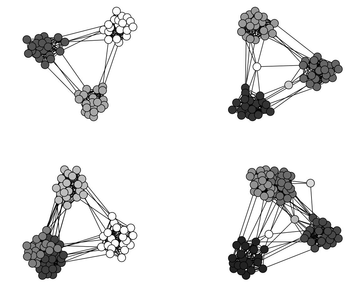
As detailed in Appendix C, this procedure involves a combination of Erdős-Rényi (ER) graphs (Erdős and Rényi 1959, 1960) to create a graph containing distinct nodes, both critical and noncritical. Additionally, we assumed that the connection intensity within a group exceeds that between groups. Moreover, critical nodes exhibit minimal interconnection with other nodes.

Following the steps outlined in Appendix C we assigned weights to the graph’s edges. We made an arbitrary assumption of $20$ communications per node per day on average. However, it is important to note that the minimum weight of an edge is one, and only a small subset of edges carries a high volume of communications during the contract term because of the pronounced positive skewness of the selected distribution.

Starting from this undirected and weighted network, it is possible to set (and calculate) parameters essential for the infection dynamics. These include the maximum and minimum values of $\beta$ for critical and not critical nodes, as well as the required $\alpha$ and $\delta$ values. Using the network weights and the sigmoidal transformation discussed in Section 3.2, all $\beta$ parameter values can be derived. We used the starting parameters in Table 2 for this case study. Consistent with what has been stated so far, the parameters for critical infrastructures are smaller and therefore imply longer times to infection and self-infection than for normal nodes. In addition, the times to recovery and to reestablish node functionality are also longer.

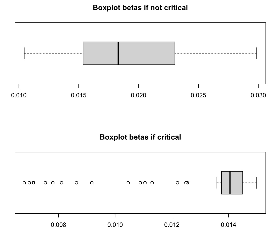
The boxplots illustrating the beta parameters obtained for critical and not critical nodes are presented in Figure 12. These plots showcase the distinctive attributes of the sigmoidal transformation. Positioned between defined minimum and maximum values, these parameters exhibit variability based on the edge weights, which signify the estimated connection intensity during the policy period.

To conduct the simulations, we established the cost and recovery functions for the common nodes as follows: $$\begin{gathered} \eta_i\left(l_i\right)=0.5 \cdot l_i \\ \rho_i\left(w_i, r_i\right)=0.2 \cdot 1000 + 2 \cdot r_i \end{gathered}.$$

Here, each node begins with an initial wealth of EUR $1,000$, and a four-parameter beta distribution characterizes the severity of the loss. However, for critical nodes, we selected a singular cost/recovery function. In the event of infection in a critical node, the cost of damages, encompassing losses to third parties and physical assets, is determined from a truncated lognormal distribution, which accounts for the expenses required to restore the critical infrastructure to its full operational state. This choice stems from the typical existence of maximum limits in insurance contracts for such damages and the significant tail end of the distribution.

Simulation results

After obtaining the initial graph and gathering all required parameters, we executed Algorithm 1 from Section 3.4; the results are detailed below.

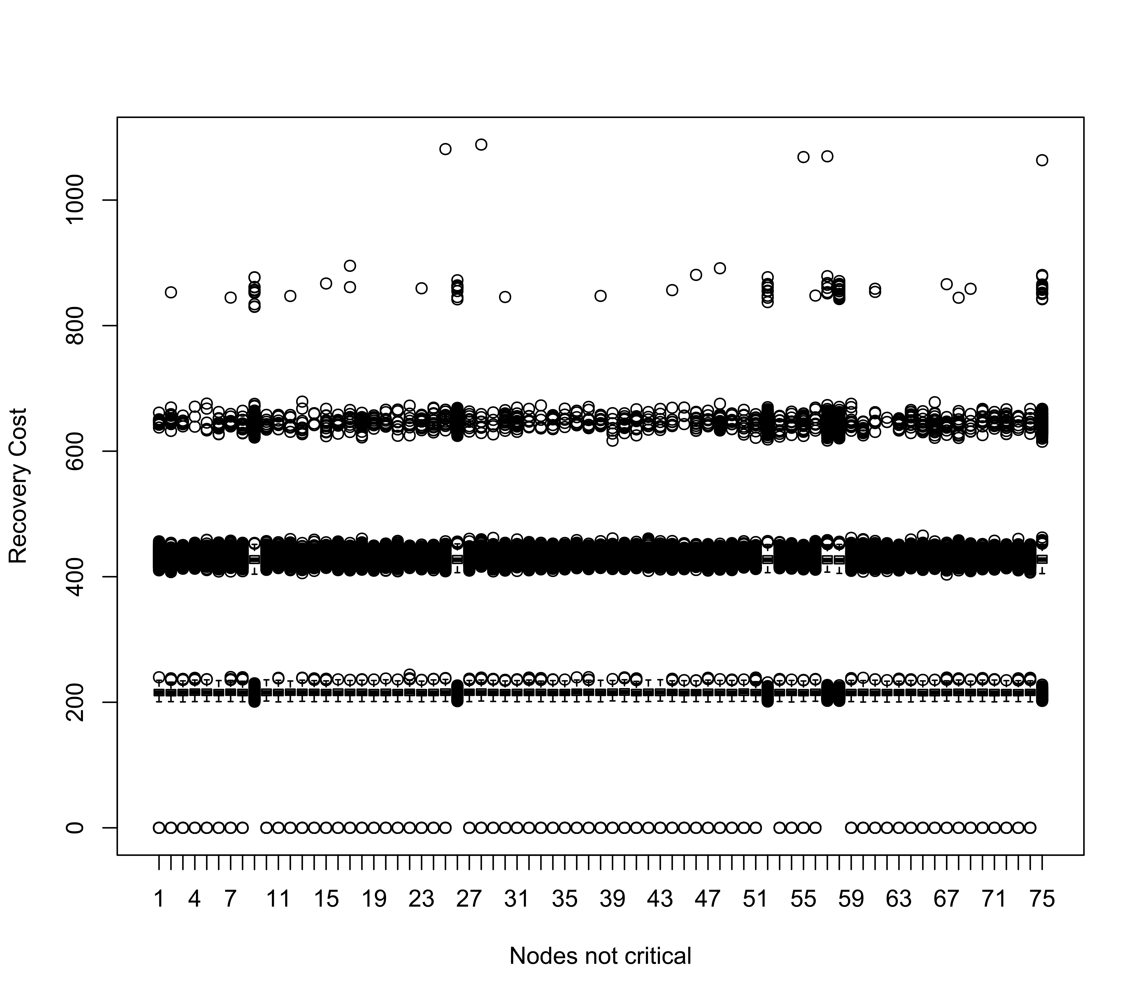
Figure 13 displays the boxplots illustrating the incurred loss costs solely for not critical nodes. These plots showcase a consistent behavior, highlighting multiple infections of individual nodes during the policy period. Similarly, Figure 14 portrays the recovery cost boxplots. Since the recovery cost is contingent on the duration needed for recovery, a discernible pattern emerges, reflecting repeated infections of the same nodes.

The loss/recovery boxplots for critical nodes are depicted in Figure 15. The substantial impact of critical nodes on the aggregated cost of claim distribution is evident owing to their heightened severity compared with common nodes. Additionally, note that within this framework, prior infection does not confer immunity, potentially escalating the damage for critical nodes.

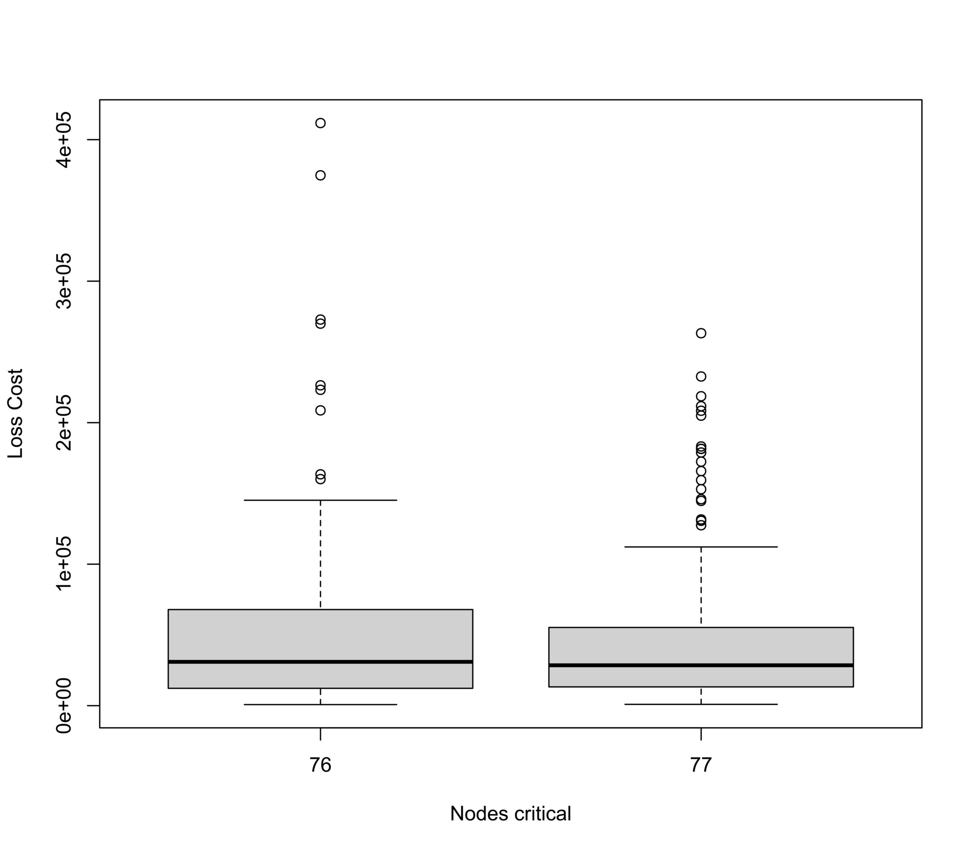
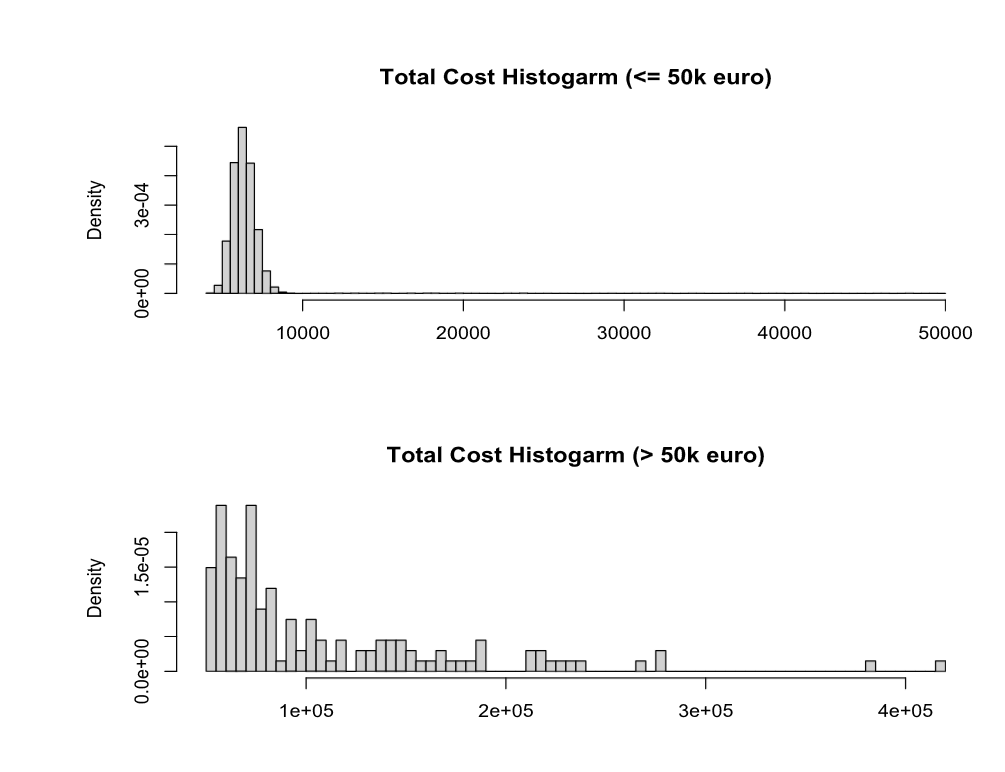
Since the total cost of claims arises from both common and critical node infections, understanding the resultant distribution by amalgamating these source distributions is crucial for insurers. Figure 16 illustrates that while infections among common nodes often result in limited claims, a few critical infrastructures can incur potential losses of up to a half million euros. These striking disparities confirm the significance of our proposed method, which enables the separate modeling of common and critical nodes, offering a more comprehensive insight into potential risks for insurers.

To relate simulation outcomes to a known distribution, we applied Cullen and Frey’s (1999) method. The (nonparametric) bootstrap results in Figure 17 suggest that estimating the total aggregate distribution using a gamma distribution is feasible. To support this evidence, Figure 18 illustrates the contour plot of the combination between skewness and kurtosis.

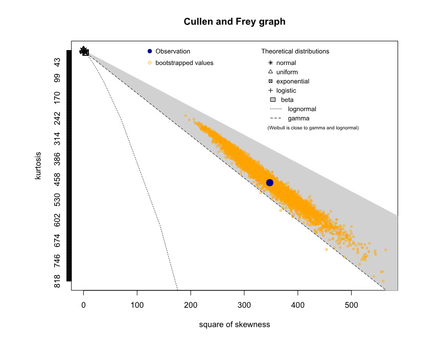
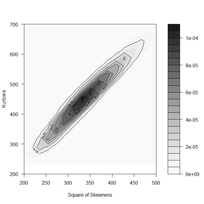
Table 3 presents an overview of the key attributes characterizing the distribution of total losses incurred. The significant impact of two distinct node types affected differently by infection dynamics, coupled with their notably disparate associated costs, is a prominent feature. This convergence manifests in a distribution marked by considerable skewness. The presence of these disparities not only underscores the intricate nature of the infection dynamics but also accentuates the pivotal role played by our modeling approach in capturing these nuances.

These statistics empower insurance companies to precisely calculate the premium. For instance, considering a safety loading assessment at $1\%$ of the standard deviation, the derived premium approximates to around EUR 95 per node.

4.2. Sensitivity analyses

We present here a sensitivity analysis in which certain topological characteristics of the network are primarily altered. As shown in Figure 19, the number of nodes remains constant, while the number of groups has increased (from 3 to 5) and the connection probabilities within and between groups has also increased. Compared with our previous analysis, we kept invariant the number of critical infrastructures and the probability of their connection with common nodes. The aim was to evaluate how an insured firm characterized by different connections could be exposed to cyber risk.

In addition to the increased connections between common nodes, which make the network more prone to greater numbers of infections, the thresholds for beta parameters have also been changed. The new beta parameters, whose distributions are summarized in the boxplot displayed in Figure 20, will therefore vary between 0.04 and 0.02 (with respect to the range observed before, $(0.01,0.03)$). Thus, by means of the sigmoidal transformation, a decrease in the time to infection and, consequently, a higher number of infections is expected. However, it should be noted that varying only the beta parameter does not necessarily imply that there are more (or fewer) infections in the network, because a predominant behavior in the infection dynamics could be driven by the self-infection probability and, more importantly, the network recovery times.

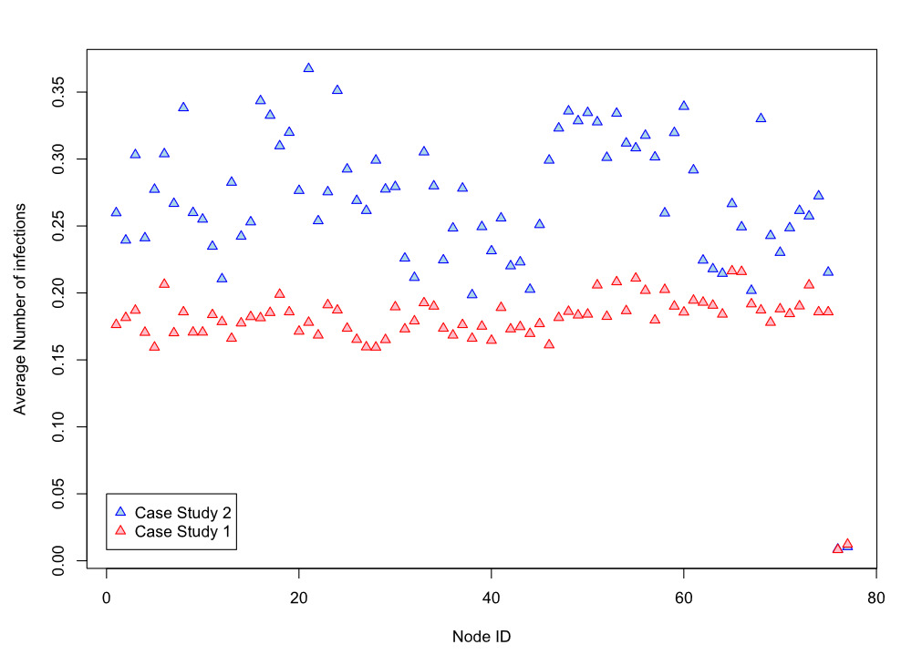
Figure 21 summarizes and highlights the differences with respect to the previous results. It depicts the average number of infections for each node, including the two nodes representing critical infrastructures. It is apparent that the new network, having a different topology from the first and different parametrization of infection times, has a systematically higher average number of infections per node. However, this difference is not appreciable in the case of the critical infrastructures, which did not show a change in the number of interconnections with common nodes. This is an essential aspect to note, as it shows, with a simulative approach, and in this framework, that if well protected, critical infrastructures can be very resilient to cyber attacks.

As also illustrated in Table 4, the risk premium in this case increased significantly ($+17.40\%$). The same trend is also present for the median and the $70th$ percentile of the distribution. Conversely, the standard deviation is smaller than before, probably because of the more homogeneous topology of the network. A more connected network suggests less variability between nodes and thus a lower standard deviation, given the cost functions chosen for this analysis.

Consistent with the methodology adopted above, using a safety loading coefficient equal to 1% of the standard deviation, the resulting premium is about EUR 111 ($\approx$ 17.1% higher).

5. Conclusions

This paper addresses the emerging threat of cyber risk in our digitally dependent era. We emphasize the need for robust strategies to mitigate cyber attacks and to structure our operations resiliently. We provide a comprehensive delineation of cyber risk, including operational risks, threats to information and technological assets, and potential damage. Quantifying cyber risk and evaluating losses is challenging due to the impact on intangible assets. We highlight the interdisciplinary nature of research on cyber risk and discuss different model types, including network and stochastic models. Traditional actuarial techniques are inadequate for rating and controlling risk accumulation; consequently, researchers are identifying more effective model types, including stochastic models for risk contagion.

Cyber risk’s distinct characteristic of occurring within a vast network of computers and connections lends itself to network or graph models, epidemiological/pandemic models, and other stochastic models. We have discussed several existing models, such as the susceptible-infectious-susceptible epidemic Markov model, and introduced our novel approach that considers separate modeling of critical and noncritical nodes in the network. This approach captures the heterogeneity within the network and facilitates targeted fortification of critical nodes while optimizing resources to enhance overall network resilience.

To evaluate our proposed approach, we conducted a numerical analysis using a simulated network mirroring the structure of a small- to medium-sized enterprise and performed sensitivity analyses to assess the impact of network topology variations and infection dynamics on the outcomes. Our approach offers a versatile framework for modeling cyber risk, particularly in scenarios involving targeted attacks, such as whaling phishing. By considering the distinct characteristics of critical and noncritical nodes and acknowledging the heterogeneity within the network, our approach enhances our understanding of vulnerabilities and enables precise fortification strategies. It optimizes resource allocation and strengthens the network’s resilience against various potential threats. Future research in this area should further explore the applicability and effectiveness of our approach in different network structures and real-world settings.

While network models offer valuable insights into the structure and dynamics of cyber risk, there are inherent limitations to their application in cyber risk assessment. Understanding these limitations is crucial for refining our approaches and improving their effectiveness. One key limitation is the complexity of accurately representing and simulating real-world network topologies. Network models often simplify the intricate relationships and interactions within a network, which can lead to oversimplified assumptions about how attacks propagate and impact various nodes. This simplification may result in inaccurate risk assessments or failure to capture critical vulnerabilities. Additionally, network models typically rely on static representations of network structures, whereas real-world networks are highly dynamic and constantly evolving. Changes in network configuration, such as adding or removing nodes and connections, can significantly alter the risk landscape. Static models may not effectively account for these dynamic changes, potentially leading to outdated or incomplete risk evaluations. Another challenge is the difficulty in quantifying and incorporating the impact of intangible assets and complex interdependence within the network. Network models often focus on the structural aspects of cyber risk but may struggle to integrate qualitative factors, such as organizational culture, human behavior, and the nuances of emerging threats. These factors can significantly influence the overall risk and are not always easily captured in network-based approaches. Finally, network models may have a limited ability to address the heterogeneity of nodes within a network. While our proposed approach introduces a distinction between critical and noncritical nodes, many network models treat all nodes as homogeneous entities. This lack of differentiation can overlook important variations in node functions, security measures, and susceptibility to attacks.

As cyber risk continues to evolve in tandem with advancements in technology, future research should increasingly consider the role of artificial intelligence for enhancing cyber risk management and mitigation strategies. Integrating AI could significantly impact various aspects of cyber risk modeling and management, providing new tools and techniques for improving network resilience and response capabilities. One promising avenue for future research is the application of AI-driven analytics to improve cyber threat detection and prediction. Machine learning algorithms, for instance, can analyze vast amounts of network traffic data to identify unusual patterns indicative of potential attacks. By incorporating these AI tools into our proposed framework, researchers can enhance the accuracy of risk assessments and better anticipate potential vulnerabilities within the network. Additionally, AI can contribute to the development of adaptive defense mechanisms that dynamically respond to emerging threats. For example, AI systems could be used to automate the security measures adjustments in real time based on ongoing threat intelligence and network behavior. This capability could be integrated into our novel approach of modeling critical and noncritical nodes, allowing for a more responsive and resilient network defense strategy. Furthermore, AI techniques such as natural language processing could improve phishing detection by analyzing and categorizing communication patterns to identify sophisticated phishing attempts, including whaling phishing. This could augment our framework’s ability to target specific threats more precisely and allocate resources more effectively.

Exploring the potential of AI in the context of cyber risk requires a multidisciplinary approach, combining expertise from cybersecurity, machine learning, and network theory. Future research should focus on developing and validating AI-enhanced models that integrate seamlessly with traditional stochastic and network-based models. It will also be important to assess the effectiveness of these AI-driven approaches in various real-world scenarios and network structures. In conclusion, incorporating AI into cyber risk management represents a significant opportunity to advance our understanding and capabilities in this field. By leveraging AI, future research can develop more sophisticated tools for risk assessment and mitigation, ultimately strengthening network resilience and improving response strategies against evolving cyber threats.

G <- make_a_matrix(num_groups, 
        size_group, 
        p_within, 
        p_between, 
        num_criticals, 
        p_criticals, 
        overlapping, 
        intensity_overlapping, 
        overlapping_quota)