Case Studies Using Credibility and Corrected Adaptively Truncated Likelihood Methods

1. Introduction

Credibility theory is one of the oldest but still most common premium ratemaking techniques in the insurance industry, and it continues to attract the attention of practicing actuaries and academic researchers. Since the publication of the first regression-linked credibility model (Hachemeister 1975), numerous extensions, improvements, and practical applications of this model have been proposed in the actuarial literature. Here is a short but representative list of recent papers on this topic:

• Frees, Young, and Luo (1999) gave a longitudinal data analysis interpretation of the standard (Bühlmann 1967; Bühlmann and Straub 1970) and other additive credibility ratemaking procedures. This interpretation also remains valid in the framework of mixed linear models. A few years later, the same authors presented several case studies involving such models (Frees, Young, and Luo 2001).

• Fellingham, Tolley, and Herzog (2005) analyzed a real data set provided by a major health insurance provider, which summarized claims experience for select health insurance coverages in Illinois and Wisconsin. Credibility methods, in conjunction with mixed linear models and Bayesian hierarchical models, were used to make next-year predictions of claims costs.

• Guszcza (2008) provided an excellent introduction to hierarchical models that can be viewed as an extension of traditional (linear) credibility models. Several hierarchical models were then used in a loss reserving exercise to model loss development across multiple accident years.

• Klinker (2011) introduced generalized linear mixed models (GLMM) as a way of incorporating credibility in a generalized linear model setting. The application of a GLMM to a case study on ISO data revealed connections between this approach and the Bühlmann-Straub credibility.

As is the case with many mathematical models, credibility-type models contain unknown structural parameters (or, in the language of mixed linear models, fixed effects and variance components) that have to be estimated from the data. For statistical inference about fixed effects and variance components, traditional likelihood-based methods such as (restricted) maximum likelihood estimators, (RE)ML, are commonly pursued. However, it is also known that while these methods offer most flexibility and full efficiency at the assumed model, they are extremely sensitive to small deviations from the hypothesized normality of random components as well as to the occurrence of outliers. To obtain more reliable estimators for premium calculation and prediction of future claims, various robust methods have been successfully adapted to credibility theory in the actuarial literature (see, for example, Garrido and Pitselis 2000; Dornheim and Brazauskas 2007; Pitselis 2002, 2008).

At this point a short discussion about robust statistics—a well-established field in statistics—might aid the reader who is not familiar with this area. In a nutshell, robust statistics is concerned with model misspecification (or using the actuarial terminology, model risk) and data quality (e.g., measurement errors, outliers, typos). The main focus is on parametric models, their fitting to the observed data, and identification of outliers. Fitting of the model, however, is accomplished by employing procedures that are designed to have limited sensitivity to changes in the underlying assumptions as well as to “unexpected” data points. The procedures that possess such properties are called robust. A very important tool for measuring performance of and for providing guidance on how to construct robust estimators is the influence function (IF). The IF helps to quantify the estimator’s robustness and efficiency, which usually are two competing criteria. Typically, robust and efficient estimators belong to one of three general classes of statistics: L-, M-, or R-statistics. (Here, L stands for linear in the “linear combinations of order statistics”; M stands for maximum in the “maximum likelihood type statistics”; R stands for ranks in the “statistics based on ranks”.) It is not uncommon, however, to have estimators that can be reformulated within more than one of these classes. On the other hand, despite the existing overlap, each type of these statistics has its own appeal. M-statistics, for example, are arguably the most amenable to generalization and often lead to theoretically optimal procedures. R-statistics can be recast in the context of hypothesis testing and enjoy a close relationship with the broad field of nonparametric statistics. L-statistics are fairly simple computationally and have a straightforward interpretation in terms of quantiles.

Further, in the initial stages of its development, research in the field of robust statistics was focused on quite simple parametric problems (e.g., estimation of the location parameter of a bell-shaped curve), but over the years it expanded into linear models, time series analysis, and other more complex problems. Now, almost five decades later, the impact of robust statistics is felt in numerous applied and interdisciplinary areas, ranging from natural and social sciences to computer science, engineering, insurance, and finance. Robust procedures add the most value to the modeling process when the underlying model contains many unknown parameters and/or multiple assumptions, because the more complex the model, the higher the chance to misspecify it. Finally, robust statistics is parametric by its nature and thus differs from empirical nonparametric methods which have no (or very weak) parametric assumptions. The main advantages the parametric methods enjoy over the nonparametric ones are: (a) parametric models are easier to interpret, (b) they are parsimonious, i.e., have few parameters, and (c) they facilitate inference beyond the range of observed data. On the other hand, the attentive reader will recognize that some of these advantages are also risks (e.g., extrapolation beyond the data). Therefore, in this context, robust techniques are indispensable, since they focus on model risk management. For a comprehensive (and much deeper) introduction into the area of robust statistics, the reader should consult Maronna, Martin, and Yohai (2006). Note also that in the academic literature and actuarial practice there exist various methods that are labeled “robust” or “robust-efficient” but fall outside the scope of the present discussion. For example, quantile regression also has the robustness-efficiency quality, but the estimated variable/parameter is generally not the object of actuarial interest. Another popular approach uses a large loss adjustment before the model fitting, which is supposed to “robustify” the estimation process. This approach, however, has no theoretical justification and thus its statistical properties are unknown.

Let us get back to the robust methods at the intersection of credibility and mixed linear models. In this area, the most recent proposal—corrected adaptively truncated likelihood methods (CATL)—is designed for situations when heavy-tailed claims are approximately log-location-scale distributed (Dornheim and Brazauskas 2011b, 2011a). This new class of robust-efficient credibility estimators enjoys a number of desirable features.

• First, it provides full protection against within-risk outliers and observations that may have disturbing effects on the estimation process of the between-risk variability. (Note that the latter property cannot be guaranteed when one applies standard versions of M-estimators that solely robustify the estimation of the individual’s claim experience.)

• Second, the estimators do not require expert judgment to find appropriate truncation points which are obtained adaptively from the data.

• Third, the CATL procedure automatically identifies and removes atypical data points without employing extensive graphical tools or including data-specific predictor variables into the model. This makes the modeling process easier and quicker. (Note that the emphasis on the automatic nature of CATL methods should not be viewed as the authors’ endorsement of the fact that the decision-making process can now be delegated to computers. Understanding of the practical problem, its context, available data, and the economic consequences of the model-based decisions is the sole province of human intelligence . . . at least in the foreseeable future.)

In this paper, we further explore how the CATL approach can be used for pricing risks. We extend the area of application of standard credibility ratemaking to several well-studied examples from property and casualty insurance, health care, and real estate fields. We do not merely determine prices via CATL but rather walk the reader through the entire process of outlier identification and the associated statistical inference using examples. The featured data sets include exposure measures, heteroscedasticity, random and fixed effect covariates and outliers. Throughout the case studies performance of CATL methods is compared to that of other robust regression credibility procedures.

The rest of the paper is organized as follows. In Section 2, we present the CATL procedure for fitting heavy-tailed mixed linear models and the resulting formulas for robust-efficient credibility premiums. In Section 3, we analyze Hachemeister’s bodily injury data using CATL and compare the findings with those of classical robust methods. For illustrative purposes, we fit a log-normal regression model (although other log-location-scale models could be considered as well) and show how exposure measures are incorporated to account for heteroscedasticity in the data. The impact of a single within-risk outlier on the computation of credibility estimates of future claims as well as their prediction intervals is discussed. The case study of Section 4 is related to health care data that contains Medicare costs for inpatient hospital charges classified by state. This data set is also contaminated by outlying risks and thus offers further insights into how robust procedures act on data. Moreover, we fit a more generic regression-type model that requires additional explanatory variables. Robust credibility estimates and prediction intervals for future Medicare costs are computed and compared to those of classical methods. In Section 5, we venture outside the actuary’s comfort zone and demonstrate the usefulness of CATL procedures in the field of real estate. We analyze a widely studied data set of Green and Malpezzi (2003). Summary is provided in Section 6.

2. CATL credibility for heavy-tailed claims

In Section 2.1, we outline the corrected adaptively truncated likelihood procedure for fitting mixed linear models with heavy-tailed error components. Robust credibility ratemaking is briefly discussed in Section 2.2. More technical details on mixed linear models for heavy-tailed claims is presented in Appendix (Sections 7.2 and 7.3). For a complete description of these methods, see Dornheim (2009).

2.1. The CATL procedure

For robust-efficient fitting of the mixed linear model with normal random components, Dornheim (2009) and Dornheim and Brazauskas (2011b) developed adaptively truncated likelihood methods. Those methods were further generalized to log-location-scale models with symmetric or asymmetric errors and labeled corrected adaptively truncated likelihood methods, CATL (Dornheim 2009; Dornheim and Brazauskas 2011a). More specifically, utilizing the notation of Sections 7.2 and 7.3, the CATL estimators for location λ_i and variance components $\sigma_{\alpha_1}^2, \ldots, \sigma_{\alpha_q}^2, \sigma_{\varepsilon}^2$ can be found by the following three-step procedure:

1. Detection of within-risk outliers.

   Consider the random sample

   $$\begin{aligned} \left(\mathbf{x}_{i 1}, \mathbf{z}_{i 1}, \log \left(y_{i 1}\right), v_{i 1}\right), \ldots,\left(\mathbf{x}_{i_{i} i}, \mathbf{z}_{\pi_{i} i}, \log \left(y_{i_{i} i}\right)\right. & \left., v_{i_{i} i}\right) \\ i & =1, \ldots, I . \end{aligned}$$

   In the first step, the corrected re-weighting mechanism automatically detects and removes outlying events within risks whose standardized residuals computed from initial high breakdown-point estimators exceed some adaptive cutoff value. This threshold value is obtained by comparison of an empirical distribution with a theoretical one. Let us denote the resulting “pre-cleaned” random sample as

   $$\begin{array}{l} \left(\mathbf{x}_{i 1}^{*}, \mathbf{z}_{i 1}^{*}, \log \left(y_{i 1}^{*}\right), v_{i 1}^{*}\right), \ldots,\left(\mathbf{x}_{i i_{i}^{*}}^{*}, \mathbf{z}_{i t i}^{*}, \log \left(y_{i t i}^{*}\right), v_{i t i}^{*}\right), \\ i=1, \ldots, I . \end{array}$$

   Note that for each risk i, the new sample size is $\tau_i^*\left(\tau_i^* \leq \tau_i\right)$.

2. Detection of between-risk outliers.

   In the second step, the procedure searches the pre-cleaned sample (marked with *) and discards entire risks whose risk-specific profile expressed by the random effect significantly deviates from the overall portfolio profile. These risks are identified when their robustified Mahalanobis distance (this is a Wald-type statistic with robustly estimated input variables) exceeds some adaptive cutoff point. The process results in a “cleaned” sample of risks, denoted as

   $$\begin{array}{r} \left(\mathbf{x}_{i 1}^{* *}, \mathbf{z}_{i 1}^{* *}, \log \left(y_{i 1}^{* *}\right), v_{i 1}^{* *}\right), \ldots,\left(\mathbf{x}_{i \tau_{i}^{*}}^{* *}, \mathbf{z}_{i \tau_{i}^{*}}^{* *}, \log \left(y_{i \pi_{i}^{*}}^{* *}\right), v_{i \tau_{i}^{*}}^{* *}\right), \\ i=1, \ldots, I^{*} . \end{array}$$

   Note that the number of remaining risks is I* (I* ≤ I).

3. CATL estimators.

   In the final step, the CATL procedure employs traditional likelihood-based methods, such as (restricted) maximum likelihood, on the cleaned sample and computes re-weighted parameter estimates $\hat{\beta}_{C A T L}$ and $\hat{\theta}_{C A T L}=\left(\hat{\sigma}_{\alpha_1}^2, \ldots, \hat{\sigma}_{\alpha_q}^2, \hat{\sigma}_{\varepsilon}^2\right)$. Here, the subscript CATL emphasizes that the maximum likelihood type estimators are not computed on the original sample, i.e., the starting point of Step 1, but rather on the cleaned sample which is the end result of Step 2.

Using the described procedure, we find the shifted robust best linear unbiased predictor for location:

$$\hat{\lambda}_{i}=\mathbf{X}_{i}^{* *} \hat{\boldsymbol{\beta}}_{c A T L}+\mathbf{Z}_{i}^{* *} \hat{\alpha}_{r B U P, i}+\hat{E}_{F_{0}}\left(\varepsilon_{i}\right), \quad i=1, \ldots, I,$$

where $\hat{\beta}_{C A T L}$ and $\hat{\alpha}_{r B L U P, i}$ are standard likelihood-based estimators but computed on the clean sample from Step 2. Also, $\hat{E}_{F_0}\left(\varepsilon_i\right)$ is the expectation vector of the τ*_i -variate cdf $F_{\tau_i^*}\left(\mathbf{0}, \hat{\mathbf{R}}_i\right)$. For symmetric error distributions we obtain the special case $\hat{E}_{F_0}\left(\varepsilon_i\right)=0$.

Remark 1 (Within-risk outliers)

To illustrate what the above-described procedure does in Step 1, let’s take a look at the first graph of Section 3, where a multiple time series plot of Hachemeister’s bodily injury data is given. Notice that in State 4, for example, the claim at time 7 deviates from the average trend and thus would be treated as a within-risk outlier. Procedures that do not remove such claims during the model-fitting process produce an inflated estimate of within-risk variability for State 4 (i.e., σ̂²_ε).

Remark 2 (Between-risk outliers)

To better understand Step 2, let’s examine the first graph of Section 4, where hospital claims over a period of six years are plotted for 54 states/regions across the United States. In the plot, we clearly see that all claims within each of the states 40, 48, and 54 are apart from the bulk of other states. They would be treated as between-risk outliers because each of these states affects the level of variability (heterogeneity) among the states. Procedures that treat these risks the same way as other risks produce significantly larger estimates of between-risk variability of random effects (i.e., σ̂²_α).

Remark 3 (Mean correction factors)

In view of the mixed linear model as described in Section 7.3, residuals that follow asymmetric log-location-scale distributions no longer have mean zero. Thus, the expectations $E\left(\log \left(\mathbf{y}_i\right)\right)$ and $E\left(\log \left(\mathbf{y}_i \mid \alpha_i\right)\right)$ differ from $\mathbf{X}_i \beta$ and $\lambda_i$, respectively. Therefore, to ensure that the estimators are targeting the right variables when estimating λ_i, we need to correct the equation toward the mean by adding $\hat{E}_{F_0}\left(\varepsilon_i\right)$. This also explains the word “corrected” in the acronym CATL.

2.2. Robust credibility ratemaking

The re-weighted estimates for location, λ̂_i, and structural parameters, $\hat{\theta}_{C A T L}=\left(\hat{\sigma}_{\alpha_1}^2, \ldots, \hat{\sigma}_{\alpha_q}^2, \hat{\sigma}_{\varepsilon}^2\right)$, are used to calculate robust credibility premiums for the ordinary but heavy-tailed claims part of the original data. The robust ordinary net premiums

$$\hat{\mu}_{i t}^{\text {ordinary }}=\hat{\mu}_{i t}^{\text {ordiary }}\left(\hat{\alpha}_{r B L U P, i}\right), \quad t=1, \ldots, \tau_{i}+1, i=1, \ldots, I$$

are found by computing the empirical limited expected value (LEV) of the fitted log-location-scale distribution of claims. The percentile levels of the lower bound q_l and the upper bound q_g used in LEV computations are usually chosen to be extreme, e.g., 0.1% for q_l and 99.9% for q_g.

Then, robust regression is employed to price separately identified excess claims. The risk-specific excess claim amount of insured i at time t is defined by

$$\hat{O}_{i t}=\left\{\begin{array}{ll} -\hat{\mu}_{i t}^{\text {ordinary }}, & \text { for } y_{i t}<q_{l} . \\ \left(y_{i t}-q_{l}\right)-\hat{\mu}_{i t}^{\text {ordinary }}, & \text { for } q_{l} \leq y_{i t}<q_{g} \\ \left(q_{g}-q_{l}\right)-\hat{\mu}_{i t}^{\text {ordinary }}, & \text { for } y_{i t} \geq q_{g} . \end{array}\right.$$

Further, let I_t denote the number of insureds in the portfolio at time t and let $T=\max _{1 \leq i \leq I} \tau_{i},$the maximum horizon among all risks. For each period t = 1, . . . , T, we find the mean cross-sectional overshot of excess claims $\hat{O}_{\cdot t}=I_t^{-1} \sum_{i=1}^{I_t} \hat{O}_{i t}$, and fit robustly the random effects model

$$\hat{O}_{\cdot t}=\mathbf{o}_{t} \xi+\tilde{\varepsilon}_{t}, \quad t=1, \ldots, T$$

where $\mathbf{0}_t$ is the row-vector of covariates for the hypothetical mean of overshots ξ. Here we choose $\mathbf{0}_t$ = 1, and let ξ̂ denote a robust estimate of ξ. Then, the premium for extraordinary claims, which is common to all risks i, is given by

$$\mu_{i t}^{e x t r a}=\mathbf{0}_{t} \hat{\xi} .$$

Finally, the portfolio-unbiased robust regression credibility estimator is defined by

$$\hat{\mu}_{i, \tau_{i}+1}^{\text {CATL }}\left(\hat{\alpha}_{r B L U P, i}\right)=\hat{\mu}_{i, \tau_{i}+1}^{\text {ordiary }}\left(\hat{\alpha}_{r B L U P, i}\right)+\hat{\mu}_{i, \tau_{i}+1}^{\text {extra }}, \quad i=1, \ldots, I .$$

From the actuarial point of view, premiums assigned to the insured have to be positive. Therefore, we determine pure premiums by $\max \left\{0, \hat{\mu}_{i, \tau_{i}+1}^{c A T L}\left(\hat{\alpha}_{r B L U P, i}\right)\right\} .$

3. Hachemeister’s bodily injury data

The first credibility model linked to regression was proposed by Hachemeister in 1975. In the decades since the publication of his paper, the private passenger automobile data that he studied has been extensively analyzed by several authors in the actuarial literature. Goovaerts and Hoogstad (1987), Dannenburg, Kaas, and Goovaerts (1996), Bühlmann and Gisler (1997), Frees, Young, and Luo (1999), Garrido and Pitselis (2000), and Pitselis (2002, 2008) used this data set to illustrate the effectiveness of diverse regression credibility ratemaking techniques.

3.1. Data characteristics

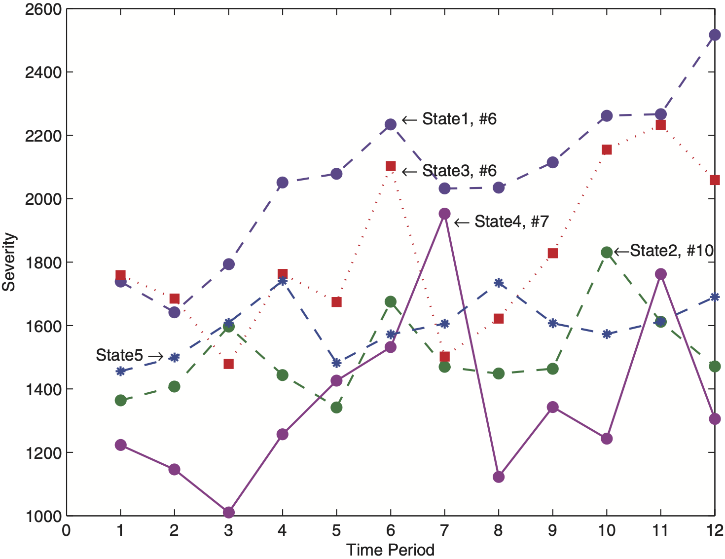
Hachemeister (1975) considered τ = 12 periods, from the third quarter of 1970 to the second quarter of 1973, of claim data for bodily injury that are covered by a private passenger auto insurance. The response variable of interest to the actuary is the severity average loss per claim, denoted by y_it. It is followed over the periods t = 1, . . . , τ_i = τ for each state i = 1, . . . , I. Average losses were reported from I = 5 different states (Appendix, Section 7.1).

A multiple time series plot of the observed variable average loss per claim, y_it, is provided in Figure 1. The plot indicates that states differ with respect to their within-state variability and severity. State 1 reports the highest average losses per claim, whereas State 4 seems to have larger variability compared to other states. For all five states we observe a small increase of severity over time. Since y_it varies over states and time (periods t = 1, . . . , 12), these characteristics are important explanatory variables. Therefore, Hachemeister originally suggested using the linear trend model given by

$$y_{i t}=\mathbf{x}_{i t} \beta+\mathbf{z}_{i t} \alpha_{i}+\varepsilon_{i t}, \tag{1}$$

where p = q = 2 in (5) and $\mathbf{x}_{i t}=\mathbf{z}_{i t}=(1, t)$. This results in a random coefficients model of the form $\mathbf{y}_i=\mathbf{X}_i\left(\beta+\alpha_i\right)+\varepsilon_i$, with diagonal matrix $\mathbf{R}_i = \mathbf{Var}\left(y_i \mid \alpha_i\right)=\operatorname{Var}\left(\varepsilon_i\right)=\sigma_{\varepsilon}^2 \operatorname{diag}\left(v_{i 1}^{-1}, \ldots, v_{i t}^{-1}\right)$, where υ_it > 0 are some known (potential) volume measures. By assumption (b) in Section 7.2, we consider independent (unobservable) risk factors that have variance-covariance structure $D=\operatorname{diag}\left(\sigma_{\alpha_1}^2, \sigma_{\alpha_2}^2\right)$. Notice that the quarterly observations #6 in State 1, #10 in State 2, #7 in State 4, and maybe #6 in State 3 seem to be apart from their state-specific inflation trends (see Figure 1).

Figure 1.Multiple time series plot of the variable average loss per claim, y_it

We use Hachemeister’s regression model (1) as our reference model to facilitate comparison of CATL credibility with other estimators discussed by the authors mentioned above. We also consider a revised version of Hachemeister’s model. When applying the linear trend model to bodily injury data, Hachemeister (1975) obtained unsatisfying model fits due to systematic underestimation of the regression line. Bühlmann and Gisler (1997) suggest taking the intercept of the regression line centered at the mean time (instead of the origin of the time axis). This ensures that the regression line stays between the individual and collective regression lines. Accordingly, we choose design matrices $\mathbf{X}_i=\left(\mathbf{x}_{i 1}, \ldots, \mathbf{x}_{i \tau}\right)^{\prime}$ and $\mathbf{Z}_i=\left(\mathbf{z}_{i 1}, \ldots, \mathbf{z}_{i \tau}\right)^{\prime}$, with $\mathbf{x}_{i t}=\mathbf{z}_{i t}=$ (1, t − G_i)′, where $G_i=v_{i .}^{-1} \Sigma_{t=1}^\tau t v_{i t}$, is the center of gravity of the time range in risk i, and $v_{i \cdot}=\sum_{t=1}^\tau v_{i t}$.

3.2. Model estimation, outlier detection, and model inference

For Hachemeister’s regression credibility model and its revised version (R), we use ln(y_it) as response variable in the framework of adaptively truncated likelihood credibility. Then, we fit (log-normal) models of the form

$$\ln \left(y_{i t}\right)=\mathbf{x}_{i t} \beta+\mathbf{z}_{i t} \alpha_{i}+\varepsilon_{i t}=\lambda_{i t}+\varepsilon_{i t}, \tag{2}$$

where $\varepsilon_{i t} \sim N\left(0, \sigma_{\varepsilon_{i t}}^2\right)$. First of all, we assume that error terms are serially uncorrelated and process variances are equal for all states, so that $\sigma_{\varepsilon_i}^2=\sigma_{\varepsilon}^2$. This yields the unweighted covariance matrix $\mathbf{R}_i=\mathbf{R}=\sigma_{\varepsilon}^2 \mathbf{I}_{\tau \times \tau}$, i = 1, . . . , I, as special case of (1). Results of the fitted model using CATL based on Henderson’s Mixed Model equation (H) are presented in Table 1. In real-data sets where the within-risk variability differs considerably from risk to risk, it is more appropriate to model unequal process variances when using CATL methods. As noted by Dornheim (2009), this assumption is rather significant for detection of atypical data points. Figure 1 indicates substantial differences in within-risk variability among the states. Hence, we fit model (2) twice, once when assuming equal (E) process variances and another time for unequal (U). Here is a summary of all the notations used in Tables 1–3:

• REML H and REML HR: REML fitting, based on Henderson’s mixed model equations, of Hachemeister’s model (REML H) and Hachemeister’s-revised model (REML HR).

• CATL HE and CATL HU: CATL fitting, based on Henderson’s mixed model equations, of Hachemeister’s model using the assumption of equal process variances (CATL HE) and unequal process variance (CATL HU).

• CATL HRE and CATL HRU: CATL fitting, based on Henderson’s mixed model equations, of Hachemeister’s revised model using the assumption of equal process variances (CATL HRE) and unequal process variance (CATL HRU).

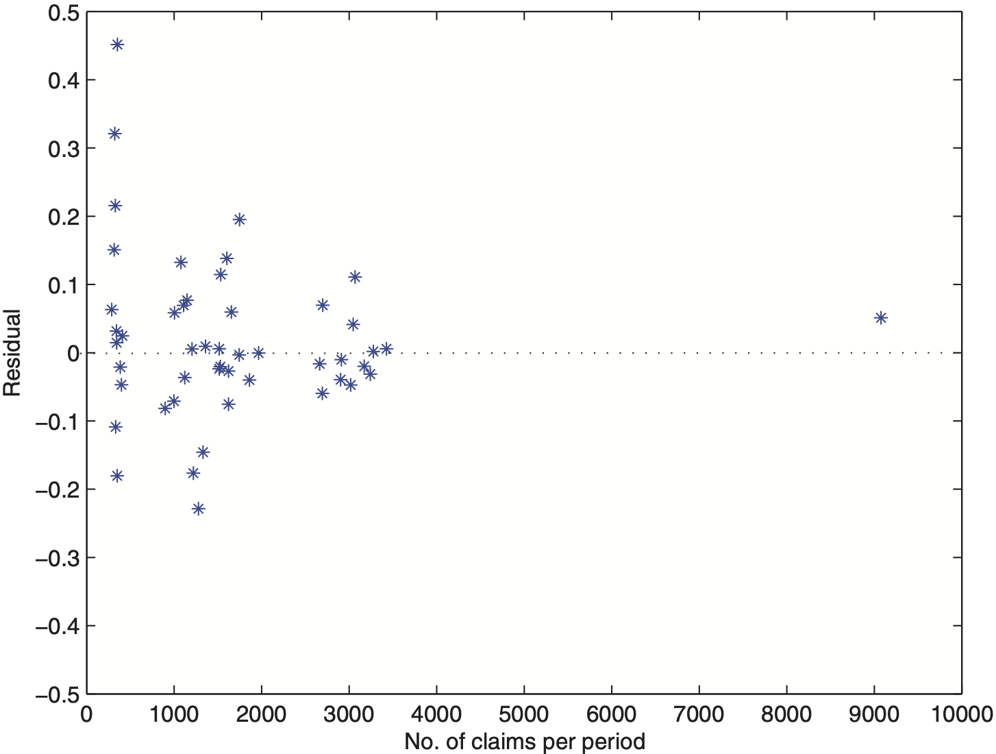
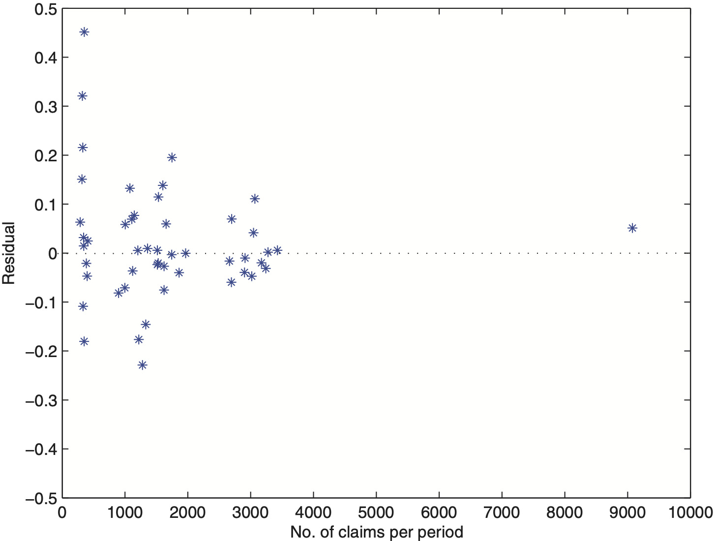
Scenario 1 denotes the real-data set used by Hachemeister. We report fixed effects β (intercept and slope) and for each state credibility adjusted estimates and predicted average claim sizes (premiums for the next period, t = 13). Further, in Figure 2 we plot residuals from the fitted log-Hachemeister model (2) versus the potential exposure measure, number of claims per period. The megaphone-shaped picture reveals that the logarithmic transformation of average loss per claim did not remove heteroscedasticity of error components. Thus, additional weighting is required. In practice, it is common to observe situations where risks with larger exposure measure typically exhibit lower variability (Kaas, Dannenburg, and Goovaerts 1997; Frees, Young, and Luo 2001). Here, it seems that number of claims per period, denoted by υ_it, significantly affects the within-risk variability. Indeed, the data set presented in the appendix supports this fact. In comparison to number of claims, State 4 reports high average losses per claim. This, in turn, yields to the increased within-state variability that is noticeable in Figure 1.

Figure 2.Scatter plot of residuals versus number of claims per period

To obtain homoscedastic error terms, we fit models using υ_it as subject-specific weights. This model can be written as

$$\ln \left(y_{i t}\right)=\mathbf{x}_{i t} \beta+\mathbf{z}_{i t} \alpha_{i}+\varepsilon_{i t} v_{i t}^{1 / 2},$$

where {ε_it} is an i.i.d. sequence of normally distributed noise terms. Similarly, the classical linear trend model as described by Hachemeister becomes

$$y_{i t}=\mathbf{x}_{i t} \beta+\mathbf{z}_{i t} \alpha_{i}+\varepsilon_{i t} v_{i t}^{1 / 2} .$$

In view of the latter regression equation, Hachemeister’s model can be considered as generalization of the weighted Bühlmann-Straub model.

Our findings for fitting of weighted regression models to Hachemeister’s data are shown in Table 2, together with the results obtained from other prominent estimation procedures. The base model is the linear trend model estimated by Goovaerts and Hoogstad (1987). To investigate the influence of the pursued procedure for estimation in Hachemeister’s regression model, Frees, Young, and Luo (1999) implemented several combinations of estimation methods (R = REML, M = Maximum likelihood), iteration methods (N = Newton-Raphson, F = Fisher-Scoring), and starting values (M = Rao’s MIVQUE(0), S = Swamy’s moment estimator) in SAS using the package PROC MIXED. Moreover, the authors distinguish between constraining the estimator of the variance-covariance matrix D, D̂, to be positive definite (Y) or not (N). In order to limit distorting effects of within-risk outliers on the assessment of individual’s claim experience, Pitselis (2002) applied MM- and GM-estimators to Hachemeister’s regression model. We denote these approaches by MM-RC and GM-RC, respectively. As an extension of his joint work about robust estimation in the Bühlmann-Straub model (Garrido and Pitselis 2000), Pitselis (2008) also employs regression M-estimators (M-RC) that are based on Hampel’s influence function approach (Hampel et al. 1986). Here is a summary of all the additional notations:

• Base: Linear trend model (Goovaerts and Hoogstad 1987).

• RNMY and RNMN: REML fitting; Newton-Raphson iteration method; Rao’s MIVQUE(0) starting values; Estimator of variance-covariance matrix is constrained to be positive definite = Yes (RNMY) and = No (RNMN). (Frees, Young, and Luo 1999).

• RFSY and RFSN: REML fitting; Fisher-Scoring iteration method; Swamy’s starting values; Estimator of variance-covariance matrix is constrained to be positive definite = Yes (RFSY) and = No (RFSN). (Frees, Young, and Luo 1999).

• MNMY and MNMN: Maximum likelihood fitting; Newton-Raphson iteration method; Rao’s MIVQUE(0) starting values; Estimator of variance-covariance matrix is constrained to be positive definite = Yes (MNMY) and = No (MNMN). (Frees, Young, and Luo 1999).

• MFSY and MFSN: Maximum likelihood fitting; Fisher-Scoring iteration method; Swamy’s starting values; Estimator of variance-covariance matrix is constrained to be positive definite = Yes (MFSY) and = No (MFSN). (Frees, Young, and Luo 1999).

• M-RC: Robust credibility based on M-estimators. (Pitselis 2008).

• MM-RC and GM-RC: Robust credibility based on multiple M-estimators (MM-RC) and generalized M-estimators (GM-RC). (Pitselis 2002).

The reliability of credibility estimates, $\hat{\mu}_{i, \tau+1}$, is of major concern to the insurer. In particular, down-biased predictions result in too-low portfolio premiums, which in turn lead to insufficient funding and threatening of the insurer’s solvency in the long run. To assess the quality of assigned credibility premiums we also report their standard errors in Table 2. These can be used to construct prediction intervals of the form BLUP (credibility estimate $\hat{\mu}_{i, \tau+1}$) plus and minus multiples of the standard error (Frees, Young, and Luo 1999). Here, we estimate the standard error of prediction, $\hat{\sigma}_{\hat{\mu}_{i, \tau+1}}$, from the data using the common nonparametric estimator

$$\begin{aligned} \hat{\sigma}_{\hat{\mu}_{i, t+1}} & =\left[\widehat{\operatorname{MSE}}\left(\hat{\mu}_{i}\right)-\widehat{\operatorname{biaS}}^{2}\left(\hat{\mu}_{i}\right)\right]^{1 / 2} \\ & =\left[v_{i \cdot}^{-1} \sum_{i=1}^{\tau} \omega_{i t} v_{i t}\left(\hat{\mu}_{i t}-y_{i t}\right)^{2}-\left(v_{i \cdot}^{-1} \sum_{i=1}^{\tau} \omega_{i t} v_{i t}\left(\hat{\mu}_{i t}-y_{i t}\right)\right)^{2}\right]^{1 / 2}, \end{aligned}$$

where µ̂_it denotes the credibility estimate obtained from the pursued regression method, υ_i⋅ is the total number of claims in state i, and ω_it is the hard-rejection weight for the observed average loss per claim y_it when employing the CATL procedure. For non-robust REML where no data points are truncated, we put ω_it = 1 as special case.

Discussion of Table 2

Let us start with Hachemeister’s linear trend model. We observe that REML estimates based on Henderson’s Mixed Model Equations, REML H, and the resulting predictions mirror findings of Frees, Young, and Luo (1999) who investigated the influence of several combinations of computation methods for classical credibility. When applying corrected adaptively truncated likelihood methods, CATL HE/U, for States 1, 3, and 5, we record credibility estimates (predictions) that are similar to those of standard approaches or robust regression techniques discussed by Pitselis (2002, 2008). For the second and fourth state, CATL HE/U determines slightly lower premiums. For instance, State 4 CATL HU yields 1447, whereas the base model by Goovaerts and Hoogstad (1987) finds 1507. This can be traced back to the removal of the suspicious observations #6 and #10 in State 2 and #7 in State 4. Robust methods employed by Pitselis (2002, 2008) hardly react to these potential outliers. This is mainly due to the subjectively chosen truncation points c and k, which may be inappropriate (too high). CATL HU also detects claim #4 in State 5 as an outlier and assigns negligible excess premiums (discounts) of −1.47 per risk. For the revised linear trend model (R) patterns are similar.

Discussion of Figure 3

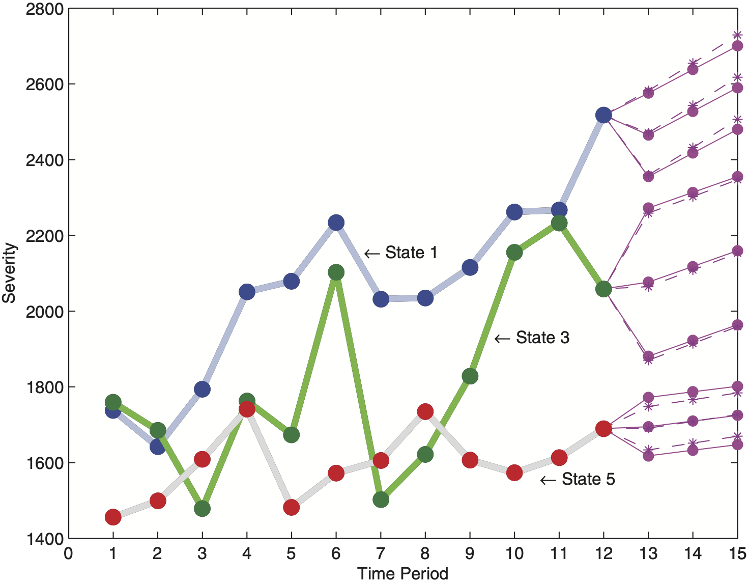
We display in Figure 3 the three-step predictions of the average loss per claim for States 1, 3, and 5 when using REML H and CATL HU. The thinner lines show predictions and one standard error of the prediction for each of the three states. These can be compared to Frees, Young, and Luo (1999, Figure 1). Note, the less variable States 1 and 5 have shorter prediction intervals compared to State 3. As expected, in Scenario 1 predictions and intervals obtained from REML and CATL HU nearly coincide.

Figure 3.Selected severity predictions based on Hachemeister’s model (weighted) and data. The thinner middle line marked by ● denotes one-, two-, and three-step predictions using REML H. The upper and lower lines complete the one standard error prediction interval. Predictions from the CATL HU procedure are marked by *

To illustrate robustness of regression credibility methods that are based on M-RC, MM-RC, and GM-RC estimators for quantifying individual’s risk experience, Pitselis (2002, 2008) replaces the last observation of the fifth state 1690 by 5000 (Scenario 2). We follow the same contamination strategy and summarize outcomes in Table 3. It turns out that the choice of the methodology has a major impact on the fitting of credibility models.

Discussion of Table 3

In the presence of a single outlier in Scenario 2, it is not surprising that standard statistical methods react dramatically. In the contaminated State 5, the REML H and base credibility estimate of Goovaerts and Hoogstad (1987) get highly attracted by the outlying observation and increase from 1695 to 2542 and from 1759 to 2596, respectively. Further, it is well known that the occurrence of outliers distorts the estimation process of variance components and, hence, yields too-low credibility weights. As a consequence, credibility adjusted estimates are pulled toward the increased grand mean (most notably the slope component) which results in inflated credibility premiums and prediction intervals across all states. In particular, for REML H the estimated standard error in State 5 explodes from 77 to 829 due to enhanced within-risk variability that is caused by the single catastrophic event. Even though only the fifth contract is contaminated, the portfolio-unbiased regression M- and GM-credibility estimators with chosen tuning parameters c = 1.345 and k = 2, respectively, are significantly distorted. Indeed, these estimators provide protection in the assessment of the individual state experience. However, they reveal a substantial lack of robustness toward single large claims that have adverse effects on the between-risk variability as well. Consequently, the entire estimation process for states that have merely small claims (e.g., see State 2) also becomes distorted. These deficiencies have been removed by CATL estimators. We observe that CATL HU still provides reasonable credibility premiums for all contracts in the portfolio. Both the grand location, λ̂ = (7.28, 0.016), the credibility adjusted estimates, λ̂_i, the estimated standard errors, and predictions of expected claims remain stable. We shall emphasize that the latter changes only marginally from 1691 to 1689 in the contaminated State 5. The CATL HU identifies the single large claim and distributes uniformly an extraordinary premium of 4.33 to all contracts.

In Figure 4 we visualize the impact of a single outlier on the premium ratemaking process. When using classical regression techniques such as REML, the contaminated contract elevates the grand mean of all states, most of all the forecasted credibility premium and its prediction interval in State 5. Clearly, CATL provides robustness for adequate inference in Hachemeister’s regression model.

Figure 4.Selected severity predictions based on Hachemeister’s model (weighted) and data. The thinner middle line marked by ○ denotes one-, two-, and three-step predictions using REML H. The upper and lower lines complete the one standard error prediction interval. Predictions from CATL HU are marked by *

4. Medicare data

In this section, we apply CATL procedures to a health care data set that contains Medicare costs for inpatient hospital charges. This real-data set has been examined by Frees, Young, and Luo (2001) to demonstrate that general mixed linear models can be used to produce credibility estimates of future claims.

4.1. Data characteristics

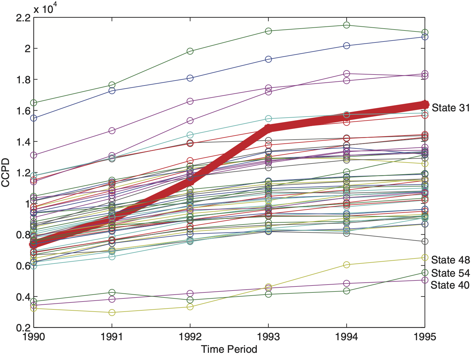
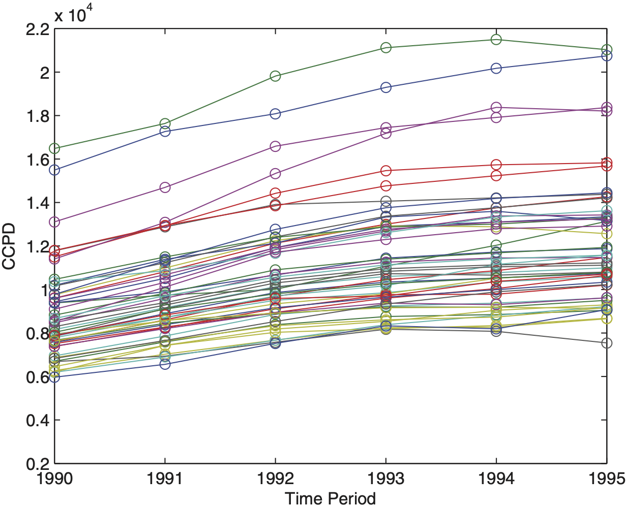
The underlying health care data set for Figure 5 has been published by the Health Care Financing Administration and reports inpatient hospital charges over τ = 6 years, from 1990 to 1995. These charges have been covered by the Medicare program in I = 54 states across the United States, including the District of Columbia, Virgin Islands, Puerto Rico, and an unspecified category, in addition to the 50 states.

Figure 5.Multiple time series plot of covered claims per discharge (denoted by CCPD) over the years 1990 to 1995

The Medicare program reimburses hospital claims on per-stay basis, hence, the dependent variable is covered claims per discharge, denoted by CCPD. The multiple time series plot in Figure 5 indicates that there is rather substantial variability among the states and some variability over the time. Therefore, it is natural to explain the response at least by the regressors state and time. Frees, Young, and Luo (2001) investigated several possible explanatory variables through graphical tools and found that the component average hospital stay per discharge in days, denoted by AVE_DAYS, is a statistically significant predictor.

More interestingly, the state of New Jersey (State 31) reveals a notably greater increase of CCPD over the years 1990 to 1993. Frees, Young, and Luo (2001) identify this outlying growth of medical costs and take it explicitly into account in their model by incorporating a state-specific correction term for the time slope in New Jersey. Further analysis (e.g., employing scatter plots) shows that the second observation of the 54th state is explained by an unusually high hospital utilization AVE_DAYS. Thus, this data point that has large distorting effects on classical estimation procedures, such as REML, has been manually removed by the authors (see Frees, Young, and Luo 2001, Table 1, Figure 4). In Figure 5 we observe that two other outlying risks are State 40 and 48. These states report relatively low CCPD over time and, thus, have a distorting effect on the estimation of between-state variability.

4.2. Model fitting, outlier detection, prediction

For CATL we fit an error components model of the form

$$\begin{aligned} \ln \left(C C P D_{i t}\right)= & \beta_{1}+\beta_{2} Y E A R_{t}+\beta_{3} A V E_{-} D A Y S_{i t} \\ & +\alpha_{i 1}+\alpha_{i 2} Y E A R_{t}+\varepsilon_{i t}, \end{aligned} \tag{3}$$

where β = (β₁, β₂, β₃)′ is the grand location, α_i = (α_i1, α_i2)′ are the unobservable random effects, and $\mathbf{x}_{i t}=\left(1, t, A V E_{-} D A Y S_{i t}\right)$ and $\mathbf{z}_{i t}=(1, t)$ are the corresponding explanatory variables for i = 1, . . . , I = 54 states followed over the periods t = 1, . . . , τ = 6. Frees, Young, and Luo (2001) found that no weighting by some exposure measure is required to accommodate potential heteroscedasticity in the data. Therefore, we model the serially uncorrelated error terms by the unweighted variance-covariance matrix $\mathbf{R}_i=\sigma_{\varepsilon}^2 \mathbf{I}_{\tau \times \tau}$, where ε_it ∼ N(0, σ²_ε) for all states. This model can be viewed as an extension of Hachemeister’s linear trend model in Section 3. It is similar to the preferred mixed linear model in Frees, Young, and Luo (2001), denoted by Model 6. Note, however, that their model includes an additional special interaction variable to represent the atypical large time slope in State 31 and is given by

$$\begin{aligned} C C P D_{i t}= & \beta_{1}+\text { YEAR }_{t}\left(\beta_{2}+\beta_{4} 1\{\text { State }=31\}\right) \\ & +\beta_{3} \text { AVE_DAYS } S_{i t}+\alpha_{i 1}+\alpha_{i 2} \text { YEAR }_{t}+\varepsilon_{i t}, \end{aligned} \tag{4}$$

where β₂ + β₄1 {State = 31} + α_i2 can be interpreted as the New Jersey–specific total contribution of the regressor YEAR.

In our analysis, the CATL procedure detects and rejects all suspicious data points that have been identified by laborious graphical tools in Frees, Young, and Luo (2001) and, therefore, supersedes the modeling of New Jersey–specific covariates. Results of the detection process using CATL with equal process variances are visualized in Figure 6. We see that State 31 (New Jersey) has an extraordinary high time slope, States 40, 48 and 54 have unusual low intercepts, and the second observation of the 54th state (though not visible in Figure 6) has been entirely removed.

Figure 6.Multiple time series plot of covered claims per discharge (denoted CCPD) over the years 1990 to 1995 after data cleaning

In Table 4 we provide results of fitted regression models based on Equation (4) for Model 6 in Frees, Young, and Luo (2001), and on Equation (3) for the CATL approaches 1 and 2. Here, approach 1 denotes the Medicare data set containing all 54 states, whereas the outlying States 31 and 54 have been deleted for approach 2. Note that our REML estimates do not incorporate the New Jersey–specific time slope.

Discussion of Table 4

When the entire data set is considered (approach 1) we observe that the standard method REML 1 gets attracted by the outlying data points and produces estimates of fixed effects that differ significantly from those of Model 6. For instance, β₃ is 348.3 for Model 6 versus 21.9 for REML 1. Also, REML 1 finds the time slope β₂ = 675.3 for all states. However, the mean slope of the state of New Jersey should be much steeper (β₂ + β₄ = 753.1 + 1540.81) as indicated by Model 6 and Figure 7. Once the States 31 and 54 have been eliminated (REML 2), these standard estimates are comparable to those in Model 6 but still do not account for the extraordinary increase of hospital costs in State 31. As expected, the robust CATL procedure provides protection against catastrophic events, and we do not observe any significant differences between the estimates obtained when employing CATL 1 or CATL 2. Also, Figure 7 shows that the robust procedures allow for the greater rate of inflation of Medicare costs in New Jersey.

Figure 7.The years 1990–1995 represent actual CCPD for selected states New Jersey (State 31), Virgin Islands (State 48), and “Other” (State 54). For 1996–1998, the middle line, marked by ○, denotes the one-, two-, and three-step predictions using REML. The upper and lower lines complete the two standard deviations interval. Predictions and intervals obtained from CATL are marked by ●

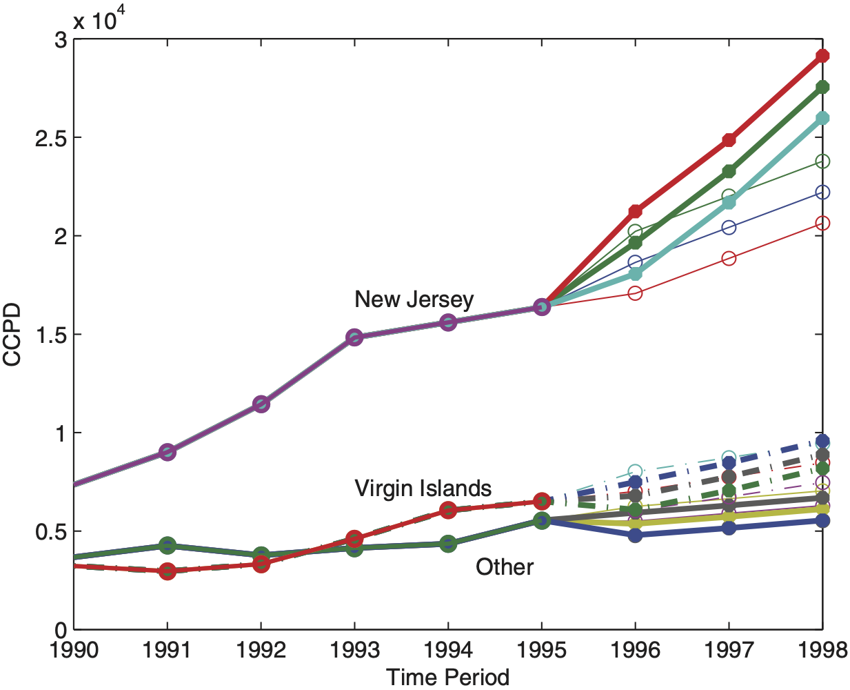
For the computation of one-, two-, and three-step predictions over the years 1996–1998, we assume that the most recent subject-specific average hospital utilizations per discharge (AVE_DAYS$\mathstrut_{it}$) remain constant, i.e., AVE_DAYS$\mathstrut_{i6}$ = AVE_DAYS$\mathstrut_{i7}$. Then, in Table 5 we give the grand mean β̂ and selected credibility adjusted estimates β̂_i when using REML 1. Likewise, the grand location and credibility-adjusted locations are summarized for CATL 1. The resulting credibility estimates for the expected CCPD_it as well as the estimated standard errors for construction of prediction intervals, are registered over the forecasted periods t = 7, 8, 9, that represent the years 1996 to 1998.

Discussion of Figure 7

Most of the findings that are outlined in Table 5 for the selected states New Jersey, Virgin Islands, and “Other” can be visualized in Figure 7. We see that credibility estimates for Virgin Islands and “Other” are similar. However, we observe that the prediction intervals obtained from CATL are somewhat shorter. For instance, this is due to the removal of the second data point in the 54th state. Let us focus on predictions in the state of New Jersey. As indicated by results recorded in Table 4, it becomes apparent that REML significantly underestimates the inflation trend of Medicare costs. In contrast, CATL produces suitable forecasts for CCPDs. We shall also emphasize that intervals based on CATL are shorter.

5. Housing prices in U.S. metropolitan areas

In the case study of this section, we analyze annual housing prices in U.S. metropolitan statistical areas (MSAs). In view of the previous two sections, where Section 3 falls directly in traditional property/casualty field and Section 4 follows the health insurance practice, this type of data is not what actuaries concentrate on currently in their work. With this choice of data we clearly venture outside the actuary’s comfort zone, but hope to provide additional insights, highlight the versatility of these advanced techniques, and broaden their area of application.

In this section, we employ graphical tools and statistical criteria to

• view data,

• find atypical data points, and

• evaluate the reliability of the newly designed robust approach as diagnostic tool.

We also compare fitted parameters of robust CATL with classical REML. The data set we consider is taken from Frees (2004) and had been studied originally by Green and Malpezzi (2003).

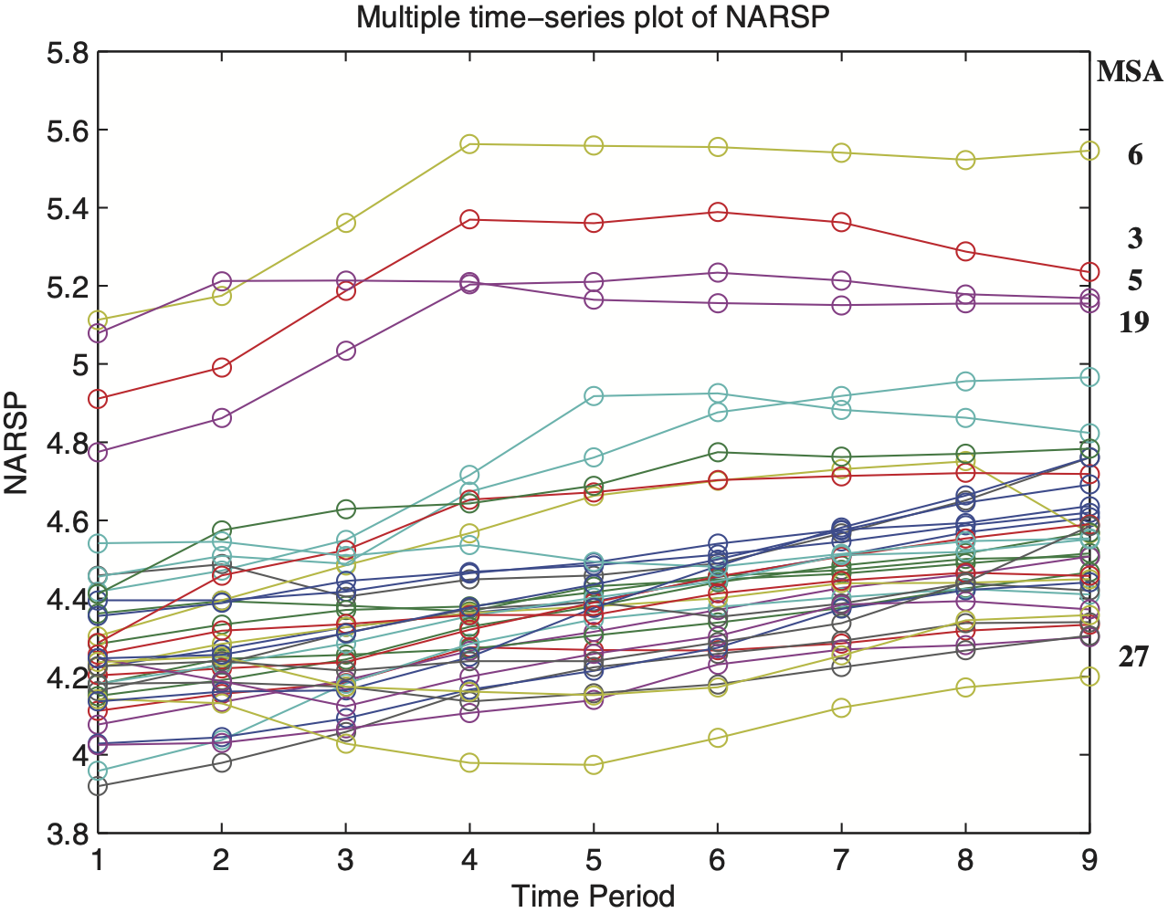
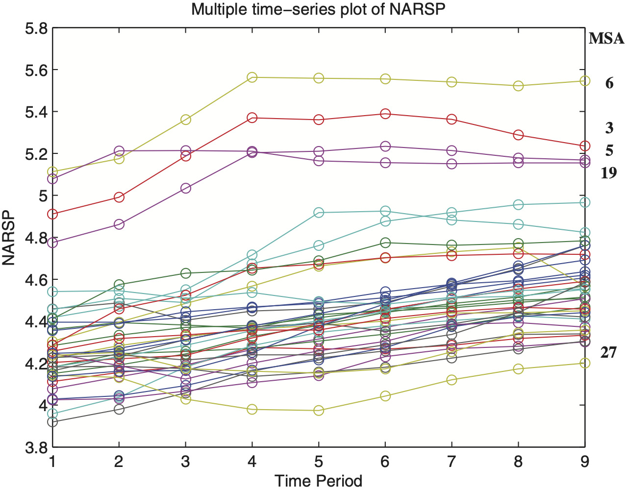
We investigate the influence of the demand-side variables annual percentage growth of per capita income (PERYPC) and annual percentage growth of population (PERPOP) on the response NARSP. The response variable NARSP represents the MSA’s average sale price in logarithmic units and is based on transactions reported through the Multiple Listing Service, National Association of Realtors. The balanced data set contains I = 36 MSAs with n = 9 annual observations each, over the years 1986 to 1994. We fit an error components model of the form

$$\begin{aligned} \text { NARSP }_{i t}= & \mu+\beta_{1} \text { PERYPC }_{i t}+\beta_{2} \text { PERPOP }_{i t} \\ & +\beta_{3} \text { YEAR }_{i}+\alpha_{i}+\varepsilon_{i t}, \end{aligned}$$

where i = 1, . . . , I, t = 1, . . . , n_i = n, µ is the population grand mean, α_i is the metropolitan-specific random intercept, and β = (β₁, β₂, β₃)′ is the fixed effects of time-dependent explanatory variables PERYPC_it, PERPOP_it, and YEAR_t, respectively. We assume that the error terms are serially uncorrelated, so that $\mathbf{R}_i=\sigma_{\varepsilon_i}^2 \mathbf{I}_{n \times n}$.

5.1. Data characteristics

In this subsection, we characterize the housing sales price data using graphical and common statistical tools. Table 6 summarizes the response variable NARSP by MSA. We see that MSAs vary in their average and median NARSPs. In particular, average sales prices recorded for metropolitan areas #3, #5, #6, and #19 both start and close at comparatively high price levels. We also observe that the within-MSA variability (Std. Dev.) indicates substantial differences among MSAs. For instance, we record an extremely high variability of 0.24 for MSA #29 versus nearly negligible variations of as low as 0.03 for MSA #32. These MSAs are considered to be outlying with respect to their unusually high/low within-MSA variability. These patterns are highlighted when considering the total variation of yearly percentage-change in NARSP. (Note that the total variation of yearly percentage-change in NARSP is computed as the sum of the eight absolute percentage-changes for each NARSP observed over a 9-year period.)

Table 7 provides summary statistics for NARSP by year. We observe that almost all statistical quantities increase over time except for the overall variation (Std. Dev.) in the data. These do not hint at any significant time-dependency.

Figure 8 is a multiple time series plot of NARSP and provides a visualization of the findings in Tables 6 and 7. We see that not only are overall NARSP increasing in time but also that average house sale prices increase for each MSA. Indeed, as Figure 8 indicates, there is substantial variability among MSAs, not just a simple time trend. This plot also reveals that MSAs #3, #5, #6, #19, and #27 stay permanently away from the majority of data, which is seen from unusually high (low) subject-specific intercepts. Finally, this preliminary analysis will help us to understand how few atypical MSAs can have disturbing effects on classical estimation of variance components. It turns out that the robust CATL procedure can provide major improvements in model fit over the non-robust REML.

Figure 8.Multiple time series plot of NARSP over n = 9 years, 1986–1994. The line segments connect metropolitan statistical areas (MSAs).

5.2. Model fitting and outlier detection

We find CATL estimates under the following assumptions for residuals: identically distributed, i.e., $\varepsilon_{i t} \sim N\left(0, \sigma_{\varepsilon}^2\right)$, and non-identically distributed, i.e., $\varepsilon_{i t} \sim N\left(0, \sigma_{\varepsilon_i}^2\right)$. As discussed in a previous section, this assumption is rather significant for detection of atypical data points. In the current example, the assumption of equal error variances allows us to identify such MSAs as outlying when their individual within-subject variation is comparatively high or low. By contrast, when assuming unequal error variances, the CATL procedures only detect those MSAs for which random effects appear to be extreme.

Discussion of Table 8

CATL estimates for the grand mean µ̂ are lower than those from REML, which was expected. This effect can be traced back to the identification and elimination of extreme MSAs having rather high NARSP over time (Table 6). As a result, we record substantially reduced estimates for variance components σ²_α and σ²_ε. In particular, when removing MSAs #3, #4, #5, #6, #11, #19, #27, #28, #29, and #32 from the data, the between-MSA variability σ̂²_α drops dramatically from 0.097 (REML) to as low as 0.018 (CATL, identical). This is accompanied by a reduction of the overall within-subject variability σ̂²_ε from 0.005 (REML) to 0.003 (CATL, identical). That is, when assuming identically distributed error terms, the CATL methods eliminate MSAs where either individual random intercepts are extreme or their within-subject variability differs clearly from the most typical one. Note that the CATL procedure reliably removes all extraordinary MSAs that have been detected using laborious and time-consuming graphical tools. For CATL methods with non-identical error variances the latter type of extremes is ignored, hence fewer MSAs are truncated from the data, and thus, the estimated variance component σ̂²_α is slightly increased to 0.026. Now, only the MSAs #3, #5, #6, and #19 that have atypical high intercept are marked as extraordinary. We see that the estimates for fixed effects are of the same magnitude.

6. Summary

In this paper, we have illustrated how corrected adaptively truncated likelihood methods, CATL, can be used for robust-efficient fitting of general regression-type models with heavy-tailed data. We have seen that this procedure is a flexible and effective risk-pricing tool. This has been demonstrated through three well-studied examples from the fields of property and casualty insurance, health care, and real estate. In particular, we have shown the entire process of data analysis, model selection, outlier identification, and the associated statistical inference.

Further, a number of observations can be made based on our analysis. In particular, for Hachemeister’s bodily injury data, we notice that CATL methods (a) allow to mitigate heteroscedasticity through explicit incorporation of weighting and/or use of logarithmic transformation; (b) accommodate within-risk variability through modeling of subject-specific process variance; (c) provide high robustness against outliers occurring both within and between risks through adaptive detection rules that automatically identify and reject excess claims in samples of small size; (d) provide robust credibility premiums; (e) demonstrate efficiency and reliability of detection rules, therefore making the use of graphical tools (for identification of outliers) and expert judgment (for the choice of truncation points) non-essential; and (f) compete well against established robust methods. Analysis of the Medicare and the house-pricing data sets just reinforces our findings.

Furthermore, for the readers who are interested in implementing CATL methods, the matlab computer code is available from the authors upon request. Also, we shall emphasize again that one should be careful about the automatic nature of “data cleaning” and model fitting exhibited by CATL methods (see comments c and e above). This aspect of the methodology is an important improvement, as it makes the process of statistical modeling easier and quicker. However, it does not imply that the actuary may now ignore such crucial issues as understanding of the practical problem, its context, available data, and the economic consequences of the model-based decisions.

Finally, the case studies in this paper were focused and did illustrate various statistical aspects of the CATL approach. What is equally important and interesting is to compare this methodology with some well-established and actuarially sound techniques. For instance, one method that is often used in practice is to set the overall portfolio rate level and then use predictive modeling techniques to allocate the rates between classes. This will be a topic for future research project.

Acknowledgments

The authors gratefully acknowledge the support provided by a grant from the Casualty Actuarial Society. We also are very appreciative of useful comments, suggestions, and valuable insights provided by two anonymous referees that helped to significantly improve the paper.