A Data-Based Assessment of the Impact of Marijuana Legalization on Vehicle Accident Experience

1. Introduction

Private cars are essential for many people living in the U.S. and Canada and have been an attribute of material prosperity. The insurance risks related to cars have been affected in recent years by regional changes in the legal rules on using marijuana. Legalization of marijuana in several regions was associated with a higher number of drivers operating vehicles under the influence of the drug (Pollini et al. 2015) and more car crash fatalities (Cook, Leung, and Smith 2020). While the debates and decisions in the process of legalization of marijuana continue, insurance companies need to assess the associated changes in vehicle accident experience to price the risk and adjust the cost of insurance.

There have been mixed reports about the implications of legalization of marijuana (e.g., see a brief overview by Hall and Lynskey [2020]), which could be explained in part by the fact that the studies consider only one region (data limitation) or rely on only one statistical method. Other publications consider relative change without the overall impact; for example, Pollini et al. (2015) studied the proportion of drivers who tested positive for delta-9-tetrahydrocannabinol (THC), not the changes in the number or severity of car accidents.

This study proposes data-driven tools for assessing the impact of changes in marijuana laws on vehicle accident experience by harnessing the publicly available data with the power of modern statistical and machine learning techniques under the integrative framework for impact analysis and uncertainty quantification.

1.1. Approach

The study provides new insight into the impacts of marijuana legalization on the vehicle accident experience and the implications for the insurance industry and develops a systematic approach for assessing similar types of changes in the future. To establish a robust causal framework that would equip the insurance industry with actionable insights for risk mitigation and pricing strategies, this study seeks to achieve the following key objectives.

1. Isolate the causal effect of legalization:

   • Establish robust control groups using either before–after analysis within regions or concurrent comparisons with similar regions.

   • Account for trends and regional variations to isolate the true effect of legalization on accident rates.

2. Mitigate the influence of confounding variables:

   • Collect and integrate data on confounding factors such as weather, time of day, and day of the week.

   • Ensure that the analysis accurately reflects the causal impact of legalization rather than external influences.

3. Harness the power of modern causal inference techniques:

   • Leverage regularization techniques to prevent overfitting and improve generalizability of findings.

   • Employ methods that calibrate p-values and confidence intervals for more reliable assessments of statistical significance.

   • Implement flexible nonparametric methods such as random forests to capture complex, nonlinear relationships.

4. Synthesize results for broad applicability:

   • Analyze data across diverse methods and geographic regions.

   • Synthesize the results to strengthen the validity and generalizability of conclusions.

The significance of this study extends beyond the case of marijuana legalization. This framework serves as a blueprint for assessing the impact of future policy changes, such as the legalization of other substances or the introduction of self-driving cars.

1.2. Literature overview of marijuana and legalization impacts

Several studies investigated (1) the impacts of marijuana on the ability to drive (controlled and observational studies); (2) the impact of legalization on the proportion of drivers who tested positive for marijuana use (observational studies); and (3) the impact of legalization on public health and safety outcomes (observational studies).

While the first two groups of studies lay down important groundwork for investigating marijuana impacts, this research and the third group of studies primarily focus on estimating aggregated effects on crashes and fatalities. The studies in this group report mixed results, most often not detecting the effects of marijuana legalization on road crashes (Hall and Lynskey 2020; Hansen, Miller, and Weber 2020). Cook, Leung, and Smith (2020) studied semiannual 2010–2017 Fatality Analysis Reporting System (FARS) data from cities with a population greater than 100,000 located in states that did not enact medical marijuana laws by 2010. Using the difference-in-differences approach, this study identified a slight reduction (9%) in fatal crashes after the adoption of medical marijuana use in the states, but no effect of legalization was detected except for young male drivers (13% increase in fatal crashes). Lane and Hall (2019) used interrupted monthly time-series analysis (2009–2016) and detected a short-term increase in FARS-reported fatalities in Colorado, Washington, Oregon, and their neighboring jurisdictions (an increase of one fatality per million residents in the year following marijuana legalization). Santaella-Tenorio, Mauro, Wall, et al. (2017) used multilevel regression models and detected some short-term reductions in fatalities associated with the legalization of medical marijuana between 1985 and 2014. Farmer, Monfort, and Woods (2022) studied quarterly crash rates per mile of travel in 11 states during 2009 to 2019, while accounting for time effects, seat belt use rate, unemployment, and alcohol use rates. The authors concluded that estimates of marijuana legalization effects are not always statistically significant and vary by state. Windle and colleagues (Windle, Eisenberg, Reynier, et al. 2021; Windle, Sequeira, Filion, et al. 2021) extend to Canada the insights drawn from the US FARS database about the effects of legalization on fatal collision rates and fatalities. Windle, Eisenberg, Reynier, et al. (2021) find evidence of increased fatal collision rates when the model adjusted for linear time trend is used; however, a comment on the paper posted online by Jiang et al. reports the Poisson model as a poor fit. Finally, Compton (2017) provides a great overview of the related research and existing practical questions related to drug testing processes, devices used, and training of personnel.

This study brings together the technical advancements of machine learning algorithms for finding patterns in data, rigorous approaches for selecting control units from observational data, and recently developed pathways for a causal interpretation of black-box models. A combination of all these steps has not previously appeared in a single study on the effects of marijuana legalization. Specifically, this study attempts to overcome the disadvantages of earlier analyses that relied on the assumed linearity (suggesting the use of nonlinear models such as random forests, where appropriate) and parametric inference (suggesting the use of bootstrapping to derive confidence intervals without relying on a particular distribution).

2. Data

For a maximally cohesive presentation for Canada and the U.S., the same study period (2016–2019) is used for both countries. To avoid confounding with the impacts of the COVID-19 pandemic, data from 2020 or later are not used. More specifically, there are no provinces in Canada that can act as a control group for estimating the effect of marijuana legalization (see Section 2.1), so the effect of the COVID-19 pandemic would be confounded with other effects. In the U.S., states serve as the controls for estimating the legalization effects (see Section 2.2), and some researchers argue that one does not need to explicitly adjust for confounders when a control group is used (Elvik 2002). However, the impacts of COVID-19, such as the mobility changes due to imposed lockdowns of different stringency, have varied considerably within states (Barnes et al. 2020), across states (Lin, Shi, and Li 2021), and globally (Gupta, Pawar, and Velaga 2021; Rahman et al. 2021; Yasin, Grivna, and Abu-Zidan 2021). Moreover, the recovery of human mobility after the relaxation of the lockdowns also differed across regions. Such trends pose additional difficulties if included in the study (e.g., see Choi et al. 2018) since confounding factors may affect sites differently in time (Smith, Orvos, and Cairns 1993).

2.1. Canada

The legalization of recreational use of marijuana took effect across Canada on October 17, 2018 (Senate of Canada 2018).^[1]

The data used in this study came from annual reports of the General Insurance Statistical Agency (2021), which collects insurance information from most Canadian regions (except British Columbia, Manitoba, Québec, and Saskatchewan), and Groupement des Assureurs Automobiles (n.d.) which provides the information for Québec. From these reports, information on the collision of private vehicles per accident year was extracted. The claims in this category are characterized by loss development factors close to 1; hence, they are not expected to change substantially as the losses from accidents that happened in the most recent years get finalized. Dollar amounts were adjusted to the prices of 2019 to account for the changing value of money, using the Consumer Price Index (all item groups) by Statistics Canada (2021).

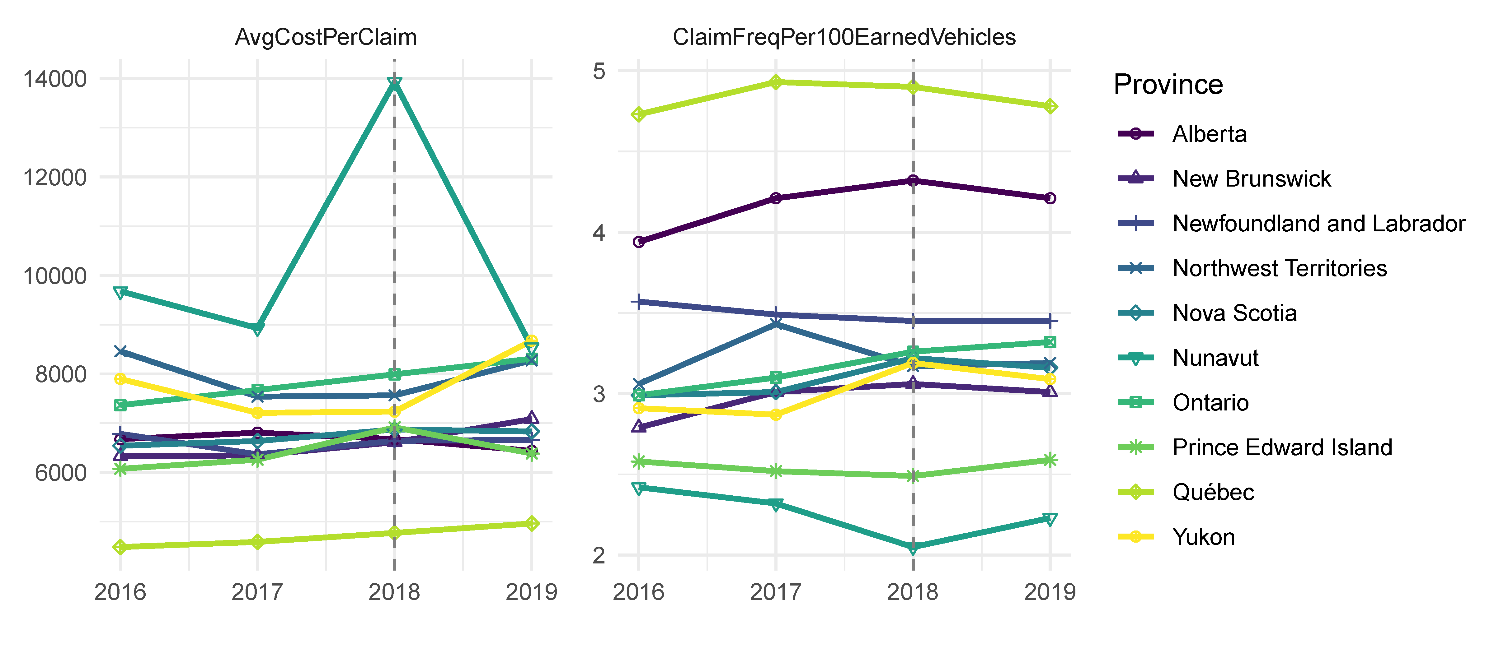
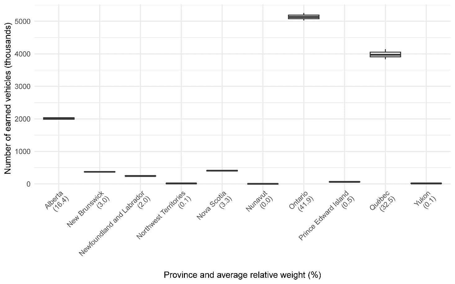
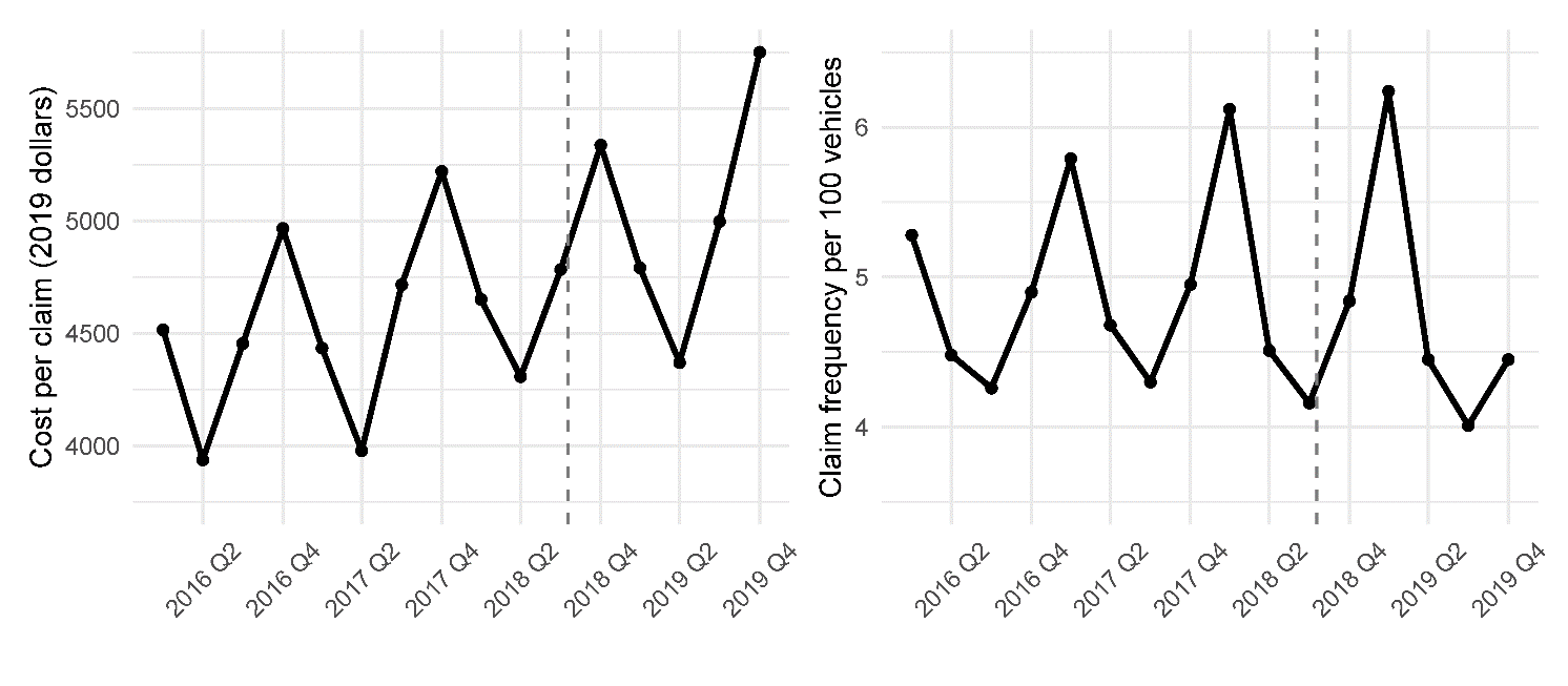
The studied insurance outcomes vary considerably across regions, more than across years (Figure 1). An extremely high average cost per claim was reported in Nunavut in 2018, but this year was also the year of the law enactment; thus, all observations from 2018 were omitted due to the difficulty of separating the annualized values into the periods before and after the legalization. The regions differ in population, so the annual number of earned vehicles was used to weight the observations in further analyses (Figure 2).

Figure 1.Annual average cost per claim (in 2019 dollars) and frequency of collisions. The dashed line denotes the year of marijuana legalization.

Figure 2.Number of earned vehicles during 2016–2019 used as the regional weights. The lower and upper hinges correspond to the first and third quartiles.

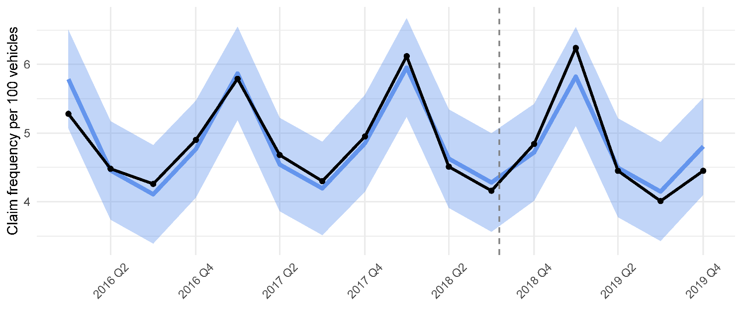
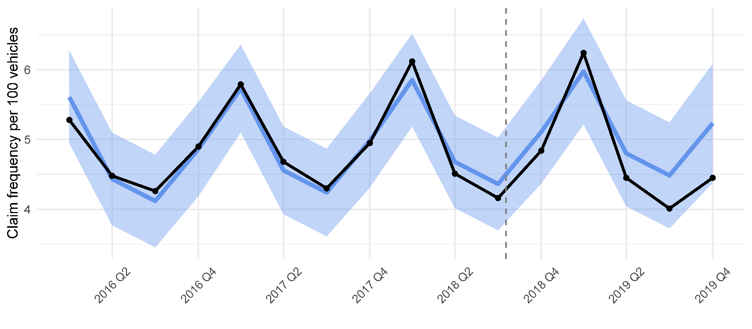
The insurance data for Québec were provided at the quarterly frequency, which allowed us to study seasonal signals (see Appendix).

2.2. United States

In the U.S., the legality of marijuana varies by jurisdiction (see Table 1 for a summary of the legalization history by state in the study period). The start of the period (early 2016) was defined by data availability in the Countrywide Traffic Accident Dataset version 4 (Moosavi et al. 2019), which was originally used in this study but later removed. Since some states (including Colorado and Washington) had already legalized marijuana by 2016, they cannot be used for the before–after comparisons in this study (see, e.g., Aydelotte, Brown, Luftman, et al. 2017 and Hansen, Miller, and Weber 2020 for the analysis of Colorado and Washington). The end of the period (December 2019, same as for Canada) was chosen to avoid confounding the estimated effects with the impacts of the COVID-19 pandemic. State-licensed sales of recreational cannabis in Michigan began on December 1, 2019 (one month before the end of the study period). For all the Before and After periods to be at least one year long for more reliable conclusions, Michigan was removed from consideration.

The following state statistics were used to select the control group states matching the legalized group: urbanization (percentage of the total population; Wikimedia Foundation 2021c), population (Office of Highway Policy Information 2021), vehicle miles per licensed driver, road miles per 1000 persons (calculated as the total road and street mileage divided by the population), and vehicles per 1000 people (Wikimedia Foundation 2021b). Number of licensed drivers was also considered but correlated too strongly (r = 0.99) with population.

The National Highway Traffic Safety Administration’s FARS (2021) was used to extract data on fatal traffic accidents, including the number of fatalities and number of fatal accidents. The database was supplemented with such variables as Year (numeric), Month (1–12, categorical), Weekday (1–7, categorical), Weekend (0/1, categorical), and Holiday (0/1, categorical, based on holiday calendar for the New York Stock Exchange, Wuertz, Setz, and Chalabi 2022). The accident experience metrics were normalized by the number of registered vehicles by year and state, available from the U.S. Federal Highway Administration (U.S. Department of Transportation 2020). The Daymet dataset (Thornton et al. 2020) was used to extract daily gridded data on confounding weather conditions, represented by precipitation amounts and temperature ranges; average temperature was computed as the mean and temperature range was computed as the difference between maximal and minimal temperatures. Numerical summaries of the variables are shown in Table A1.

3. Methods

Use two-tailed tests with significance level α = 0.05 unless noted otherwise (1 − α = 0.95 or 95% corresponds to the confidence level). In other words, the results are statistically significant when the corresponding p-values are below α. The results of the analysis can be reproduced using the R code available from Lyubchich (2024).

3.1. Before–after comparison

For simple before–after comparisons when no concurrent control is available (i.e., for Canada), the following regression models with parametric inference and residual (semiparametric) bootstrap are applied.

3.1.1. Parametric models

Consider a mixed-effects model (Zuur et al. 2009)

$$y_{tp} = a + bX_{t} + ct + \beta_{p} + e_{tp}, \tag{3.1}$$

where y is the response variable (claim frequency or average cost per claim), t is the numeric time index (year), p is the space index (province), a is the grand intercept, b and c are the fixed-effect coefficients, X is the indicator whether t is before the marijuana legalization date or after (since the law was enacted in October 2018, the year of 2018 was excluded), β_p ∼ N (0, δ²) are random intercepts accounting for different average levels of the response variable by province, and e_tp are the model residuals. Weights w_tp are applied to the residual variances for weighted estimation, such as e_tp ∼ N (0, σ²w_tp). In particular, $w_{tp} = {(Number\ of\ earned\ vehicles)}_{tp}^{- 1}$ was used to assign bigger weights to observations corresponding to more earned vehicles. The variance structure in the model also allows it to address the issue of heterogeneity or variance clustering (Abadie et al. 2023). From three alternative structures—fixed, constant by province, and power—the latter was selected based on the smallest value of the Akaike information criterion (AIC; see Zuur et al. 2009, Section 4).

The time trend was included in the model to avoid spurious regression results (e.g., see Wooldridge 2013, Section 10.5). This is possible due to the conditional interpretation of coefficients in multiple regression that might differ from marginal relationships (e.g., see Chatterjee and Simonoff 2013, Section 1.3.1). For example, the coefficient b in model (3.1) can be interpreted as the expected change in the claim frequency with marijuana legalization, holding everything else in the model fixed. In this analysis, the linear trend is appropriate for capturing the trending behavior of time series (based on the patterns in Figure 1) and hence is a preferred option for regression analysis of nonstationary series, compared with using the regression model with detrended differenced series (e.g., ∆y_t,p = y_t,p − y_t−1,p) or deviations from an estimated trend ${\widetilde{y}}_{tp}$ (i.e., ${\widehat{\epsilon}}_{tp} = y_{tp} - {\widetilde{y}}_{tp}$).

3.1.2. Bootstrap

To make the inference based on the mixed-effects models robust to non-normality, implement the semiparametric residual bootstrap algorithm (Carpenter, Goldstein, and Rasbash 2003; Loy, Steele, and Korobova 2022):

1. Estimate parameters and error terms for the model.

2. Sample independently with replacement from the sets of error terms.

3. Rescale the bootstrapped error terms so that their empirical variance is equal to the model estimates.

4. Obtain bootstrap samples by combining the bootstrapped samples via the fitted model equation.

5. Refit the model and extract the statistics of interest.

6. Repeat steps 2–5 B times.

From the bootstrapped distributions, obtain confidence intervals for the desired confidence level 1 − α, as defined in Davison and Hinkley (1997, Chapter 5). For the estimate $\widehat{b}$ and its bootstrap counterparts ${\widehat{b}}^{*}$, the basic bootstrap confidence limits are

$$2\widehat{b} - {\widehat{b}}_{\lbrack(B + 1)(1 - \alpha/2)\rbrack}^{*},\ 2\widehat{b} - {\widehat{b}}_{\lbrack(B + 1)\alpha/2\rbrack}^{*}, \tag{3.2}$$

the percentile limits are

$${\widehat{b}}_{\lbrack(B + 1)\alpha/2\rbrack}^{*},\ {\widehat{b}}_{\lbrack(B + 1)(1 - \alpha/2)\rbrack}^{*}, \tag{3.3}$$

and the limits with normal approximation are

$$\widehat{b} - v^{1/2}z_{1 - \alpha/2},\ \widehat{b} - v^{1/2}z_{1 - \alpha/2} \tag{3.4}$$

where v is the approximate variance of ${\widehat{b}}^{*}$, and z is the quantile of N(0, 1) distribution.

3.2. Propensity score matching

When randomized controlled trials cannot be implemented, propensity score matching (PSM) is used to match study subjects by estimated probability for them to receive the treatment, based on some baseline covariates X₁, X₂, . . ., X_k that are not affected by the treatment (Q.-Y. Zhao et al. 2021; Austin 2011; Olmos and Govindasamy 2015). Hence, PSM attempts to create homogeneous groups to potentially avoid confounding the studied effects with the effects of the baseline covariates. As a result, given similar propensity scores, the assignment of subjects to the treatment can be treated as random, which is important for satisfying the assumptions of many statistical models and causal inference (Damrongplasit, Hsiao, and Zhao 2010). For example, it is desirable to compare the state with legalized marijuana with the state(s) that have similar baseline characteristics, such as population and urbanization, to minimize the effect of these characteristics on the differences in vehicle accident experience between the states. Relevant examples of implementing PSM include Lopez Bernal, Cummins, and Gasparrini (2018), Damrongplasit, Hsiao, and Zhao (2010), and Stuart, Huskamp, Duckworth, et al. (2014).

The propensity scores are the conditional probabilities of being assigned a treatment, estimated from the model

$$Treatment \sim X_1 + X_2 + \cdots + X_k, \tag{3.5}$$

which is, essentially, a classification model with the assigned treatment (legalized or not) being the response variable. In this study, the covariates X₁, X₂, . . . , X_k are represented by

1. urbanization,

2. population,

3. vehicle miles per licensed driver,

4. road miles per 1,000 people, and

5. vehicles per 1,000 people.

Binary logistic regression is the most widely used form of this classifier, but machine learning techniques allow more flexibility in modeling nonlinear relationships and interactions (combined effects) of several covariates. From the tree-based methods and neural networks, random forest is a decision tree–based method that delivers competitive performance and, at the same time, has only a few hyperparameters that the user has to set (Hastie, Tibshirani, and Friedman 2009). Hence, the random forest classifier is used in this study to predict the probability of a state being assigned the treatment.

In the implemented random forest algorithm, the original dataset is resampled with replacement 500 times, and a classification tree is grown on each such bootstrap sample. Each tree uses the covariates X₁, X₂, . . . , X_k to split the data into smaller subsets, homogeneous based on values of the response variable. For additional robustness (decorrelation of trees), each split of the tree uses only a random subset of $\sqrt{k}$ covariates from the total of k covariates. Each tree of the forest is then used for predictions, and the proportion of trees that classify the state as legalized is used as that treatment probability or the propensity score. For more details on the random forest algorithm, see Breiman (2001) and Hastie, Tibshirani, and Friedman (2009, Chapter 15).

At the matching step, the propensity scores are used to select appropriate control subjects from a sufficient number of untreated units. The matching techniques vary from identifying the nearest neighbors to optimization and clustering algorithms. Matching with replacement allows a subject from the untreated group to be matched with more than one subject from the treated group. Several matching methods are usually applied since the ultimate results might be sensitive to the selection of control subjects (Q.-Y. Zhao et al. 2021). For example, Damrongplasit, Hsiao, and Zhao (2010) used stratified matching, where they first selected a range of propensity scores with both treated and untreated subjects and then separated them into smaller intervals, with each such interval also containing both types of subjects. In each stratum, the average treatment effect was estimated to assess the variability of the estimates. In this study, the nearest-neighbor selection is used with varying numbers of control subjects to assign to each treated subject. With one-to-one matching, the selected matches are most similar in terms of their propensity scores, but larger proportions can also be used for better estimates of the counterfactual (Olmos and Govindasamy 2015). The standardized mean differences are typically used to assess the balance of the covariates in the adjusted treatment and control groups, with the rule-of-thumb threshold of 0.1 or 0.25 (Q.-Y. Zhao et al. 2021).

Another way of thinking about PSM is as a dimensionality reduction technique that allows one to employ k covariates at once to find subjects that are close to the treated subjects in this k-dimensional space (Olmos and Govindasamy 2015).

3.3. Conventional matching

As an alternative to propensity scores, the proximity of states in the k-dimensional space of covariates can be used to select similar states, without relating the covariates to the legalization outcomes. Sometimes this approach is called conventional matching (Q.-Y. Zhao et al. 2021). In such an unsupervised case, a random forest can still be used to extract a proximity matrix (Shi and Horvath 2006) to identify neighbors in the k-dimensional space. Proximity in a random forest is quantified as follows: if a pair of out-of-bag observations (not used to construct a tree, since due to sampling with replacement some observations are left out) end up in the same terminal node of the tree, their proximity is increased by 1 (see Section 15.3 in Hastie, Tibshirani, and Friedman 2009).

3.4. Regression random forest

The random forest method has been introduced in Section 3.2 on PSM as a classifier (to predict the assignment of a unit to treatment; the response variable is binary) and as a tool to find distances in high-dimensional space for a more conventional matching of states based on their proximity in that space (Breiman 2001; Hastie, Tibshirani, and Friedman 2009). Random forests also can be used in a regression setting when the modeled response variable is numeric, such as the car accident rate (e.g., see Bailey, Olivera-Villarroel, and Lyubchich 2020).

Random forests have just a few hyperparameters, including the number of trees, the number of variables randomly selected to select the best split, and the minimal size of the subsets (also known as terminal nodes of a regression tree) that do not get split further. The number of trees affects the stability of results, but as long as it is relatively large the estimation error stabilizes. In this study, 500 trees are used in each random forest, and the two other hyperparameters are tuned using 10-fold cross-validation minimizing the root mean square error (RMSE).

Since random forests consist of a large number of regression trees, the direct interpretability of the model is lost (i.e., the method becomes a black box). However, post-processing of the trained random forest allows one to obtain valuable insights, including those similar to statistical models. Thus, Altmann et al. (2010) proposed permutations of covariates to derive p-values assessing the statistical significance of the covariate contribution to the predictive accuracy of a random forest. To visualize the relationships learned by the random forest, partial dependence plots (PDPs) are constructed by varying the values of the selected covariate(s) while keeping other covariates fixed (Chapter 10 in Hastie, Tibshirani, and Friedman 2009). This method applies to many other types of black-box models. The resulting PDPs show marginal effects of the variables, and the way they are estimated corresponds to the back-door adjustment that Pearl (1993) used to identify causal effects from observational data (Q. Zhao and Hastie 2021). More specifically, when the predictor is a binary variable such as marijuana legalization, the PDP shows the average treatment effect (Q. Zhao and Hastie 2021).

3.5. Matrix completion

This study compares the random forest approach with other methods for inference on the legalization effects. In particular, Athey et al. (2021) suggested the matrix completion with nuclear norm minimization (MC-NNM) for causal inference using panel data. An advantage of MC-NNM is that it allows for a dependence structure in the time series, compared with other methods of matrix completion (Athey et al. 2021). The method considers the treated elements (observations from legalized states after the legalization took place) as missing and approximates them as part of the “incomplete” matrix. The differences between the observed and approximated values for the treated cases can be used to estimate the average effect of the treated:

$$\tau = \frac{\sum_{(i,t):W_{it} = 1}^{\mathstrut}{Y_{it}(1) - Y_{it}(0)}}{\sum_{i,t}^{\mathstrut}W_{it}}, \tag{3.6}$$

where W_it = 1 indicates that the observations correspond to a period after marijuana legalization, and W_it = 0 otherwise. Athey et al. (2021) do not provide formal guidance on further statistical inference; this study uses t-tests for the differences between observed and approximated outcomes in the cases with W_it = 1 (as in the numerator of equation 3.6). Specifically, the one-sample t-test applied to the differences assumes their independence, while a test of intercept in an autoregressive moving average model ARMA(p, q) assumes potential autocorrelation of the differences. The orders p and q were automatically selected using AIC by the algorithm by Hyndman, Athanasopoulos, Bergmeir, et al. (2023).

3.6. Difference-in-differences

Another widely used method of quantifying causal effects in this setting is the difference-in-differences (DID) estimation. The DID is the difference between the change in the average outcome in the treatment and control groups

$$\begin{aligned} & \left( {\overline{y}}_{TREAT}^{POST} - {\overline{y}}_{TREAT}^{PRE} \right)\\ & \quad - \left( {\overline{y}}_{CONTROL}^{POST} - {\overline{y}}_{CONTROL}^{PRE} \right) \end{aligned}\tag{3.7}$$

and is equivalent to the interaction coefficient δ in the following regression (Goodman-Bacon 2021):

$$\begin{aligned} Y_{it} &= \beta_0 + \beta_i TREAT_i + \gamma_t POST_t \\ & \quad + \delta[TREAT_i \times POST_t] + u_{it}, \end{aligned}\tag{3.8}$$

where TREAT_i indicates whether the subject i belongs to the treated group or not, and POST_t indicates whether the period t is before or after the treatment was applied.

3.7. Cross-validation

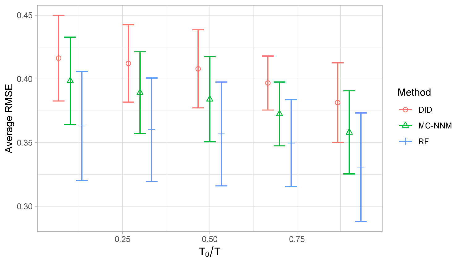
This study adopts the cross-validation scheme of Athey et al. (2021) to compare the DID, MC-NNM, and random forest based on their accuracy in approximating artificially missing fatality rates. The panel dataset for cross-validation uses data from the nonlegalized states selected using the PSM and conventional matching approaches. In this dataset, staggered legalization of marijuana is simulated by randomly selecting three states that would legalize the drug at different times T₀, where the ratio T₀/T takes on the values 0.1, 0.3, 0.5, 0.7, and 0.9. The observations that remained in the nonlegalized group then constitute the training set, while the observations in the legalized group represent the testing set. The methods can be compared based on their accuracy (corresponding to lower RMSE). The procedure of simulating marijuana legalization and estimating RMSEs is repeated 10 times, then average RMSEs and their standard errors are computed.

4. Results

4.1. Canada

The results for the average cost per claim are as follows. The 95% confidence intervals for the effect of marijuana legalization in Canada in the mixed-effects model have centers close to zero, and all versions of the confidence intervals contain zero (Table 2), implying no significant effects on the average cost per claim.

Results for the claim frequency per 100 earned vehicles lead to the same conclusions as the results for the average cost per claim presented in the previous section. Specifically, the 95% confidence intervals for the effect of marijuana legalization in Canada in the mixed-effects model have their centers close to zero, and all versions of the confidence intervals contain zero (Table 2), implying no significant effects.

The results obtained based on quarterly data for Québec matched the ones obtained here based on annual data; the estimated changes in average cost per claim and claim frequency were categorized as not statistically significant (see Appendix).

4.2. United States

4.2.1. Propensity score matching

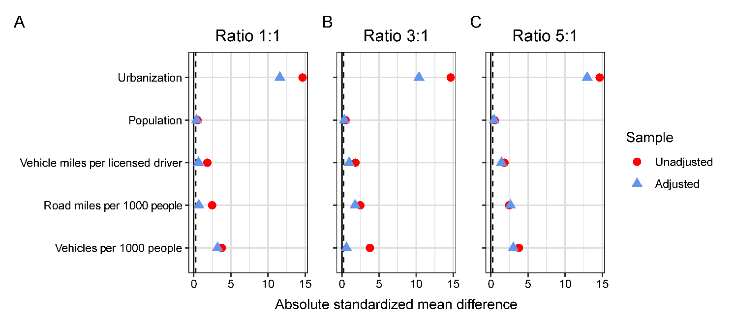
The PSM was done for several alternative ratios of the number of selected control states to the number of legalized states. Based on the absolute standardized mean differences in Figure 3, the best matching is achieved at the ratio 1:1 (the adjusted sample differences, corresponding to the selected controls and legalized states, are the smallest). The effect of matching is still noticeable at the ratio of 3:1, but at the higher ratio of 5:1, the selected control states do not achieve a desirable similarity in the baseline variables (Figure 3). The distribution of propensity scores provides the background information for the observed behaviors. The propensity scores of the treated states (states with legalized marijuana) vary from about 0.15 to 0.30, and there are only a few untreated states with propensity scores in this range. With the PSM algorithm tasked to select more matches for each treated state (as the ratio increases), more states with out-of-range propensity scores around 0 are selected as controls. Table 3 shows the matches for each legalized state.

The 1:1 matching appears to be optimal in this study because it provides substantially more homogeneous samples (Figure 3A) and happens to follow the approach of stratified matching (Damrongplasit, Hsiao, and Zhao 2010) where the control units were selected from the propensity score range of the treated units.

Figure 3.Standardized mean differences for propensity score matching with different ratios of selected control to treated states. The dashed line corresponds to the threshold of 0.25.

4.2.1.1. Conventional matching

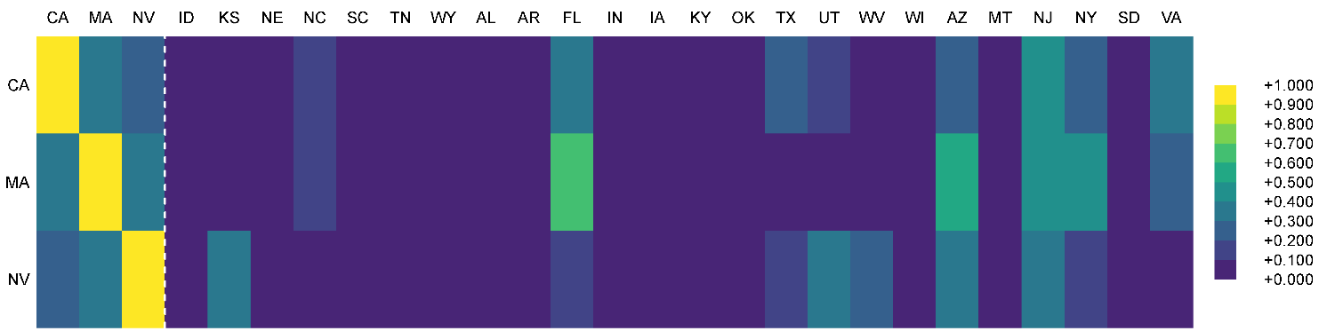
Similarities between states derived from a random forest (Figure 4) were used to find alternative matches. Each state in the Legalized group was matched with the most similar state in the control group if the latter had not been used as a match:

• for the state of California: New Jersey

• for the state of Massachusetts: Florida

• for the state of Nevada: Utah

Figure 4.Random forest similarity matrix based on the five state variables.

The results of the two matching techniques differ quite substantially, hence both versions are considered in the analysis. Note that even if in both cases the distances were derived based on random forests, the random forest implementations differ (supervised random forest for the PSM model (3.5) and unsupervised random forest for the conventional matching).

4.2.2. Cross-validation results

In the cross-validation study, T = 1,400 daily fatality rates from the five selected nonlegalized states (Florida, New Jersey, New York, Utah, and West Virginia) were used to compare accuracy of the estimation methods. The RMSEs calculated for the random forest were generally lower than for the other methods, but not significantly lower (Figure 5). Overall, random forest had the advantage of using the covariates in a nonlinear way to improve estimates of the outcome; however, given the variability across the cross-validation runs and the limited number of these runs, the advantage did not result in significant gains, as seen from the overlapping intervals in Figure 5. Compared to the results in Athey et al. (2021), the MC-NNM did not significantly outperform the simpler DID, but for the sake of space, results from only random forest (RF) and MC-NNM are reported below. Similar to Athey et al. (2021), Figure 5 shows lower RMSE (increasing accuracy) as the ratio T₀/T increases.

Figure 5.Average RMSEs with 95% confidence intervals (±1.96 s.e.(RMSE)) from 10 cross-validation runs for predicting fatality rate in nonlegalized states.

4.2.3. Estimates of the effects

This section summarizes the results of the analysis of the daily average fatality rate and the number of fatal accidents. All rates are calculated using the annual number of registered vehicles in the studied states. The following predictors were considered in the models: Legal (binary variable for marijuana legalization), State (categorical), Month (categorical), Weekday (categorical), Holiday (categorical), Average daily temperature (°C), Average daily temperature range (°C), and Precipitation (millimeters/day).

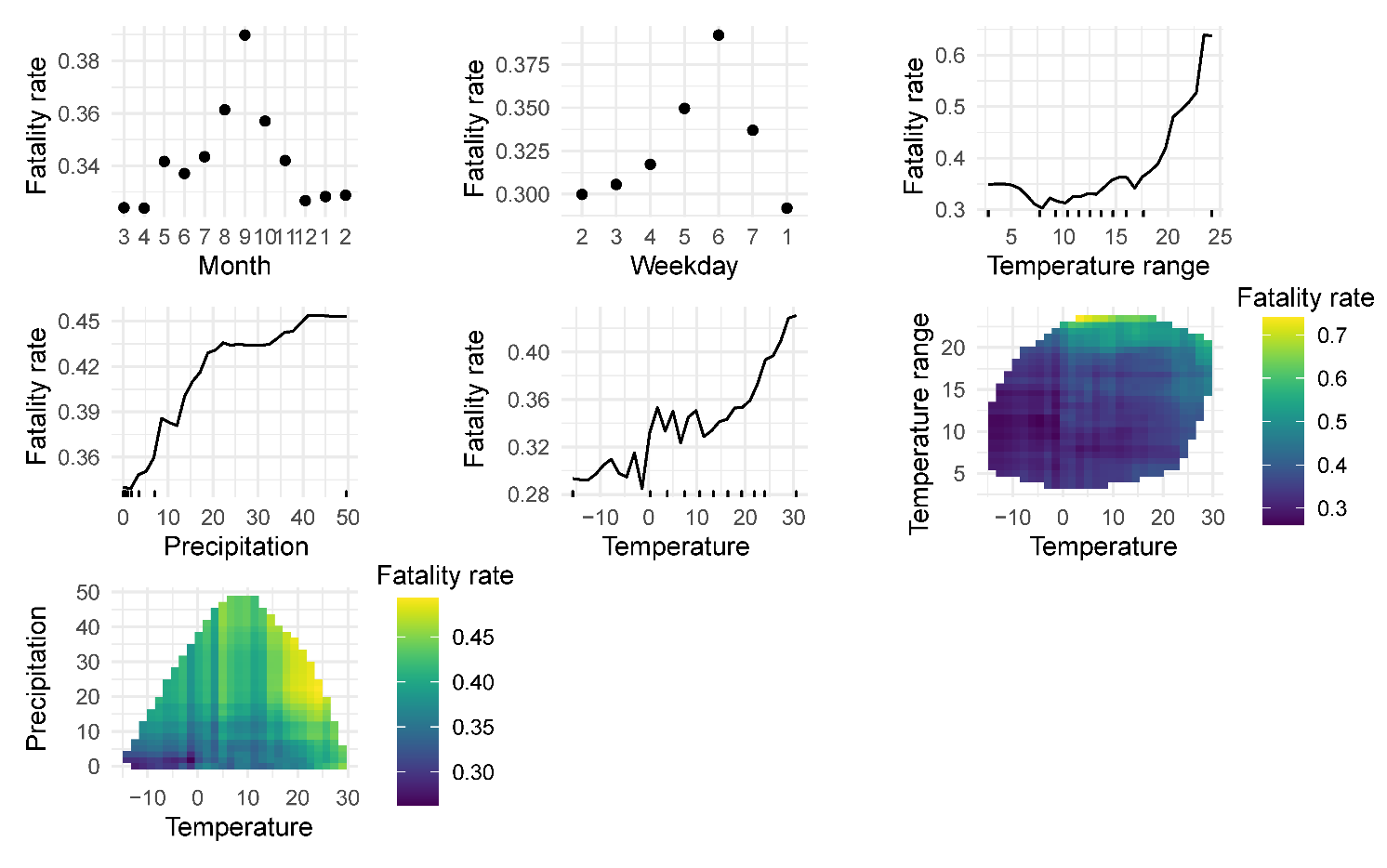
The models were estimated separately for the matched states (mimicking the stratified PSM approach of Damrongplasit, Hsiao, and Zhao 2010) and by combining all selected states, then repeated for the manually matched states. Table 4 summarizes the estimated effects of the legalization; Figure 6 contains PDPs for the fatality rate. (PDPs for the number of fatal accidents are omitted for the sake of space due to the very similar results.)

Figure 6.Partial dependence plots from the random forest model of fatality rate based on all propensity-score-matched states (CA, WV, MA, UT, NV, NY). The inner tick marks on the horizontal axis denote deciles of the corresponding variable; two-dimensional plots are restricted to the convex hull of the observed data to avoid extrapolation.

Based on the random forest results, the effect of legalization is ranked as the least or second-to-least important (another least-important variable is Holiday; the rankings are not shown). The estimated effects show a small not statistically significant decrease, except when comparing Massachusetts and Florida, where the decrease is deemed statistically significant (Table 4). Note that due to the generally large p-values for this variable and the considerable computing time required by the Altmann’s algorithm, only 100 permutations were used to calculate the p-values for random forest. (More permutations can be used to estimate p-values more precisely, but it would not change the conclusions of nonsignificance in those cases where the p-values are already large.)

Based on the MC-NNM results, none of the combinations of states showed significant effects of the legalization (Table 4). The algorithm for selecting the ARMA orders p and q (Hyndman, Athanasopoulos, Bergmeir, et al. 2023) resulted in an ARMA model with zero mean in all of the cases, hence matching the results of the t-test reported in Table 4.

Conclusion and discussion

This study used several data-driven techniques to analyze the effects of marijuana legalization on the vehicle driving experience in Canada and the U.S. The data included frequency and size of auto insurance claims in Canada and road fatalities in the US.

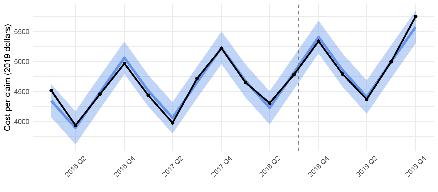
The techniques employed in the study allowed us to account for multiple factors such as weather and similarity of the US states in terms of road and population characteristics. However, the most prominent factors remained the repeating patterns of human activity reflected in seasonal and weekly cycles. Thus, just by looking at a few pre-legalization years in Québec, the trend-seasonal statistical model (termed restricted in this study because it did not use the information on the policy change) was able to accurately predict insurance variables for the next year. Based on the daily aggregated US data, the most predictive factors of the road accidents and fatalities were the state (for regional differences) and day of the week, often followed by temperature and precipitation. PDPs showed increased chances of accidents and fatalities with higher temperatures and, particularly when New York was included in the comparisons via manual matching of the states, also with below-freezing temperatures of around –10°C. The same rankings of the variables were observed for daily data in Mexico City by Bailey, Olivera-Villarroel, and Lyubchich (2020), although that study did not focus on the effects of policy change. The US results varied by the state pair, including the cases when the control state changed. Most of the tests for the legalization effect on fatalities failed to detect a statistically significant change. (Aydelotte, Brown, Luftman, et al. 2017 and Hansen, Miller, and Weber 2020 came to a similar conclusion by analyzing the states of Colorado and Washington.)

Overall, like most other statistical modeling studies, this analysis assumes that the models accounted for all potential confounders that could affect the inference about the effects of legalization. For example, the study accounted for the effects of weather and deliberately did not use the period of the COVID-19 pandemic. However, there could be other effects one may want to control, such as new legislation about driving, traffic control practices, road and other infrastructure development, and adoption of AI-enabled features in vehicles. These factors will become particularly important if one wants to extend the period of the study.

Another important aspect when deciding on the study period is the speed of adoption. There has always been some time between the legalization and the start of sales, and even then, one should not assume that all potential consumers start using marijuana at once. The short-term effects detected by Lane and Hall (2019) might be an exception to this rule since they were observed in the early-adopter states and could be explained by the high anticipation by residents and even visitors looking forward to consuming marijuana. This study used at least a year of records after the start of commercial sales in each case, but some may argue that the effects take even longer to surface due to the time needed for the new market to develop (e.g., to open more dispensaries, run marketing campaigns, and adjust prices). For example, Smart and Doremus (2023) point out increases in youth marijuana use associated with the legal market growth and increased availability of the drug.

There are other open questions in marijuana-related research, related to the ways people perceive the drug, recognize different levels of tolerance, and get tested for being influenced by the drug. The history of public health crises linked to tobacco, alcohol, and opioids understandably raises concerns about marijuana legalization (DeVillaer 2019). Some research suggests a potential cannabis–alcohol substitution effect, with a decrease in alcohol-related accidents due to marijuana use primarily at home (Ellis et al. 2022). However, concerns exist regarding potential underestimation of addiction risks compared to alcohol and tobacco (Ammerman et al. 2015). Finally, post-accident THC testing is not yet as effective as alcohol testing (Alexander 2003). Recent studies by Brands, Di Ciano, and Mann (2021) and Preuss, Hoch, and Wong (2023) highlight ongoing research areas, including the dose–response relationship (e.g., concentration of THC in blood and actual driving behavior, or uncertainty about which THC concentration consistently results in impairment); tolerance after frequent use; effects of cannabidiol (CBD) to THC ratios; and different consumption methods (e.g., smoking, vaping, or edibles).

Acknowledgments

The author thanks the project oversight group composed of Qi An, Caryn Carmean, Brian Fannin, Aditya Khanna, Harsha Maddipati, and Marc-Olivier Menard, along with the Canadian Institute of Actuaries and Casualty Actuarial Society for their support in developing the project.