Pricing Cyber Risks Over Modern Networks via Bayesian Attack Graphs

1. Introduction

Cyber risk has emerged as one of the most significant threats in the digital age. Cyber attacks may have severe consequences, such as exposure of sensitive information, identity fraud, and substantial financial losses. The sophistication of modern cyber attacks often outpaces protective measures, as evidenced by the increasing number of data breaches organizations have recently experienced. For instance, the Privacy Rights Clearinghouse reported 18,353 data breaches between 2010 and 2021, resulting in nearly 1.5 billion breached records (Privacy Rights Clearinghouse, n.d.). The Identity Theft Resource Center and Cyber Scout reported a significant increase in data breach incidents in 2022, exposing over 422 million records, a stark rise from the nearly 294 million records exposed in 2021 (Identity Theft Resource Center, n.d.). The financial implications of these breaches are substantial. According to NetDiligence, small-to-medium enterprises (i.e., those with less than $2 billion in annual revenue) faced an average breach cost of $170,000, excluding an average crisis service cost of $110,000 and an average legal cost of $82,000. For larger companies (i.e., those with $2 billion or more in annual revenue), the average breach cost rose to $15.4 million, with an average crisis service cost of $4.1 million and a legal cost of $3.1 million (NetDiligence, n.d.). Cybersecurity Ventures expects global cybercrime costs to grow by 15% per year over the next few years, reaching US$10.5 trillion annually by 2025.^[1]

In traditional centralized networks, vulnerabilities can often be mitigated through patches and upgrades to the operating systems. However, modern networks, particularly those incorporating Internet of Things devices with lightweight operating systems and limited computational capabilities, present unique challenges. It is not always possible to identify and patch vulnerabilities in these networks, making risk assessment and prioritization essential for optimizing resource allocation and protective efforts. However, analyzing network risks in isolation provides a limited perspective on network security owing to the complex interdependency between vulnerabilities. In this context, Bayesian Attack Graphs (BAGs; Koller and Friedman 2009) offer a powerful framework for representing prior knowledge about vulnerabilities and network connectivity, which can illustrate the potential paths an attacker could take through the system by exploiting successive vulnerabilities.

Our study objective was to develop a practical probabilistic approach for pricing cyber risks in modern networks using BAGs. BAGs are graphical models that represent knowledge about network vulnerabilities and their interactions, illustrating the various paths an attacker can take to compromise a given objective by exploiting a set of vulnerabilities (Poolsappasit, Dewri, and Ray 2011). Each attack path involves a sequence of exploited vulnerabilities, with each successful exploit granting the attacker additional privileges toward their goal. Modeling cyber risk using BAGs has been a recurrent theme in the literature, predominantly within the realm of cybersecurity. For instance, Poolsappasit, Dewri, and Ray (2011) proposed a risk management framework that leverages BAG, allowing system administrators to quantify the likelihood of network compromise across static risk assessment, dynamic risk assessment, and risk mitigation analysis. Muñoz-González et al. (2017) delved into belief propagation and junction tree algorithms for exact inferences in BAGs, focusing on static and dynamic network risk assessments. Sun et al. (2018) pioneered a probabilistic approach with the ZePro system, which was designed for zero-day attack path identification and demonstrates the efficacy of BAG in revealing such paths. d’Ambrosio, Perrone, and Romano (2023) extended the applicability of BAG to insider threats, formulating a Bayesian Threat Graph for cyber risk management. Kim et al. (2023) proposed adaptive moving target defense operations based on BAG analysis that uses a knapsack problem to optimize vulnerability reconfiguration in software-defined networking. In the field of actuarial science, however, the use of BAG for insurance pricing remains relatively limited. Noteworthy contributions include Shetty et al. (2018), who developed a cyber risk assessment method based on BAG to address the challenges posed by the absence of historical data and the dynamic nature of cyber risk. While they focused on estimating attack probabilities through asset-at-risk monitoring and continuous software vulnerability scoring, their work leaned toward descriptive rather than probabilistic modeling. Tatar et al. (2020) presented a probabilistic framework for assessing enterprise cyber risk using BAG to compute attack likelihoods based on scenario examples.

Two key aspects distinguish our work from existing studies. First, we focus on modern networks, presenting a practical methodology to identify vulnerabilities and estimate exploit probabilities. Second, we introduce a novel top-down approach for computing joint exploit probabilities, departing from the conventional variable elimination algorithm prevalently employed in the studies mentioned earlier. Further, our contribution extends to exploring pricing strategies based on BAG analysis, a dimension yet unexplored in the current literature. Our contributions are summarized as follows:

• Practical approach for identifying and characterizing cyber risks in modern networks: We propose a practical method to identify and characterize cyber risks in a modern network. This involves detailing the modern network and the vulnerabilities present in network devices, including reports from vulnerability scanners (Walkowski et al. 2020), vulnerability dependency details, and scores assigned to the vulnerabilities by standards such as the Common Vulnerability Scoring System (CVSS; “Common Vulnerability Scoring System,” n.d.) and the Exploit Prediction Scoring System (EPSS; Jacobs et al. 2023). These details are abstracted into a vulnerability graph for modeling purposes.

• Modeling cyber risks in modern networks via BAGs: We formulate the nodes of the graph as device vulnerabilities and the edges as vulnerability dependencies. We identify potential attack initiation points in the network and model them as source nodes. Similarly, potential target points, toward which attacks may be directed, are identified and modeled as sink nodes. We analyze the abstracted vulnerability graph via the BAG and propose a novel top-down approach to compute the joint exploit probability across the network.

• Cyber insurance pricing: We explore various cyber insurance pricing strategies based on the exploit probabilities within the modern network. Through a simulation study, we scrutinize these strategies, perform sensitivity analysis, and discuss the impact of dependence on the insurer.

2. A quantitative framework for modeling and pricing cyber risks over modern networks

Despite the growing importance of cyber risk management, few studies have modeled cyber risks in modern networks from an insurer’s perspective. Our study presents a quantitative framework for modeling and pricing cyber risks within a modern network. This framework comprises three key components: (1) identifying vulnerabilities that incur cyber risks, (2) modeling cyber risks and computing compromise probabilities, and (3) determining premiums.

2.1. Identifying and characterizing cyber risks in modern networks

Modern networks, with their inherent complexity and heterogeneous structure, present a large attack surface (Denning, Kohno, and Levy 2013; Davis, Mason, and Anwar 2020). From an insurer’s perspective, it is crucial to identify these risks using a simple yet efficient approach. To this end, we propose identifying risks based on vulnerabilities present in a modern network.

A common approach to assessing vulnerability primarily relies on the CVSS, which calculates the severity of a vulnerability based on its characteristics and the impact on an information system’s confidentiality, integrity, and availability. The CVSS base score, which ranges from 0 to 10, is the most commonly used component, with a higher score indicating a higher threat level. Almost all known vulnerabilities are published on the National Vulnerability Database’s website.^[2] Each vulnerability, identified via common vulnerabilities and exposures (CVE), includes the CVE identifier, description, and references discussing the vulnerability. However, it is important to note that the CVSS score does not reflect the probability of a vulnerability being exploited in an attack, since only a small proportion of vulnerabilities are exploited in practice. Therefore, it is necessary to convert the CVSS into an exploitation probability. Jacobs et al. (2021) proposed a data-driven framework, the EPSS,^[3] for assessing the probability that a vulnerability will be exploited within a certain period after public disclosure.

To identify cyber risks in modern networks, we first identify the exploitable elements in the network and the devices in which they reside. These exploitable elements are associated with the network because of inherent vulnerabilities in different network devices. Attackers may concatenate these exploitable elements to form channels to reach critical resources in the network. This identification can be completed via vulnerability scanners (Walkowski et al. 2020). Further, the network details, including topology, configuration, connectivity among devices, and access control policies, are used to create the vulnerability graph.

The following are performed to identify cyber risks in modern networks:

1. Scan vulnerabilities: Typically, the vulnerability report generated by vulnerability scanners includes vulnerability dependency details and CVSS scores (Walkowski et al. 2020).

2. Create the vulnerability graph: The vulnerability graph is created based on the vulnerability details.

3. Determine exploitation probabilities: Vulnerabilities’ exploitation probabilities can be determined from the vulnerability graph based on vulnerability details.

For illustration, consider a smart home network with three discovered vulnerabilities: CVE-2021-21736 ($V_1$), CVE-2018-3919 ($V_2$), and CVE-2022-22667 ($V_3$). The vulnerability graph is created based on the attack scenario: the attacker exploits a vulnerability in a smartphone operating system (CVE-2022-22667) over the wireless network and compromises the smartphone. This grants the attacker access to the operating system, which allows the attacker to pivot into the smart home network to compromise the smart home hub by exploiting the vulnerability (CVE-2018-3919). Further, the attacker exploits the vulnerability (CVE-2021-21736) in the smart camera to gain control over it. The vulnerability graph can be represented as a path of two edges, $$V_{3}\rightarrow V_{2} \rightarrow V_1.$$ The CVSS base scores for these vulnerabilities are 7.8 ($V_{3}$), 9.9 ($V_2$), and 7.2 ($V_1$). The EPSS probabilities are $.02$, $.3$, and $.05$, respectively. This example illustrates how vulnerabilities in a modern network can be identified, characterized, and graphically represented, providing a basis for assessing and pricing cyber risks.

2.2. Modeling the cyber risks in modern networks via BAGs

This section discusses how to model the risk over a modern network via BAGs and develops a new approach to compute the compromise probability.

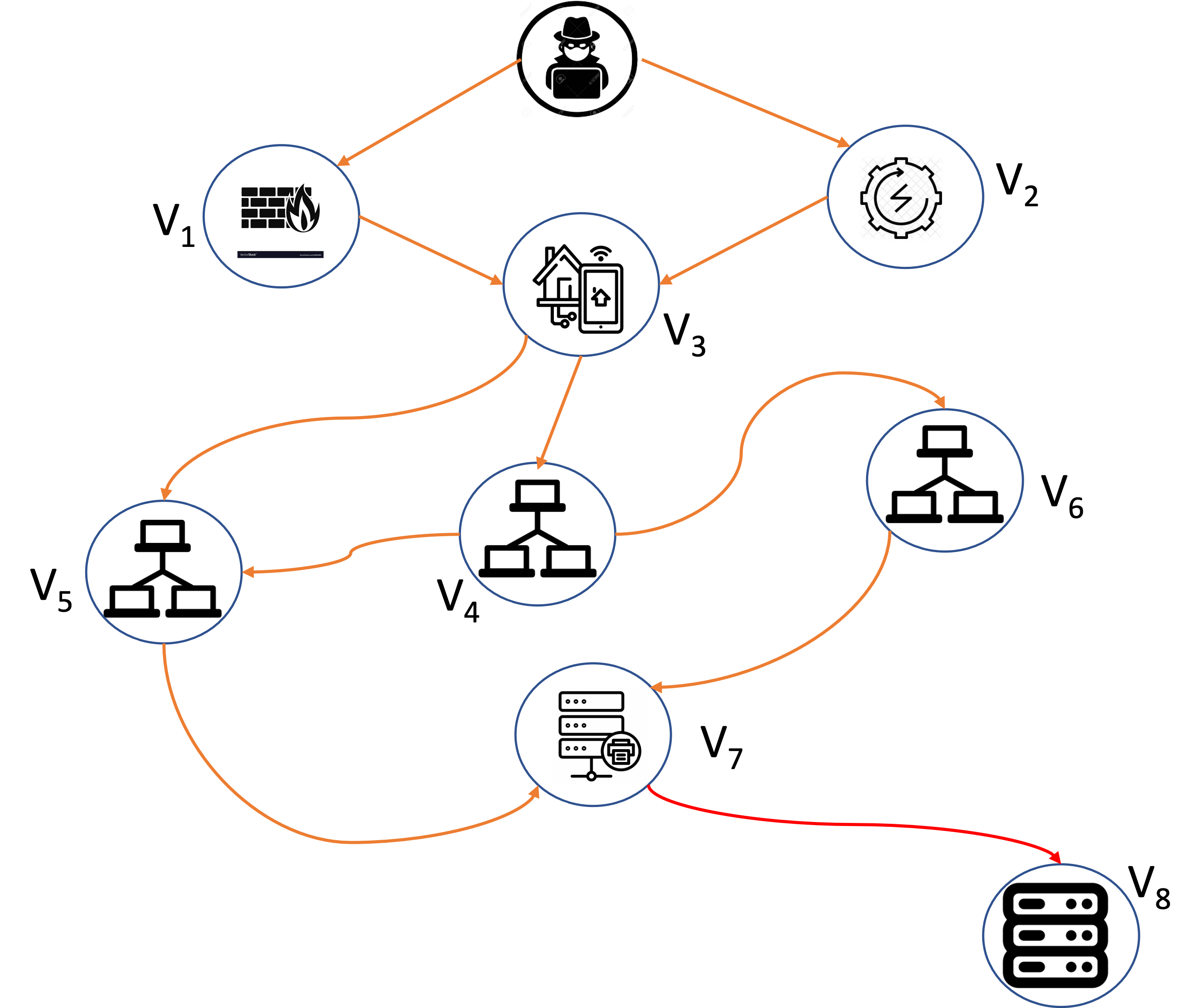
Let $G(V,E)$ represent the vulnerability graph over a modern network, where $V=\{V_1,V_{2},\ldots,V_N\}$ is the set of vulnerabilities with size $N=|V|$, and $E=\{E_{ij}: i,j \in V\}$ is the set of edges. Note that node $V_{i}$ represents vulnerability $i$ in the network, and edge $E_{ij}$ represents the possibility of exploitation from vulnerability $i$ to vulnerability $j$. Figure 1 illustrates a modern industrial network with the graphical representation of vulnerability relations.

Figure 1.Illustration of an exploitable vulnerability network graph.

We consider two possible attack scenarios:

• Attack scenario 1: The attacker exploits the firmware vulnerability ($V_{1}$: CVE-2017-9861) in the network and compromises it. This grants the attacker access to the local operating system. The attacker can use this access to pivot into the internal network and further compromises the building management system in the network by exploiting the vulnerability ($V3$: CVE-2012-4701). Further, the attacker exploits the vulnerability ($V_{4}$: CVE-2013-0640) in the LAN user machine to obtain limited privileges in the machine. The attacker then exploits a privilege escalation vulnerability ($V_{5}$: CVE-2017-11783) to gain local admin privileges on the same machine. The attacker uses the directory traversal vulnerability ($V_{7}$: CVE-2008-0405) to access unauthorized files in the file and print server. The password vulnerability of the central server ($V_{8}$: CVE-2010-2772) can be exploited via the file and print server to compromise and control the whole system, which can cause catastrophic financial losses. The attack path can be represented via edges as $E_{13}\rightarrow E_{34}\rightarrow E_{45}\rightarrow E_{57}\rightarrow E_{78}$.

• Attack scenario 2: The attacker exploits the vulnerability ($V_{2}$: CVE-2017-9859) in the inverter unit of the building power management and then exploits the vulnerability ($V3$: CVE-2012-4701) in the building management system. The attacker can further exploit the vulnerability ($V_{4}$: CVE-2013-0640) in the LAN user machine and attack the vulnerability ($V_{6}$: CVE-2013-0640). After that, an attack is further launched into the file and print server through the vulnerability ($V_{7}$: CVE-2008-0405). Then, the password vulnerability of the central server ($V_{8}$: CVE-2010-2772) can be exploited. This attack path can be represented via edges as $E_{23}\rightarrow E_{34}\rightarrow E_{46}\rightarrow E_{67}\rightarrow E_{78}$.

Let $V_{j}$ be a random variable representing vulnerability$j$, and $X_{j}$ represent the associated loss with the exploited vulnerability $j$. Then, the total loss can be presented as

$$L=\sum_{j=1}^{N} L_j= \sum_{j=1}^{N} {\rm I}(V_j) X_{j},$$

where ${\rm I}(\cdot)$ is the identity function and $L_j={\rm I}(V_j) X_{j}$ is the loss associated with the exploited vulnerability $j$. Note that the joint probability of vulnerabilities can be represented via BAG as

$$\begin{aligned} P(V_{1} & =v_{1},\ldots, V_{N}=v_{N})=\prod_{i=1}^{N}P(V_{i}=v_{i}|{\bf pa}_{i}),\\ \quad v_{i} &=1,0, \end{aligned}$$

where ${\bf pa}_{i}$ is the parent node set of vulnerability node $i$ (e.g., vulnerability node $V_{5}$ in Figure 1 has the parent node set ${\bf pa}_{5}=\{V_{3},V_{4}\}$) and

$$v_{i}= \left\{ \begin{array}{cc} 1,& {\rm Compromised,} \\ 0, & {\rm Otherwise.} \end{array} \right.$$

For example, in Figure 1, we have

$$\begin{aligned} & P(V_1, V_2, V_3, V_4, V_5, V_6, V_7, V_8)\\ = &P(V_1)P(V_2)P(V_3|V_1,V_2)P(V_4|V_3)\\ & \ \cdot P(V_5|V_3,V_4)P(V_6|V_4)P(V_7|V_5,V_6)P(V_8|V_7). \end{aligned}\tag{1}$$

Note that the conditional exploitation probability of $V_{j}$ can be represented as

$$\small{\begin{aligned} e_{j} &= P(V_{j}=1|{\bf pa}_{j})\\ & =\left\{ \begin{array}{cc} 0 &\forall V_i \in {\bf pa}_{j}, V_i=0; \\ 1-\prod_{V_i \in {\bf pa}_{j}, V_i=1}(1- e_{ij}), & \mbox{Otherwise} \end{array} \right. \end{aligned}}\tag{2}$$

where $e_{ij}=P(V_{j}=1|V_{i}=1)$. Computing the compromise probability is challenging because it involves many possible attack paths and is an NP-Hard problem. In the literature, an effective approach for computing the exploitation probability is known as the variable elimination (VE) algorithm (Liu and Man 2005; Muñoz-González et al. 2017; Koller and Friedman 2009). This approach identifies a small number of variables to compute the joint distribution and avoids generating them exponentially many times.

To illustrate, we use the VE approach to calculate the probability $P(V_6=1)$ using the following elimination ordering: $V_1\rightarrow V_2\rightarrow V_3\rightarrow V_4\rightarrow V_5\rightarrow V_7\rightarrow V_8$. The step-by-step procedure is as follows:

1. Eliminating $V_1$: We evaluate the expression

   $$\begin{aligned} & \tau_{V_1}(V_2=v_2,V_3=v_3)\\ = & \sum_{v_1=0}^1 P(V_1=v_1)P(V_3=v_3 | V_1=v_1, V_2=v_2),\end{aligned}$$

   where $v_2,v_3\in \{0,1\}$.

2. Eliminating $V_2$: We derive the equation

   $$\begin{aligned} & \tau_{V_2}(V_3=v_3)\\ = & \sum_{v_2=0}^1 \tau_{V_1}(V_2=v_2,V_3=v_3)P(V_2=v_2).\end{aligned}$$

3. Eliminating $V_3$: We calculate

   $$\scriptsize{\begin{aligned} & \tau_{V_3}(V_4=v_4,V_5=v_5)\\ = &\sum_{v_3=0}^1 \tau_{V_2}(V_3=v_3)P(V_4=v_4|V_3=v_3)P(V_5=v_5|V_3=v_3,V_4=v_4),\end{aligned}}$$

   where $v_4,v_5\in \{0,1\}$.

4. Eliminating $V_4$: We use the expression

   $$\begin{aligned} & \tau_{V_4}(V_5=v_5,V_6=1)\\ = & \sum_{v_4=0}^1 \tau_{V_3}(V_4=v_4,V_5=v_5) P(V_6=1|V_4=v_4).\end{aligned}$$

5. Eliminating $V_5$: We determine

   $$\small{\begin{aligned} & \tau_{V_5}(V_6=1,V_7=v_7)\\ = & \sum_{V_5} \tau_{V_4}(V_5=v_5,V_6=1) P(V_7=v_7|V_5=v_5,V_6=1),\end{aligned}}$$

   where $v_7\in \{0,1\}$.

6. Eliminating $V_7$: We compute

   $$\begin{aligned} & \tau_{V_7}(V_6=1,V_8=v_8)\\ = & \sum_{v_7=0}^1 \tau_{V_5}(V_6=1,V_7=v_7) P(V_8=v_8|V_7=v_7),\end{aligned}$$

   where $v_8\in \{0,1\}$.

7. Eliminating $V_8$: Finally, we obtain

   $$P(V_6=1)=\sum_{v_8=0}^1 \tau_{V_7}(V_6=1,V_8=v_8).$$

It is important to note that the VE approach is essentially a bottom-up method for computing the exploitation probability, as it consistently considers the parent nodes and eliminates all other nodes except the one of interest. In the subsequent section, we present a top-down approach for computing the joint exploitation probability, which draws inspiration from the back elimination (BE) approach introduced in Da et al. (2020).

Theorem 2.1. Let $G(V,E)$ be the vulnerability graph of a modern network. Assume that target node vector $V^0=(V_{i_1},\ldots, V_{i_l})$ does not include any leaf node,^[4] then it holds that,

$$\scriptsize{\begin{aligned} &P(V_{i_1}=\ldots= V_{i_l}=1)\nonumber\\ =& \sum_{D_0 \subset D_{\rm leaf}} \sum_{L=1}^{\hat{L}} \left(\sum_{D_{L-1} \subset V \setminus \left( D_0 \cup D_1 \cup \cdots \cup D_{L-2} \right) } \cdots \sum_{D_1 \subset V \setminus D_0 } \right. \nonumber\\ &P\left(\left(\left(V_{i_1}=\ldots= V_{i_l}\right)\setminus \left(D_{L-1}\cup\cdots\cup D_0\right)\right)=\mathbf{1},1|D_{L-1}\right)\\ & \prod_{j=0}^{L-2} P(D_{j+1},1|D_{j}) \bigg) P(D_0) \end{aligned}}\tag{3}$$

where ${\hat{L}}$ is the longest path of the BAG.

$$P(D_0)=\prod_{i\in D_0} p_i \prod_{D_{\rm leaf} \setminus {D}_0} (1-p_i),$$

where $D_0 \subset D_{\rm leaf}$, $D_{\rm leaf}$ represents the set of leaf nodes, and $p_i$ is the outside compromise probability for node $i$.

$$\begin{aligned}P(D_L,1|D_{L-1}) &=\prod_{j \in D_{L}} (1-\prod_{i \in D_{L-1}} (1-e_{ij} \alpha_{ij}) ) \\ & \quad \cdot \prod_{j \in \overline{D_0 \cup \cdots \cup D_{L} }} \prod_{i \in D_{L-1}} (1-e_{ij}\alpha_{ij})\end{aligned}$$

where $e_{ij}=P(V_j=1|V_i=1)$ and $(\alpha_{ij})$ is the adjacent matrix of the BAG.

Proof: Let $D_0$ be the set of originally compromised nodes chosen from leaf nodes $D_{\rm leaf}$ in BAG. Then, we have

$$\begin{aligned} P(V^0=\mathbf{1})=\sum_{D_0\subset D_{\rm leaf}}P(V^0=\mathbf{1}|D_0)P(D_0), \end{aligned}$$

where

$$P(D_0)=\prod_{i\in D_0} p_i \prod_{D_{\rm leaf} \setminus {D}_0} (1-p_i),$$

and $p_i$ is the outside compromise probability for node $i$. Assume that $L$ is the number of steps needed to reach all the targets. Thus, we have

$$\begin{aligned} P(V^0=\mathbf{1},L|D_0)=P(V^0\setminus D_0=\mathbf{1},L|D_0). \end{aligned}$$

Let $D_1 \subset V \setminus D_0$ be the set of compromised nodes in the first step. Denote $V^1=V^0\setminus D_0$. Then, we have

$$\begin{aligned} & P(V^1=\mathbf{1},L|D_0)\\ = & \sum_{D_1 \subset V \setminus D_0} P(V^1=\mathbf{1},L|D_1,D_0)P(D_1,1|D_0)\\ = & \sum_{D_1 \subset V \setminus D_0} P(V^1=\mathbf{1}, L-1|D_1)P(D_1,1|D_0)\\ = & \sum_{D_1 \subset V \setminus D_0} P((V^1 \setminus D_1)=\mathbf{1}, L-1|D_1)P(D_1,1|D_0). \end{aligned}$$

The second equation holds because given $D_0$ and $D_1$, the status of $\{V^1=\mathbf{1}\}$ only depends on $D_1$. As a result, we can eliminate $D_0$ from the BAG, and $L$ is reduced by 1. Using a similar argument, denote $V^2=V^1 \setminus D_1$, it holds that

$$\begin{aligned} &P(V^2,L-1|D_1)\\ =&\sum_{D_2 \subset V \setminus \left( D_0 \cup D_1 \right)} P(V^2=\mathbf{1},L-1|D_2,D_1)P(D_2,1|D_1)\\ =&\sum_{D_2 \subset V \setminus \left( D_0 \cup D_1 \right)} P(V^2=\mathbf{1},L-2|D_2)P(D_2,1|D_1)\\ =&\sum_{D_2 \subset V \setminus \left( D_0 \cup D_1 \right)} P((V^2 \setminus D_2=\mathbf{1},L-2|D_2)P(D_2,1|D_1). \end{aligned}$$

By applying the same iterative argument, we have the following explicit expression:

$$\begin{aligned} &P(V_{i_1}=\ldots= V_{i_l}=1)\nonumber\\ =& \sum_{D_0 \subset D_{\rm leaf}} \sum_{L=1}^{\hat{L}} \left(\sum_{D_{L} \subset V \setminus \left( D_0 \cup D_1 \cup \cdots \cup D_{L-1} \right) } \cdots \sum_{D_1 \subset V \setminus D_0 } \right. \nonumber\\ & P((V^{L-1}\setminus D_{L-1})=\mathbf{1},1|D_{L-1})P(D_{L-1},1 |D_{L-2})\\ & \cdots P(D_2, 1 |D_1)P(D_1, 1 |D_0)\bigg)P(D_0), \end{aligned}$$

where

$$\begin{aligned} P(D_L,1|D_{L-1}) &= \prod_{j \in D_{L}} (1-\prod_{i \in D_{L-1}} (1-e_{ij} \alpha_{ij}) )\\ & \quad \cdot \prod_{j \in \overline{D_0 \cup \cdots \cup D_{L} }} \prod_{i \in D_{L-1}} (1-e_{ij}\alpha_{ij}), \end{aligned}$$

and $e_{ij}=P(V_j=1|V_i=1)$ can be obtained from the EPSS and $(\alpha_{ij})$ is the adjacent matrix of the BAG.

For illustration and comparison, we employ Theorem 1 to calculate the probability $P(V_6=1)$ in Figure 1. The network can only be compromised through $D_{\rm leaf}=\{V_1, V_2\}$, implying that $D_0\subset\{V_1,V_2\}$. In the following discussion, we focus on the scenario where $D_0=\{V_1\}$, while the other cases can be similarly analyzed. When $D_0=\{V_1\}$, the next compromised node can only be $D_1=\{V_3\}$. Notably, given $D_1=\{V_3\}$, the value of $P(V_6=1)$ does not depend on $D_0$. Consequently, we have $D_2\subset\{ V_4,V_5 \}$.

• If $D_2=\{V_4,V_5\}$, the value of $P(V_6=1)$ is no longer influenced by $D_1$. Consequently, in the third step, node $V_4$ can compromise $V_6$. As per Theorem 1, the probability of this event is given by:

  $$\begin{aligned} & P(D_0=\{V_1\})P( D_1=\{ V_3 \} |D_0=\{ V_1 \})\\ & \cdot P( D_2=\{ V_4, V_5 \} |D_1=\{ V_3 \})\\ & \cdot P( V_6=1|D_2=\{ V_4, V_5 \}).\end{aligned}$$

• If $D_2=\{ V_4 \}$, the value of $P(V_6=1)$ is no longer influenced by $D_1$. Consequently, in the third step, node $V_4$ can compromise $V_6$. As per Theorem 1, the probability of this event is given by:

  $$\begin{aligned} & P(D_0=\{V_1\})P( D_1=\{ V_3 \} |D_0=\{ V_1 \})\\ & \cdot P( D_2=\{ V_4\} |D_1=\{ V_3 \})\\ & \cdot P( V_6=1|D_2=\{ V_4 \}).\end{aligned}$$

• If $D_2=\{ V_5 \}$, the value of $P(V_6=1)$ is no longer influenced by $D_1$. However, in the third step, node $V_5$ cannot directly compromise $V_6$. As a result, according to Theorem 1, the probability of this event is:

  $$\begin{aligned} & P(D_0=\{V_1\})P( D_1=\{ V_3 \} |D_0=\{ V_1 \})\\ & \cdot P( D_2=\{ V_5\} |D_1=\{ V_3 \})\\ & \cdot P( V_6=1|D_2=\{ V_5 \})\\ = & 0.\end{aligned}$$

For the cases of $D_0=\{ V_2\}$ and $D_0=\{ V_1,V_2 \}$, the resulting next step is $D_1=\{V_3\}$ in both cases, and the subsequent steps follow the same discussion as above. Consequently, the probability $P(V_6=1)$ can be obtained. The new BE approach is a top-down method compared with VE, as it consistently identifies the offspring nodes and eliminates nodes along the attack path without the need to eliminate unrelated nodes such as $V_7$ and $V_8$.

Table 1 presents the probability of compromise for each $V_i$, where $i=3,\ldots,8$, when $P(V_1)=0.1$, $P(V_2)=0.2$, and $e_{ij}=0.1$ for $i,j=1,\ldots, 8$, using the explicit formula derived from Theorem 1 as well as through 1,000,000 simulations. The results obtained from Theorem 1 align perfectly with the outcomes of the simulations, affirming their consistency and reliability.

We can also use Theorem 1 to calculate the compromise probability between any two vulnerabilities. However, for the sake of simplicity, Table 2 presents only the compromise probabilities between $V_3$ (or $V_5$) and $V_i$s. Once again, we observe that the calculated probabilities and the simulated probabilities are very close.

Comparison between VE and BE. Compared with the VE approach, the proposed BE approach confers the following advantages.

• Expandability. The BE approach efficiently computes compromise probabilities when new vulnerabilities surface, leading to the expansion of the BAG. For illustration, assume that there is a newly discovered vulnerability $V_9$, which only connects to $V_6$ as the parent node in Figure 1. Then Eq. (1) changes to

  $$\begin{aligned} & P\left(V_1, V_2, V_3, V_4, V_5, V_6, V_7, V_8, V_9\right) \\ = & P\left(V_1\right) P\left(V_2\right) P\left(V_3 \mid V_1, V_2\right) P\left(V_4 \mid V_3\right)\\ & \cdot P\left(V_5 \mid V_3, V_4\right) P\left(V_6 \mid V_4, V_9\right)\\ & \cdot P\left(V_7 \mid V_5, V_6\right) P\left(V_8 \mid V_7\right) P(V_9). \end{aligned}$$

  To compute the probability of $V_6=1$ with elimination ordering: $V_1\rightarrow V_2\rightarrow V_3\rightarrow V_4\rightarrow V_5\rightarrow V_7\rightarrow V_8\rightarrow V_9$, as mentioned previously, the VE approach requires recalculating from step (iv) to step (vii) and adding one more step for $V_9$. That is,

• iv*) Eliminating $V_4$: We use the expression

  $$\small{\begin{aligned} & \tau^\ast_{V_4}(V_5=v_5,V_6=1,V_9=v_9)\\ = & \sum_{v_4=0}^1 \tau_{V_3}(V_4=v_4,V_5=v_5) P(V_6=1|V_4=v_4,V_9=v_9).\end{aligned}}$$

• v*) Eliminating $V_5$: We determine

  $$\small{\begin{aligned} & \tau^\ast_{V_5}(V_6=1,V_7=v_7,V_9=v_9)\\ = & \sum_{V_5=0}^1 \tau^\ast_{V_4}(V_5=v_5,V_6=1,V_9=v_9) P(V_7=v_7|V_5=v_5,V_6=1),\end{aligned}}$$

  where $v_7\in \{0,1\}$.

• vi*) Eliminating $V_7$: We compute

  $$\small{\begin{aligned} & \tau^\ast_{V_7}(V_6=1,V_8=v_8,V_9=v_9)\\ = & \sum_{v_7=0}^1 \tau^\ast_{V_5}(V_6=1,V_7=v_7,V_9=v_9) P(V_8=v_8|V_7=v_7),\end{aligned}}$$

  where $v_8\in \{0,1\}$.

• vii*) Eliminating $V_8$: We have

  $$\begin{aligned} & \tau_9(V_6=1,V_9=v_9)\\ = & \sum_{v_8=0}^1 \tau^\ast_{V_7}(V_6=1,V_8=v_8,V_9=v_9).\end{aligned}$$

• viii*) Eliminating $V_9$: Finally, we obtain

  $$P(V_6=1) = sum_{v_9=0}^1 \tau_9 ( V_6=v_6, V_9=v_9 )P(V_9=v_9).$$

  Conversely, the BE approach does not need to be recalculated because it is based on attack paths. We only need to compute the probabilities of newly generated attack paths with $D_0=\{V_9\}$, $D_0=\{V_1,V_9\}$, $D_0=\{V_2,V_9\}$, or $D_0=\{V_1, V_2,V_9\}$. Further, if $V_9$ cannot be exploited from outside, the exploit probability of $V_6$ does not change, which can be seen directly from the BE approach.

• Interpretability. The BE approach offers the attack path interpretability and computational convenience by eliminating the need to consider unrelated nodes, which streamlines the calculation process. For illustration, assume that we are interested in $P(V_5=1)$ in Figure 1. The VE approach requires repeating steps (i)–(vii) to eliminate $V_1$ to $V_8$ except for $V_5$ and to recalculate the newly generated $\tau$ functions. In essence, VE requires considering all conceivable states of vulnerabilities, excluding the targeted $V_5$. Conversely, the BE approach simplifies this process by selectively eliminating vulnerabilities in tandem with attack paths, as delineated in Table 3. To illustrate, upon establishing $D_0=\{V_1,V_2\}$ and $D_1=\{V_3\}$, the BE approach efficiently omits $D_0$ elimination since it has no bearing on the state of $V_5$. Analogously, subsequent elimination of $D_{2}=\{ V_4 \}$ follows, paving the way for calculating the compromise probability of $V_5$ based on $V_4$. This highlights the interpretability of the computational process within the BE approach. Note that the state of $V_6$, $V_7$, and $V_8$ need not be considered, further facilitating the computational efficiency of the BE approach.

In summary, the BE approach not only efficiently incorporates new vulnerabilities but also enhances interpretability by focusing on attack paths, leading to a more streamlined computational process compared with the VE approach. The R script of the computation based on Theorem 1 is available upon request.

We acknowledge that implementing the BE approach may pose challenges when dealing with an excessively large BAG. To illustrate this point, consider the construction of a 15-node BAG by introducing an additional $V_9$ to $V_{15}$ in Figure 1, preserving the same structure as $V_1$ to $V_7$ and connecting $V_{15}$ to $V_8$. Further complexity is introduced by adding another set of nodes, creating a 22-node BAG with the inclusion of $V_{16}$ to $V_{22}$, similarly structured to the 15-node BAG. In practical terms, the time required to compute $P(V_6=1)$ rises from 0.331 seconds for the 15-node BAG to 0.734 seconds and rises significantly more to 24.156 seconds for the 22-node BAG. These computations were conducted on a desktop computer featuring an Intel Core i5 processor, 8.00 GB RAM, and a 64-bit Windows 10 operating system. The computational demand increases with the expansion of the BAG. However, it is crucial to emphasize that real-world networks are typically equipped with security monitoring systems that effectively reduce vulnerabilities. Therefore, under practical conditions, the proposed BE approach remains viable and can be employed.

2.3. Determining premiums

To price the cyber risks of a modern network, we consider the following four actuarial premium principles:

• Expectation principle: $\rho_1(L)=(1+\theta_1)\,E[L]$, where $\theta_1>0$ is the loading parameter that reflects the risk preferences of the insurer.

• Standard deviation principle: $\rho_2(L)=E[L]+\theta_2\, \sqrt{{\rm Var}(L)}.$

• Gini mean difference (GMD) principle: $\rho_3(L)=E[L]+\theta_3\, {{\rm GMD}(L)}$ where

  $$\begin{aligned} {\rm GMD}(L)= E \big[\,|L_1-L_2|\,\big], \end{aligned}$$

  is a statistical measure of variability, and $L_1$ and $L_2$ are a pair of independent copies of $L$ (see Furman, Wang, and Zitikis 2017; Furman, Kye, and Su 2019).

• Conditional tail expectation: $$\rho_4(L)= E[ L| L \geq {\rm VaR}_\beta ],$$ where ${\rm VaR}_\beta$ is the value-at-risk at level $\beta \in (0,1)$

  $$\begin{aligned} {\rm VaR}_\beta=\min_\gamma\left\{ \gamma: P\left( L \leq \gamma \right) \geq \beta \right\}. \end{aligned}$$

  For more details on the conditional tail expectation, please refer to Hardy (2006) and Tasche (2002).

In our analysis, we assume that ${\rm I}(V_j)$ and $X_j$ are independent, and $X_j$s are also independent, $j=1,\ldots,n$. Then, we have

$$\begin{aligned} E[L]=\sum_{j=1}^NE[{\rm I}(V_j)]E[X_j]. \end{aligned} \tag{4}$$

Further,

$$\begin{aligned} {\rm Var}[L] & =\sum_{j=1}^N {\rm Var}[{\rm I}(V_j)X_j]\\ & \quad +2\sum_{1\leq i<j\leq N} {\rm Cov}({\rm I}(V_i)X_i,{\rm I}(V_j)X_j), \end{aligned} \tag{5}$$

where

$$\begin{aligned} {\rm Var}[{\rm I}(V_j)X_j] &=\left({\rm Var}[X_j]+E^2[X_j]\right)E[{\rm I}(V_j)]\\ & \quad -E^2[{\rm I}(V_j)]E^2[X_j] \end{aligned}$$

and

$$\begin{aligned} {\rm Cov}({\rm I}(V_i)X_i,{\rm I}(V_j)X_j)= E[X_i]E[X_j]{\rm Cov}({\rm I}(V_i),{\rm I}(V_j)). \end{aligned}$$

Therefore, the mean and variance of the loss can be explicitly computed based on Theorem 1.

3. Case study

In this section, we perform a case study of the modern network in Figure 1. We assume that $P(V_1)=0.1$, $P(V_2)=0.2$ and $e_{ij}=0.1$ for $i,j=1,\ldots, 8$.

3.1. Exponential loss

Assume loss severities $X_i$s have exponential distributions with different parameters:

$$\begin{aligned} &X_1,X_2\sim \exp(1/2),X_3\sim\exp(1/20),X_4,X_5\sim\exp(1/200),\\ &X_6,X_7\sim\exp(1/2000),X_8\sim\exp(1/20000). \end{aligned}$$

Table 4 provides the summary statistics for the loss of each exploited vulnerability $L_i$ $(i=1,\ldots,8)$ and the total loss $L$ based on 1,000,000 simulations, as well as the corresponding true means and standard deviations (SDs) obtained from Eqs (4) and (5). The results show that the simulated means and SDs align closely with their theoretical counterparts, indicating the reliability of the simulation methodology. Among the individual loss variables, $L_8$ stands out as having an exceptionally large loss (namely, a maximum of 79,438.556). This can be attributed to its considerably high mean (20,000) and substantial SD. Note that the compromise probability of $V_8$ is found to be extremely small in Table 1. Therefore, the 99.99% percentile value of $L_8$ is observed to be 0. Combined, these factors result in an extreme loss value for $L_8$, contributing significantly to the overall variability in the total loss $L$. Conversely, $L_1$ exhibits the smallest maximum value and mean compared with other loss variables. This is primarily due to its smallest mean and small compromise probability, indicating a relatively lower risk associated with $L_1$. Consequently, $L_1$ contributes less to the overall variability of the total loss $L$. Analyzing the total loss $L$, it is evident that it has a relatively small mean but a substantial SD. This characteristic is mainly driven by the influence of $L_8$, which exhibits a significant loss magnitude and contributes to the overall variability.

Table 5 exhibits the calculated Pearson correlation coefficients from Eq. (5), highlighting the interplay of losses and their influence on the overall variance of the total loss $L$. As is evident from the table, the loss of $L_i$ shows a notably larger correlation with the loss $L_j$ of nodes directly descended from it (i.e., son nodes). For instance, in row 4, the correlation coefficients of $L_4$ with $L_5$ and $L_6$ distinctly exceed the correlation of $L_4$ with other losses in the same row. This pattern arises because $V_5$ and $V_6$ are son nodes of $V_4$, thereby implying a direct influence of $V_4$ on $V_5$ and $V_6$. However, the correlation between $L_4$ and $L_5$ is lower compared with $L_4$ and $L_6$ because $V_5$ is influenced by both $V_4$ and $V_3$, whereas $V_6$ is solely influenced by $V_4$. Furthermore, an ascending pattern in the correlation between total loss $L$ and individual losses $L_1$ to $L_8$ can be observed. For example, the correlation between $L$ and $L_1$ is the smallest, while $L_8$ has the strongest correlation with the total loss $L$. This can be attributed to the fact that the total loss $L$ is an aggregation of $L_1$ to $L_8$, and larger losses dominate the sum.

Sensitivity analysis and pricing. Consider a portfolio with 500 policyholders whose networks are approximately the same. The profit and loss ratio (LR) are defined as follows:

$$\begin{aligned} \mbox{Profit}&=&\mbox{Premium} - \mbox{Claim},\nonumber\\ \mbox{LR}&=& \frac{\mbox{Claim}}{\mbox{Premium}}, \end{aligned}$$

where $\mbox{Claim}=\min\{{\rm Loss},C\}$, and $C$ represents the coverage limit. Note that we assume the deductible is 0 since the premium is generally low in our discussion. The $C$ is set to be $100,000$, and the permissible mean loss ratio is 40%, which results in the premium being $10.60$. We perform the sensitivity analysis of each pricing principle in the following scenarios:

• S1: Increasing the compromise probability of $V_1$ from 0.1 to 0.5. This tests how the severe outside compromise probability affects the profit and LR.

• S2: Increasing $e_{1,3}$ and $e_{2,3}$ from 0.1 to 0.5. This tests the influence of vulnerability $V_3$.

• S3: Increasing $e_{3,4}$ from 0.1 to 0.5. This evaluates the influence of vulnerability $V_4$.

• S4: Increasing $e_{3,5}$ and $e_{4,5}$ from 0.1 to 0.5. This tests the influence of vulnerability $V_5$.

• S5: Increasing $e_{4,6}$ from 0.1 to 0.5. This evaluates the influence of vulnerability $V_6$.

• S6: Increasing $e_{6,7}$ and $e_{5,7}$ from 0.1 to 0.5. This tests the influence of vulnerability $V_6$.

• S7: Increasing $e_{7,8}$ from 0.1 to 0.5. This evaluates the influence of vulnerability $V_8$.

These scenarios provide a robust landscape to test the effect of each vulnerability on the profit and LR. In each scenario, we ensure all other probabilities are held constant. Our baseline case provides a context for pricing principles’ parameters, denoted as $(\theta_1,\theta_2,\theta_3,\beta)=(1.47,0.037,0.75,0.595)$. Table 6 presents the mean LRs and profits, along with their SDs under each scenario. The LRs of the pricing formulas $\rho_1$, $\rho_3$, and $\rho_4$ hold steady around 40%. This invariance to the change in losses can be attributed to their definition in Eq. (6) (the slight deviation from 40% can be attributed to rounding errors). The highest premium across all pricing principles is observed under scenario S2, suggesting that $V_3$ exerts the most significant influence on the determination of the premium. Interestingly, while $V_8$ could result in the largest loss, the premium under scenario S7 is not the highest among all scenarios. This observation suggests that the relationship between vulnerability and premium might not be linear and could depend on other factors. The percentage increase in premium/profit varies from roughly 70% (in S5) to 367% (in S2) for $\rho_1$, $\rho_3$, and $\rho_4$. For $\rho_2$, the mean LR surpasses 40% for scenarios S1 to S5, even as the premium increases in each scenario. Conversely, in scenario S7, the mean LR falls below 40%. These observations suggest that the pricing formula $\rho_2$ might require adjustments to adapt to changes in the compromised environment. It is also worth noting the significant SDs in the mean LR and profit under each scenario, which call for caution in interpreting these results.

3.2. General loss

This section considers more general distributions for loss severities while the corresponding means are kept approximately the same:

$$\begin{aligned} X_1,X_2\sim \exp(1/2),X_3\sim\exp(1/20),X_4,X_5\sim\Gamma(200,1),\\ X_6,X_7\sim{\rm Lognormal}(7,1.2),X_8\sim{\rm Lognormal}(9,2). \end{aligned}$$

The summary statistics of 1,000,000 simulations are summarized in Table 7. We again observe that the simulated means and SDs align closely with their theoretical counterparts. Since $X_1$, $X_2$, and $X_3$ remain unchanged, their corresponding losses $L_1$, $L_2$, and $L_3$ show comparable statistics to Table 4. However, for $L_4$ and $L_5$, where $X_4$ and $X_5$ have been modified to a gamma distribution, we observe that the 99.99% quantiles (226.842 and 225.895, respectively) and maximum values (258.400 and 257.584, respectively) are notably less than those of their counterparts in Table 4. This change underscores the lower variance characteristic of the gamma distribution. In contrast, when $X_6$, $X_7$, and $X_8$ are transformed to a lognormal distribution, the maximum values of $L_6$, $L_7$, and $L_8$ increase significantly to 20,417.797, 20,703.799, and 180,211.322, respectively. These higher values highlight the lognormal distribution’s capacity for right-skewness and longer tails, leading to an increased potential for extreme values. This is further reflected in the total loss $L$, which now has a larger maximum value of 185,932.760, a result of the larger maximum values for $L_6$, $L_7$, and $L_8$. Furthermore, the SDs of $L_6$, $L_7$, and $L_8$ and total $L$ are larger than those in Table 4, denoting an increase in the variability due to the change in distributions. This analysis highlights how altering the severity distribution, while maintaining the same mean values, can profoundly influence risk outcomes, particularly in terms of extreme potential losses and overall variability.

Table 8 displays Pearson correlation coefficients. Table 5 and Table 8 show that changes in loss severity distribution can affect the relationships among the losses. As shown, the correlation between $L_3$ and $L_4$, and $L_3$ and $L_5$ increases to 0.216 and 0.222, respectively, indicating a stronger interaction between these losses. Similarly, the correlation between $L_4$ and $L_5$ increases to 0.178, while the correlation between $L_5$ and $L_7$ strengthens to 0.188. Conversely, the correlation between $L_7$ and $L_8$ decreases to 0.136, suggesting a reduced mutual impact. As for the total loss $L$, its correlation with $L_8$ rises to 0.941, indicating that the change in $L_8$ loss influences the total loss. Overall, the loss severity distribution changes lead to shifts in the correlations between individual and total losses. This underlines the importance of considering severity distributions and their interdependencies in assessing risks.

Sensitivity analysis and pricing. Similarly, we performed the sensitivity analysis under the same setting as the previous study, except we increased the coverage limit to 200,000. Table 9 summarizes the results. Using a baseline case for the context of pricing principles’ parameters,

$$(\theta_1,\theta_2,\theta_3,\beta)=(1.58,0.0258,0.81,0.613),$$

we can derive some interesting observations. Regarding the LRs, the pricing formulas $\rho_1$, $\rho_3$, and $\rho_4$ consistently hold their values close to 0.4 across all scenarios, with slight deviations likely due to rounding errors. For $\rho_2$, in scenarios S1 to S5, despite increasing premiums, the mean LR surpasses 0.4. Conversely, in scenario S7, the mean LR falls below 0.4. This observation again suggests that $\rho_2$ may be more sensitive to changes in risk factors and might require certain adjustments to maintain stability in different risk environments. Examining the premiums, the highest value across all pricing principles consistently appears under scenario S2, indicating the pronounced impact of risk factor $V_3$. Despite the significant loss caused by $V_8$, the premium under scenario S7 is not the highest among all scenarios, suggesting that the relationship between risk factors and premium levels may not be directly proportional. The percentage increase in premium varies significantly across scenarios and pricing principles. For $\rho_1$, $\rho_3$, and $\rho_4$, it ranges from approximately 55% (in S5) to 328% (in S2), whereas for $\rho_2$, it ranges from about 20% (in S5) to 200% (in S2). Again, the high SDs in the mean LR and profit under each scenario underscore the need for careful interpretation of these results.

3.3. Common vulnerabilities

Within modern networks, policyholders may experience a unique form of interdependence arising from systemic risk—a risk category rooted in common vulnerabilities. In the event of a successful exploitation of such common vulnerabilities, simultaneous exploitation occurs effortlessly across multiple networks. This synchronized vulnerability exploitation, devoid of additional effort, has the potential to trigger catastrophic financial losses for insurers.

To illustrate, consider Figure 1, where two common vulnerabilities, denoted as $V_1$ and $V_2$, are present. In this scenario, if, for instance, $V_i=1$ for a given policyholder (with $i$ taking values of 1 or 2), then all other policyholders share the same vulnerabilities. Subsequently, we examine the repercussions of common vulnerabilities on the insurer, assuming an exponential loss model with the same premium (i.e., 10.60) as outlined in Section 3.1.

The summary statistics for LRs associated with independent and dependent risks resulting from common vulnerabilities, specifically $V_1$ and $V_2$, are outlined in Table 10. It is interesting to observe that the median LR for dependent risk is 0, contrasting with the 0.233 median for independent risk. This discrepancy can be attributed to the absence of breach risk for all policyholders when both vulnerabilities remain unexploited. However, the quantiles of LRs reveal a substantial difference between the two scenarios. For instance, the 90th quantile in the independent case is 0.751, surging to 1.363 in the dependent scenario. This underscores the substantial impact of common vulnerabilities in causing significant losses for insurers. Another noteworthy observation is that while the mean LRs are comparable for independent and dependent risks, the SD in the dependent scenario is markedly larger.

In summary, the dependence risk induced by common vulnerabilities substantially elevates the potential for losses, consequently heightening insolvency risk for insurers. Moreover, the larger variability in the LR in the dependence scenario suggests that using high quantiles rather than mean LRs for practical risk assessment is a prudent approach.

4. Conclusion and discussion

This study presents a practical approach to pricing cyber risk in a modern network via BAGs, encompassing three key components: vulnerability identification, cyber risk modeling via BAGs, and premium determination. We propose a novel top-down approach for computing the joint exploitation probability, which efficiently identifies offspring nodes and eliminates nodes along the attack path without the need to eliminate unrelated nodes. Sensitivity analysis reveals that premiums can significantly increase when the risk associated with a single vulnerability escalates. Furthermore, our analysis underscores the importance of considering the distribution of potential losses, showing that changes in the severity distribution, even while maintaining the same mean values, can significantly impact risk outcomes.

We also discuss the impact of dependence risk induced by common vulnerabilities on the insurer and discover that the dependence risk can significantly increase the probability of insolvency.

From a practical standpoint, this study provides a robust framework for identifying and characterizing cyber risks in modern networks. This can assist in optimizing resources and efforts required for network protection, potentially mitigating the financial and operational impact of cyber incidents.

However, this study is not without limitations. The explicit computation of compromise probabilities based on the proposed top-down approach may be time consuming for large vulnerability networks. Yet, in practice, defenders should strive to minimize network vulnerabilities, which often result in smaller vulnerability networks despite the physical network’s size. Additionally, the pricing strategies discussed are based on the mean LR, which may not be suitable from a conservative perspective because of its large SD resulting from extreme losses. Alternative criteria, such as the high quantile of LR (e.g., 99.5th quantile), may be more appropriate in certain scenarios.

While our findings underscore the significant risk to insurers posed by interdependence among policyholders, a thorough and comprehensive investigation is imperative to scrutinize the impact of this dependence on both profitability and insolvency. Finally, the study does not explore the impact of various mitigation strategies and heterogeneous networks on cyber risk pricing, which could provide valuable guidance for network operators and insurers. While important, these limitations also pave the way for future research in cyber risk management and cyber insurance.