Bayesian Nowcasting Data Breach IBNR Incidents

1. Introduction

Data breaches pose a significant threat to computer systems and have become an ongoing problem due to the extensive network activities. Numerous severe cybersecurity incidents have demonstrated the gravity of this issue. For instance, the Privacy Rights Clearinghouse (PRC) has reported over 11 billion records breached since 2005. In 2022, the Identity Theft Resource Center (ITRC) recorded 1,802 data breach incidents, affecting approximately 422,143,312 individuals. Similarly, in 2021, there were 1,862 incidents reported by the ITRC, impacting around 293,927,708 individuals.^[1] The cost associated with data breaches is considerable. According to the Cost of a Data Breach Report 2023,^[2] published by IBM, ^[3] the average cost of a data breach incident increased from $4.35 million in 2022 to $4.45 million in 2023. In addition, the average cost per breached record saw a 0.6% increase from 2022 to 2023, reaching $165 compared to $164. Taking a long-term perspective, the average total cost of a data breach has risen by 15.3% since 2020, when it was $3.86 million.

The unique nature of cyber risk often leads to the discovery of data breaches days, months, or even years after the initial breach has occurred. The 2023 IBM report states that the mean time to identify a data breach in 2021, 2022, and 2023 was 212, 207, and 204 days, respectively. Similarly, the mean time to contain a data breach was 287, 277, and 277 days, respectively. As breaches go unaddressed for longer periods, more data are leaked, resulting in a larger overall impact, both financially and otherwise. For instance, in 2023, a breach with a life cycle exceeding 200 days had an average cost of $4.95 million, whereas breaches with life cycles of fewer than 200 days cost an average of $3.93 million. This poses a significant challenge for estimating reserves for incurred but not reported (IBNR) breach incidents. Solvency II regulations require reserves to be set based on the best estimate of the loss distribution, which further complicates the study of IBNR. It should be noted that there are many studies on IBNR in the actuarial and insurance literature (Bornhuetter and Ferguson 1972; Wüthrich and Merz 2008; Wüthrich 2018; Delong, Lindholm, and Wüthrich 2022). However, there is limited research on IBNR studies for cyber data breach incidents in the existing literature. One of the most relevant works in this area is by Xu and Nguyen (2022), wherein they developed a novel statistical approach to model the time to identify an incident and the time to notice affected individuals. However, their study did not specifically address the IBNR issue, which is the focus of the current study.

Other studies offer tangential insights into data breach dynamics. For example, Buckman et al. (2017) studied the time intervals between data breaches for enterprises that had at least two incidents between 2010 and 2016. They showed that the duration between two data breaches might increase or decrease, depending on some factors. Edwards, Hofmeyr, and Forrest (2016) analyzed the temporal trend of data breach size and frequency and showed that the breach size follows a log-normal distribution and the frequency follows a negative binomial distribution. They further showed that the frequency of large breaches (more than 500,000 breached records) follows the Poisson distribution, rather than the negative binomial distribution, and that the size of large breaches still follows a log-normal distribution. Eling and Loperfido (2017) studied data breaches from actuarial modeling and pricing perspectives. They used multidimensional scaling and goodness-of-fit tests to analyze the distribution of data breaches. They showed that different types of data breaches should be analyzed separately and that breach sizes can be modeled by the skew-normal distribution. Sun, Xu, and Zhao (2021) developed a frequency-severity actuarial model of aggregated enterprise-level breach data to promote ratemaking and underwriting in insurance, and they also developed a multivariate frequency-severity model to examine the status of data breaches at the state level in Sun, Xu, and Zhao (2023). Ikegami and Kikuchi (2020) studied a breach dataset in Japan and developed a probabilistic model for estimating the data breach risk. They showed that the interarrival times of data breaches (for those enterprises with multiple breaches) follow a negative binomial distribution. Romanosky, Telang, and Acquisti (2011) used a fixed-effect model to estimate the impact of data breach disclosure policy on the frequency of identity thefts incurred by data breaches. The proposed study is significantly different from those in the literature because we aim to address the important yet unstudied problem: IBNR cyber incidents. Further, we discuss the required reserve for IBNR incidents in a policy period.

Nowcasting, or predicting the present, is an effective method for estimating IBNR events in real time using an incomplete set of reports. This approach has been used widely in various fields, including disease surveillance and weather forecasting (McGough et al. 2019; Bastos et al. 2019). By leveraging available data and statistical techniques, nowcasting enables analysts to estimate the current state of events that may not yet have been fully reported or observed. This methodology can be particularly useful in estimating the number of IBNR events in the context of data breaches, where the reporting of incidents may be delayed or incomplete. In this study, we develop a novel Bayesian nowcasting approach to modeling and predicting the number of IBNR data breach incidents within one year. By examining temporal and heterogeneous effects on IBNR modeling, this research aims to enhance the accuracy of reserve estimations for cyber incidents.

The rest of the article is organized as follows. Section 2 introduces the data and performs the exploratory data analysis. In Section 3, we introduce the proposed Bayesian nowcast model. Section 4 examines the model’s performance on synthetic data. In Section 5, we apply the proposed model to the empirical data and present the reserve estimation. The last section concludes the current work and presents some discussion.

2. Data preprocessing and exploratory data analysis

The incident data were collected from the ITRC, which gathers information about publicly reported data breaches from various sources, including company announcements, mainstream news media, government agencies, recognized security research firms and researchers, and nonprofit organizations. We focus on recent incidents with breach dates from January 1, 2018, to December 31, 2023, and drop incidents without information about affected individuals. After further removing duplicates, we have a total of 859 incidents.

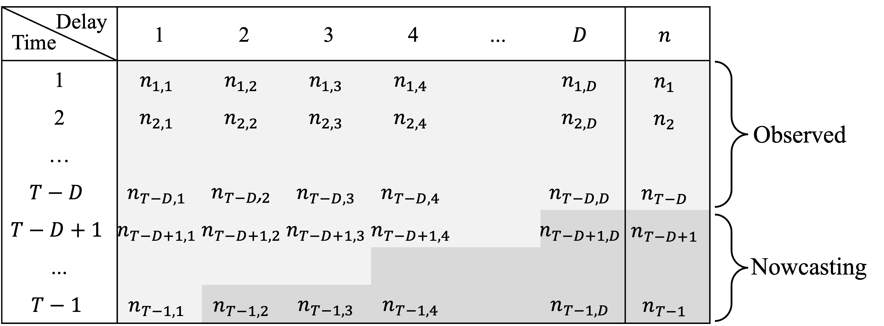
Figure 1 shows the data structure for the reporting delay of cyber incidents based on the breach data. The rows correspond to time $t = 1, 2,\ldots,T$, and $T$ is the present time. The columns correspond to the amount of delay in the same unit as $t$. In our data, the unit is set to be one month. $n_{t,D}$ represents the number of incidents reported between $(D-1)$th and $D$th months after occurrences at time $t$. For example, for the first row, $n_{1,1}$ represents the number of breach incidents that occurred during the first month of our study period and were reported within the month after they occurred, $n_{1,2}$ incidents were reported between the second month after occurrence, and $n_{1,3}$ incidents were reported between the second and third month after occurrence. In our study, we chose $D=12$ because one year is a typical choice for the reserving period (Wüthrich and Merz 2008). That is, incidents with delays longer than one year were excluded from the current study. The last column, $n_t$, represents the total incidents occurring at time period $t$. Since the current time is $T$, the completely observable times are from 1 to $T-D$. From $T-D+1$ to $T-1$, we can observe only partial observations and need to nowcast the incidents (i.e., determine the number of IBNR incidents).

Figure 1.Data structure in the reporting delay of cyber incidents. The values in the gray area represent observed data, and the values in the dark gray area represent the number of IBNR events. Unit: month.

The dataset studied is divided into 72-month time periods. For the purpose of assessing model performance, we use the first 60 months as the in-sample data (i.e., January 1, 2018, to December 31, 2022) and the rest of the data as the out-of-sample data (i.e., January 1, 2023, to December 31, 2023), i.e., $T=61$.

Figure 2.Time series plots and boxplots of frequencies of the number of data breaches reported with different delay periods. The red dot in the boxplot represents the mean and the $x$-axis represents the number of months of delay.

Figure 2, panel (a) illustrates the time series plots of the frequency of the number of data breaches reported with different delay periods for the in-sample data. The number of incidents in different delayed months changes over time, showing an increasing trend in recent months. Particularly, we see a jump in December 2022 (i.e., 155 incidents occurred and were reported in this month). Most of the incidents were delayed in the first three months. Figure 2, panel (b) further shows the boxplots of frequency in various delayed months. It is clear that the frequency shows a decreasing trend over delayed months. This suggests that the time effect needs to be incorporated into the modeling process.

Figure 3.Correlation plots of frequencies in different delayed months, where “m” is the abbreviation for month.

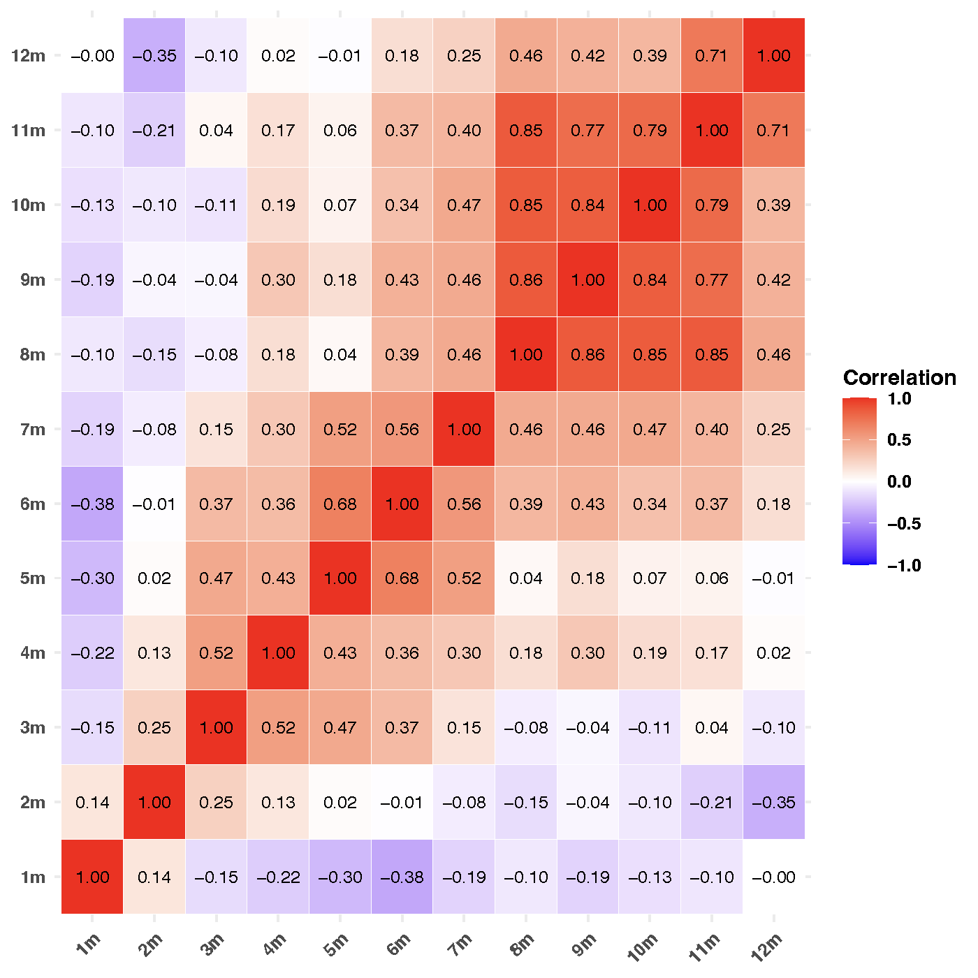
Figure 3 shows the correlation plots of the frequency among different delayed months. We observe correlations among adjacent months. It is interesting to see the high correlations among large adjacent delayed months (e.g., 10/11/12 months), which occur because there are few incidents reported in those large delayed months. This suggests that the correlations among different delayed months should also be considered.

3. Bayesian nowcasting model

The Bayesian nowcasting model proposed in this study aims to capture the time effect and correlations among the delayed months in the number of data breach events that occur but are not yet reported. Define a random variable $n_{t,d}$ that represents the number of events that occur at time $t$ (where $t = 1,2,\ldots,T-1$) but are not reported until time $d$ (where $d = 1,2,\ldots,D$). The model assumes that $n_{t,d}$ follows a negative binomial distribution,

$$n_{t,d} \sim \text{NB}(p_{t,d},r_{t,d}), \tag{1}$$

where $p_{t,d}$ is the probability of breach and $r_{t,d}$ is the number of breaches. The proposed distribution is very flexible as it allows the probability and number of branches to vary with the time and the delayed month. To capture the effect and correlations among the delayed months, we propose the following Bayesian model:

$${\rm logit}(p_{t,d})=\alpha_0+\alpha_1 t+\alpha_2 d/D, \tag{2}$$

and

$$\log(r_{t,d}) = \beta_0+\beta_1 t+\beta_2 d/D, \tag{3}$$

where

$$\alpha_i \sim N\left(0,\sigma^2_{\alpha_i}\right), \quad i = 0,1,2,$$

and

$$\beta_j\sim N\left(0,\sigma^2_{\beta_j} \right), \quad j = 0,1,2.$$

Equation (2) models the breach probability with logistic regression with random effects, and Equation (3) models the log-transformed number of incidents with a regression model with random effects. The prior distributions for the random effects are assumed to be normal distributions. The variability of the random effects is incorporated by assigning prior distributions, a standard exponential distribution, to the parameters $\sigma_{\alpha_i}$ and $\sigma_{\beta_j}$. That is,

$$\sigma_{\alpha_i}\sim {\rm Exp}(1),\quad \sigma_{\beta_j}\sim {\rm Exp}(1),$$

for $i,j =0,1,2$. The posterior distribution for the model parameters $\Theta = (\alpha_i,\beta_j, \sigma_{\alpha_i},\sigma_{\beta_j})$ can be represented as

$$p(\Theta|\mathbf{n}) = p(\Theta) \prod_{t=1}^{T-1} \prod_{d=1}^{D} p(n_{t,d}|\Theta), \tag{4}$$

where $p(\Theta|\mathbf{n})$ follows the negative binomial distribution and $\mathbf{n}$ represents all the observed data. The joint prior distributions $p(\Theta)$ are specified for the model parameters. The estimation of posterior distributions is performed using Markov Chain Monte Carlo (MCMC) methods (Liu 2001; de Valpine et al. 2017).

In our study, the IBNR nowcasting is done by estimating the posterior predictive distribution

$$p(n_{t,d})=\int_{\Theta} p(n_{t,d}|\Theta) p(\Theta|\mathbf{n}) d\Theta,\tag{5}$$

where the MCMC approach is used to obtain samples from the posterior predictive distribution.

In practice, to address scalability concerns, our model can leverage parallel computing methods to enhance efficiency, particularly in handling computationally intensive tasks of MCMC sampling. By running multiple MCMC chains in parallel across different cores, we can significantly reduce the time required for parameter estimation and model convergence. This parallelization allows the model to scale effectively to larger datasets without compromising performance, making it feasible for practical applications in real-world scenarios. For example, the use of parallel processing tools, such as the doParallel package in R (Weston and Calaway 2022), allows us to distribute computational load and maintain manageable runtime even as the dataset expands.

4. Synthetic data study

To understand the model performance, we examine the model performance on a synthetic dataset. The data are generated from a negative binomial distribution with

$${\rm logit}(p_{t,d})=-1.5-.01t+.8d/D,$$

$$\log(r_{t,d})=1.5+.01t-1.8d/D,$$

where $t=1,\ldots, 72$; $d=1,\ldots,12$; and $D=12$.

Figure 4.Time series plots and box plots of frequencies of the number of data breaches reported with different delay periods. The red dot in the boxplot represents the mean and the $x$-axis represents the number of months of delay.

The time series plots of delayed months are displayed in Figure 4, panel (a). We observe that a significant portion of simulated incidents is reported within the initial months following the occurrence. The time series shows variability and an increasing trend in recent months. The box plots in Figure 4, panel (b) reveal that the data are skewed, as indicated by the comparatively large means. Furthermore, there is large variability across the dataset, particularly within the initial months of delay (up to four delayed months). In addition, the presence of outliers within the simulated sample further underscores the heterogeneity of incident-reporting patterns.

Figure 5.Traceplots of parameters in Equation (2).

Figure 6.Traceplots of parameters in Equation (3).

We use the following settings in the model fitting. Three MCMC chains are used to estimate the posterior distributions to ensure convergence and assess the robustness of the results. The initial values are randomly generated based on prior distributions. The burn-in sample is set to be $1e+06$, while the number of iterations is $1.1e+06$. To reduce autocorrelation between samples, we use 100 as the thinning parameter, i.e., every 100th sample will be retained from each chain.

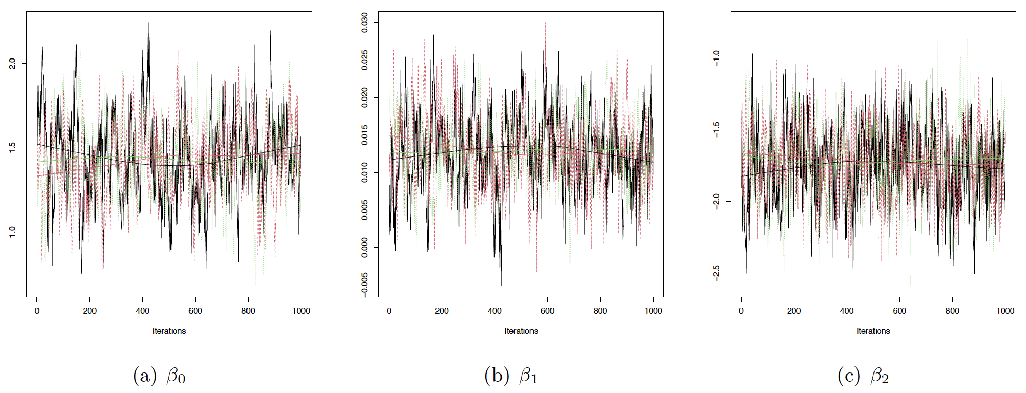
To evaluate the convergence of the Markov chains under consideration, we examine the traceplots for the parameters of Equation (2) presented in Figure 5 and for the parameters of Equation (3) shown in Figure 6. These plots reveal that all three chains demonstrate patterns indicative of convergence. In addition to visually inspecting the traceplots, we quantitatively assess convergence using the Potential Scale Reduction Factor (PSRF). The PSRF compares the variance within each chain to the variance across chains, as proposed by Brooks and Gelman (Gelman and Rubin 1992; Brooks and Gelman 1998). For all the parameters under study, the PSRF values are uniformly less than 1.01, with the multivariate PSRF also recorded at 1.01. These findings provide robust evidence of convergence across the MCMC chains in our analysis, underscoring the reliability of the sampling process in capturing the underlying statistical properties of the model.

Table 1 presents the posterior means and corresponding 95% Bayesian credible intervals for the estimated parameters. We observe that the posterior means demonstrate a close proximity to the true values, indicating a robust performance of the estimation procedure. Furthermore, all 95% Bayesian credible intervals encompass the true parameter values, signifying the reliability and accuracy of the Bayesian inference process.

Figure 7.Nowcast the IBNR cyber incidents.

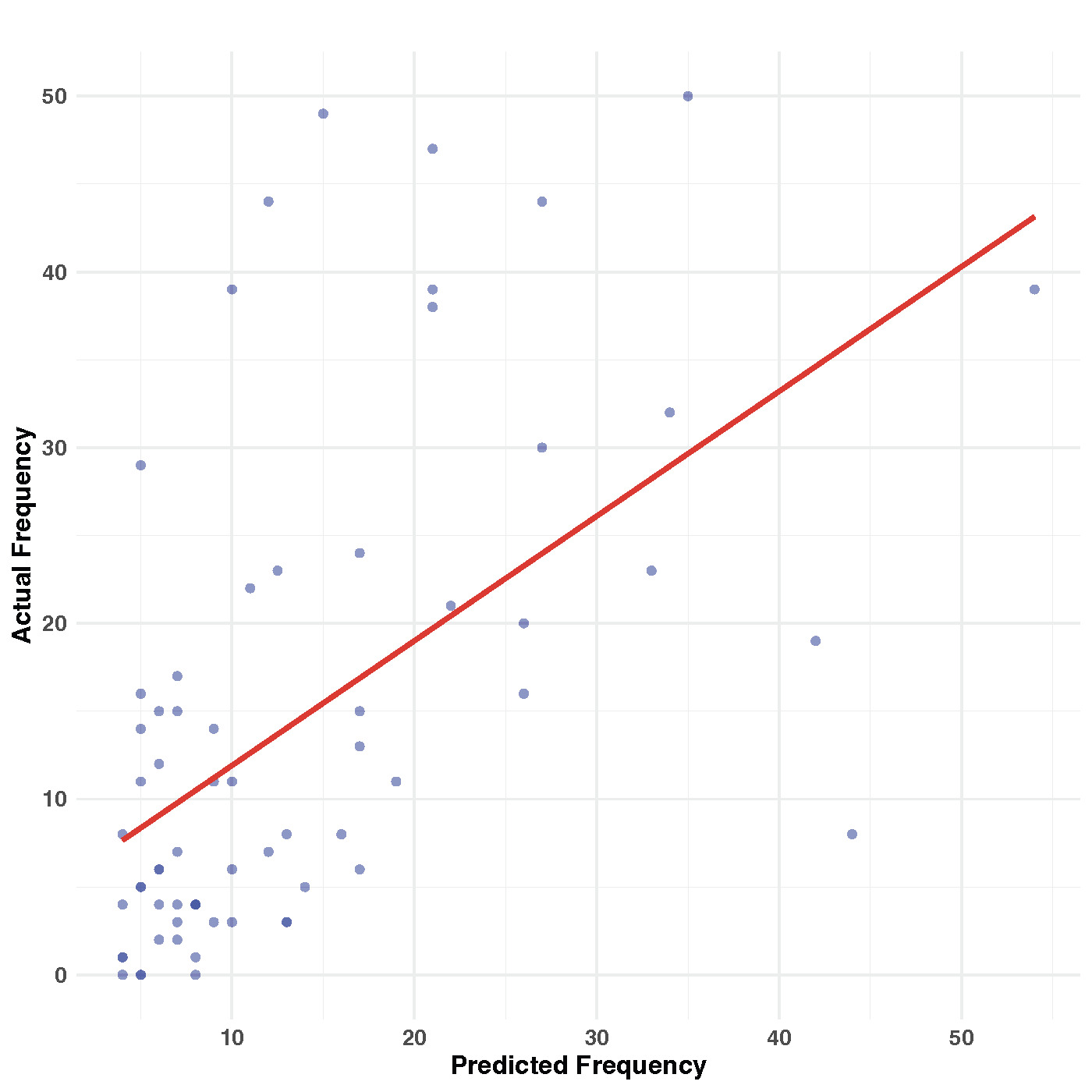
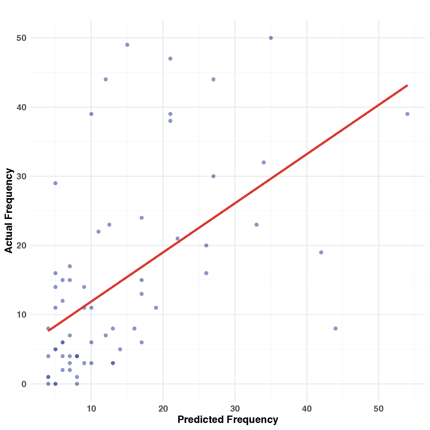
An advantage of using the Bayesian approach is the direct simulation of nowcasts from the model itself. In our analysis, we use the simulated median as the prediction. Figure 7 illustrates a scatter plot comparing the nowcasted frequencies with the real frequencies. Upon inspection, it becomes apparent that there are instances in which the model underpredicts the frequencies. One possible explanation for this discrepancy could be the presence of outliers in the synthetic data, as observed in Figure 4. Despite the presence of outliers, the Pearson correlation coefficient of 0.548 suggests a reasonably strong positive correlation between the nowcasted and real frequencies. This correlation indicates that the proposed model demonstrates good predictive performance when applied to synthetic data, even in the presence of outliers.

Sensitivity analysis. In the following, we perform a sensitivity analysis of the parameter estimates. In the proposed model, prior distributions are specified as standard exponential distributions. We investigate the impact of varying the rate parameter values, specifically using rates of $0.1$, $0.5$, $5.0$, and $10.0$ on the resulting estimates.

The sensitivity analysis, as shown in Table 2, demonstrates how posterior estimates for key parameters respond to variations in the rate parameter for the prior distribution. We observe that the posterior means and 95% credible intervals remain relatively stable, indicating robustness to prior specifications. For example, the parameter $\alpha_0$ consistently shows a posterior mean close to –1.5, with small biases ranging from –0.0467 to –0.0116 across rate values and credible intervals that span similar ranges. The parameters $\alpha_1$ and $\beta_1$ display negligible bias, remaining close to their true values of –0.01 and 0.01, respectively. Some parameters, such as $\alpha_2$ and $\beta_2$, exhibit slightly larger biases, particularly at lower rate values, suggesting sensitivity to the prior distribution’s assumptions. For instance, the bias for $\alpha_2$ ranges from 0.1348 to 0.1955, while $\beta_2$ shows a bias between 0.1166 and 0.1735. These larger biases reflect the influence of the prior on these parameters. However, the credible intervals remain consistent across rate variations, suggesting that the model remains reliable under different prior specifications.

Overall, this analysis indicates that the posterior estimates are largely robust to prior rate changes, with only minor variations in bias for specific parameters.

5. Empirical study

In this section, we apply the proposed model to the ITRC data. Recall that the in-sample data are from January 1, 2018, to December 31, 2022, while the out-of-sample data are from January 1, 2023, to December 31, 2023.

5.1. Model fitting

In our Bayesian model, we use three chains to estimate posterior distributions, initializing them with random values drawn from standard exponential distributions based on prior information. We set the burn-in sample to $2.0 \times 10^6$, with a total number of iterations at $2.1 \times 10^6$. Again, we use a thinning parameter of 100 to ensure efficient sampling.

Examining the traceplots for the parameters depicted in Figure 8 and Figure 9, it is evident that all three chains exhibit patterns suggestive of convergence. These traceplots provide a visual representation of how the parameter values evolve during the sampling process. The convergence patterns observed in the traceplots indicate that the chains have reached stable distributions, suggesting that the MCMC algorithm has successfully explored the posterior space and obtained reliable estimates of the model parameters.

Figure 8.Traceplots of parameters in Equation (2).

Figure 9.Traceplots of parameters in Equation (3).

For all parameters investigated, the PSRF values consistently register at less than 1.01, with the multivariate PSRF also measured at 1.01. These results offer compelling evidence of convergence across the MCMC chains used in our analysis.

Table 3 displays the posterior mean and 95% Bayesian credible intervals for the parameters within our proposed model. The parameter estimates $\alpha_1$ and $\alpha_2$ exhibit varying degrees of influence on the model’s dynamics. Specifically, $\alpha_1$ presents a negative impact, suggesting increased difficulty in system breaches during recent years. In contrast, the positive effect of $\alpha_2$ indicates that, when breaches do occur, their discovery might be delayed, reflecting potentially slower detection processes or more sophisticated breach tactics. Further analysis of the $\beta$ parameters reveals additional insights. $\beta_1$ shows a positive effect, suggesting an increase in the frequency of incidents in recent years. Conversely, $\beta_2$ indicates a negative effect, which could be interpreted as a reduction in the number of incidents with long delays before discovery. While the mean estimate for $\alpha_1$ might initially suggest a minimal impact on the model, its inclusion enhances the model’s predictive accuracy. This highlights the nuanced role $\alpha_1$ plays in the model, potentially capturing dynamics in system breach incidents and their detection timelines. Therefore, despite its seemingly minor direct impact, we include $\alpha_1$ in our analysis.

5.2. Nowcasting performance

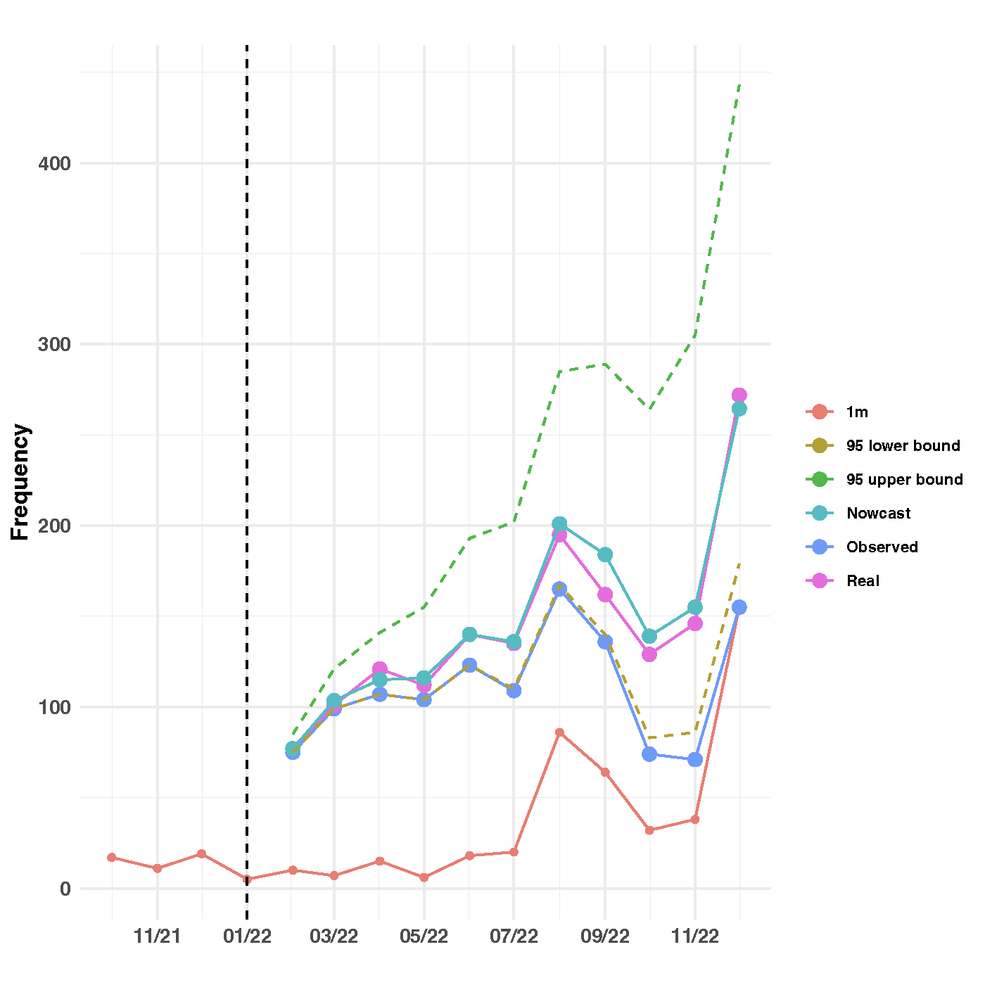
In our model, the median of simulated samples is used as the prediction. Figure 10 presents the nowcasting outcomes accompanied by 95% prediction intervals, juxtaposed with the observed incident counts. The “1m” line reveals a scant number of incidents reported during the respective occurring months. The observed incidents for any given month reflect the cumulative count of occurrences discovered until the end of December 2022. For example, in January 2022, five incidents were reported, while February 2022 saw 18 reported incidents, all of which had transpired in January 2022. Thus, the total number of incidents occurring in January 2022 and reported by the end of December 2022 amounted to 91. Similarly, February 2022 saw 10 reported incidents, yet the total observed incidents for that month by the end of December 2022 stood at 75. The “nowcast” line delineates the total incidents occurring in a specific month and reported within 12 months. For instance, the total number of incidents occurring in February 2022 and reported within 12 months, as estimated by the proposed model, was 77. Conversely, the “real” line portrays the total incidents occurring in a specific month and observed within 12 months, based on testing data. In the case of February 2022, the total observed incidents by the end of January 2023 amounted to 77. Figure 10 illustrates a close alignment between the nowcast and real incident counts during the initial months, with slight deviations in subsequent months. This discrepancy can be attributed to the reduced number of observations in later months, which is evident from the wider prediction intervals.

Figure 10.Nowcast the IBNR cyber incidents. The “1m” line represents the number of cyber incidents that are reported during the occurring month. The dashed “95 lower bound” and “95 upper bound” lines represent the 95% prediction bounds based on the proposed model. The observed number of incidents represents all the incidents that were observed until December 2022.

Figure 11.Nowcast the IBNR cyber incidents.

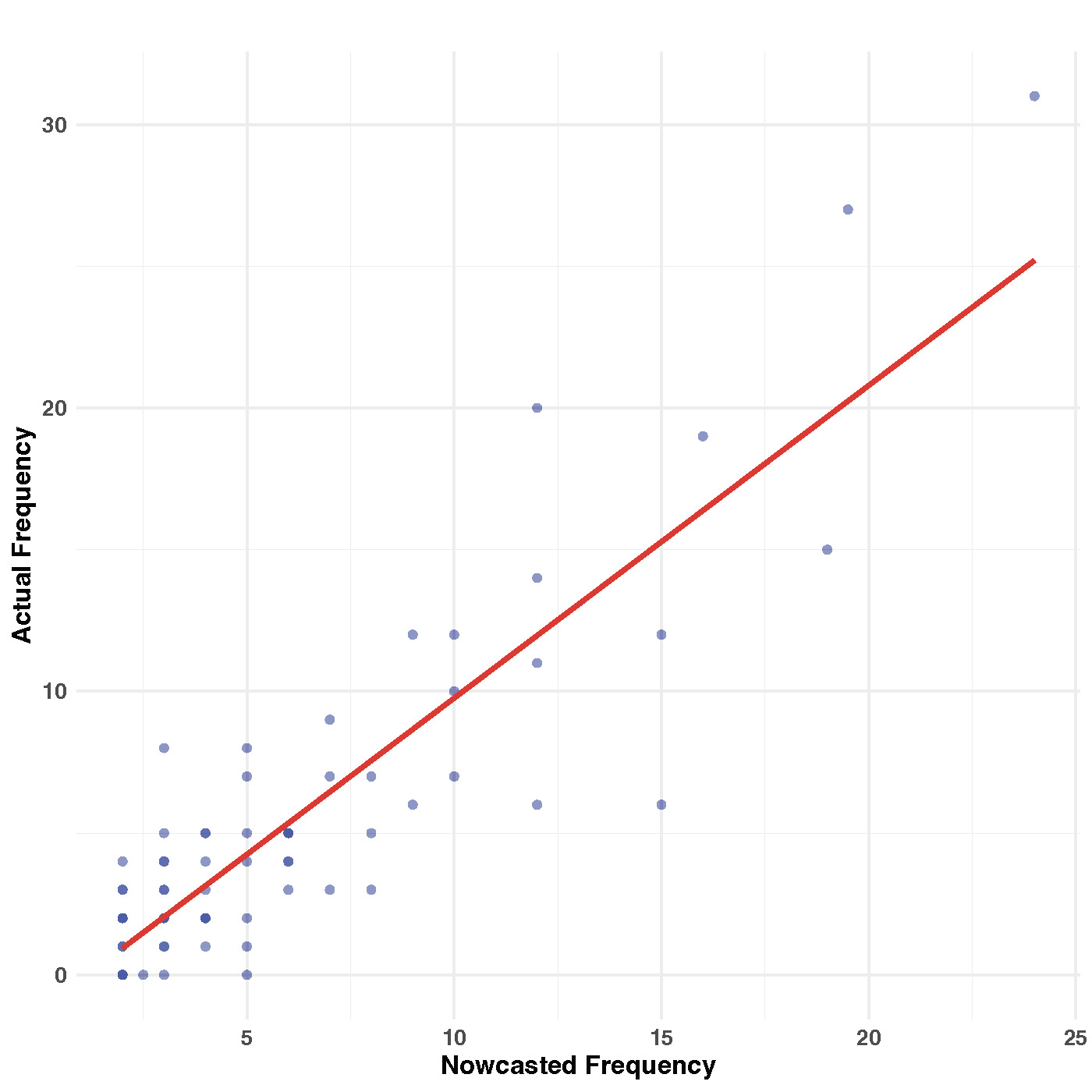
Similarly, we apply the Bayesian approach to nowcast the delayed incidents, utilizing the simulated median as the prediction. Figure 11 presents a scatter plot comparing the nowcasted frequencies with the real frequencies. Remarkably, a high correlation between the two is evident, with the Pearson correlation coefficients reaching 0.875. This substantial correlation suggests that the proposed model demonstrates robust predictive performance.

Model comparison. To further assess the model’s performance, we compare the proposed model (labeled M0) with other ones commonly used in the literature.

• M1: The chain-ladder model (Barnett and Zehnwirth 2000) is the most commonly used approach in practice. It assumes that the proportional developments of claims from one development period to the next are the same for all origin periods.

• M2: The Mack chain-ladder model (Mack 1993, 1999) is a distribution-free stochastic model underlying the chain-ladder approach. Let $S_{ik}$ denote the cumulative claims of origin period (e.g., accident year) $i=1,\ldots,m$, with claims known for development period (e.g., development year) $1\leq k\leq n+1-i$. To forecast the amounts $S_{ik}$ for $n+1-i< k\leq n$, the Mack chain-ladder model assumes

  $$\begin{aligned} &{\rm E}[F_{i,k}|S_{i1},S_{i2},\ldots S_{ik}]=f_k~{\rm with}~F_{i,k}=\frac{S_{i,k+1}}{S_{ik}},\\ &{\rm Var}[F_{i,k}|S_{i1},S_{i2},\ldots S_{ik}]=\frac{\sigma_{k}^2}{w_{ik}S_{ik}^\alpha},\\ &(S_{i1},S_{i2},\ldots S_{in}) ~\mbox{are independent by}~i,~1\leq i\leq n\textit{,} \end{aligned}$$

  with $w_{ik}\leq [0,1]$, $\alpha\in \{0,1,2\}$.

• M3: The bootstrap chain-ladder model (England and Verrall 1999) uses a two-stage bootstrapping methodology to forecast the trajectory of the development runoff. In the initial stage, the model applies the ordinary chain-ladder method to the cumulative claims triangle. Subsequently, scaled Pearson residuals are computed from this stage, and through bootstrapping iterations ($R=1,000$ times in our study), future incremental claims payments are projected using the standard chain-ladder method. Moving to the second stage, the process error is simulated by incorporating the bootstrapped values as means while adhering to the assumed process distribution. The resulting set of reserves derived from this approach constitutes the predictive distribution. For the bootstrap chain-ladder model, we use the median as the prediction.

• M4: In the generalized linear model, Renshaw and Verrall (1998) proposed a methodology for modeling incremental claims using an overdispersed Poisson distribution. If we denote the incremental claims for origin year $i$ in development year $k$ as $C_{ik}$, the model is characterized by the following equations:

  $$\mathbb{E}[C_{ik}] = m_{ik}\textit{,} \quad \text{and} \quad \text{Var}[C_{ik}] = \phi \mathbb{E}[C_{ik}] = \phi m_{ik}\textit{,}$$

  where $\phi$ is a scale parameter, $\log(m_{ik}) = \eta_{ik}$, and $\eta_{ik}= c + \alpha_i + \beta_k$, with $\alpha_1= \beta_1 = 0$. It is a generalized linear model wherein the response is modeled using a logarithmic link function and the variance is directly proportional to the mean.

• M5: Random Forest (Breiman 2001) is a popular machine learning model based on an ensemble of decision trees; it can capture nonlinear patterns in data. Since our data are not typical regression data as they do not include features/covariates, we generated lagged features that represent previous values in each row as predictors for the target variable. We perform the predictions based on steps taken prior to time. We applied mean imputation, replacing each missing feature with the mean of the respective column calculated from the observed data.

• M6: XGBoost (Chen and Guestrin 2016) is another advanced machine learning model; it uses gradient boosting with optimized tree structures to minimize error. For data preparation, we generated lagged features in the same manner as we did with Random Forest. However, XGBoost can handle missing values directly using a sparsity-aware algorithm. It determines the optimal direction in which to assign instances with missing values during tree construction. Thus, we directly provided XGBoost with lagged features containing missing values (written as NA), allowing the algorithm to account for missingness patterns as potential predictors.

Model comparison based on root-mean-square error (RMSE) and mean absolute error (MAE) is a common approach to assessing the predictive performance of different models. RMSE measures the average squared difference between predicted values and actual values, while MAE measures the average absolute difference between predicted values and actual values.

Table 4 displays the prediction results from various models; it is evident that the performance of the models varies significantly. The proposed model M0 exhibits the lowest RMSE and MAE, indicating superior predictive accuracy compared to the other models. Conversely, Model M1 demonstrates the highest RMSE and MAE values, suggesting poorer predictive performance. Models M2 and M3 have intermediate RMSE and MAE values, while Model M4 has a relatively poor prediction performance. The machine learning models, M5 and M6, show improvement over traditional models such as M1 but fall short of the accuracy demonstrated by M0, with RMSE values of 17.3243 and 19.3444, respectively. Although machine learning approaches have proven highly effective in many predictive contexts, they do not achieve satisfactory performance in our setting. This is primarily due to the absence of informative features or covariates relevant to the nowcasting task.

In summary, the proposed model demonstrates satisfactory nowcasting performance, effectively estimating incident counts with high accuracy.

5.3. Reserve estimation

We apply the results derived from our proposed Bayesian model to estimate the financial impact of cyber incidents, leveraging the average cost of a data breach. According to IBM’s 2022 report,^[4] the average cost of a data breach incident is estimated at $4,350,000. This value serves as the per-incident cost in our analysis. By integrating this cost metric with the model’s nowcast incident frequency, we can approximate the total financial impact and the insurance reserves that are expected to cover during the year.

Table 5 presents the reserve estimation for cyber incidents in 2022, using the proposed Bayesian model. We calculate monthly figures for estimated, paid, IBNR, and ultimate claims, all denominated in millions based on the nowcast frequencies, wherein the ultimate claims are computed by using the out-of-sample data of 2023. A consistent trend observed during the year is the widening discrepancy between estimated and paid claims, leading to a significant accumulation of IBNR claims. The peak in estimated claims was witnessed in December, surging to 1,150,575,000, alongside a notable increase in IBNR claims to 476,325,000. It is interesting to see that the IBNR rate shows an overall decreasing trend. The comparative analysis of estimated versus ultimate claims underscores the good performance of the proposed Bayesian model in managing the uncertainties in cyber incident claims. With estimated total claims reaching 7,490,700,000, slightly above the ultimate claims of 7,312,350,000, the model exhibits a marginally conservative bias. Nevertheless, this nuance further underscores the model’s significant promise in refining actuarial methodologies for cyber risk management.

6. Conclusion and discussion

This work introduces a novel Bayesian nowcasting model tailored to estimate IBNR cyber incidents. Through synthetic and empirical data studies, the model demonstrates exceptional predictive accuracy, outperforming traditional models commonly used in actuarial science, such as the chain-ladder and generalized linear models. The application of our model in reserve estimation, using the average cost of a data breach reported by IBM, offers a refined approach to quantifying the financial implications of cyber incidents. This not only provides reserves estimations but also contributes valuable insights into the dynamic nature of cyber risk exposure. The proposed Bayesian nowcasting model represents a significant advancement in actuarial science, particularly in the domain of cyber risk management. Its ability to effectively integrate temporal and correlation effects among delayed reporting intervals sets a new benchmark for predictive analytics in insurance reserves.

We acknowledge the ethical implications of using data breach information for modeling purposes, as such incidents often involve sensitive or personal information. For this study, only publicly available and aggregated data sources are used, ensuring that no personal identifiers or details compromising individual privacy are included. The model’s primary aim is to enhance understanding of breach reporting patterns to support risk mitigation and preparedness for insurers. In addition, all utilized real-world data comply with applicable privacy regulations (e.g., data breach notification requirements under federal laws and state legislation) to uphold the confidentiality of affected parties.

While this study focuses on cyber incidents, the proposed model is adaptable to other types of insurance claims for which reporting delays are a concern. By integrating more detailed data regarding the specifics of cyber incidents, the model’s predictive capabilities can be enhanced. For instance, in the context of reserve estimation, using actual cost data for each incident, rather than relying on average costs, would likely yield more precise outcomes. Nonetheless, obtaining such detailed cost data is often challenging in practice, presenting a notable limitation to this approach. Furthermore, exploring a joint modeling approach that simultaneously considers both the frequency of incidents and their associated costs promises to refine the model’s performance even further. Applying this model to real-world scenarios hinges on the availability and quality of empirical data to ensure accurate and reliable results. However, real-world cyber incident data often face challenges such as underreporting, delays in disclosure, and inconsistencies across industries and organizations. These limitations can introduce biases that may affect the model’s nowcasting accuracy. One approach to mitigating these issues is to focus on severe incidents that result in substantial financial losses, as these are often subject to mandatory reporting within specific time frames following detection. This focus can help reduce bias and improve the reliability of the model’s predictions.

Acknowledgments

The authors are grateful to the anonymous referee for the insightful and constructive comments, which led to this improved version of the article. Any opinions, findings, conclusions, or recommendations expressed in this material are those of the authors and do not necessarily reflect the views of the CAS.