Statistical Modeling of Data Breach Risks: Time to Identification and Notification

1. Introduction and motivation

A data breach poses devastating risks to computer systems. Data breaches are a growing problem that is likely to worsen, given the rapid expansion of what are already enormous network activities. Many severe cybersecurity incidents have occurred in recent years. For example, the Privacy Rights Clearinghouse reported that more than 11 billion records have been breached since 2005.^[1] The Identity Theft Resource Center and Cyber Scout reported 1,108 data breach incidents in 2020, affecting 310,116,907 individuals; the number of incidents increased to 1,862 in 2021, affecting 293,927,708 individuals.^[2] Each data breach incurs substantial costs. According to IBM’s Cost of a Data Breach Report 2021,^[3] the average cost of a data breach incident increased from $3.86 million in 2020 to $4.24 million in 2021, and the average per-record cost of a data breach increased 10.3% between 2020 and 2021, from $146 to $161.

Given the unique nature of cyber risk, the discovery of a breach is often delayed by several days, months, or even years after the initial breach. The longer a breach remains undetected, the more data are exposed, amplifying both the financial and broader consequences. For example, according to the 2021 IBM report, the mean times to data breach discovery for 2019, 2020, and 2021 were 206, 207, and 212 days, respectively; the mean times to data breach containment (i.e., the mean length of a breach life cycle) for those years were 279, 280, and 287 days, respectively. The report also pointed out that the faster a data breach can be identified and contained, the lower the cost. For example, in 2021 a breach with a life cycle of more than 200 days cost an average of $4.87 million, compared with $3.61 million for a breach with a life cycle of fewer than 200 days. This finding is consistent with the simulation study of Hua and Xu (2020), which found that reducing the time to identification is the key to reducing costs. The time to notification is another important factor contributing to data breach costs. Notification allows affected individuals to take proactive steps (e.g., changing passwords, monitoring credit scores, etc.), thereby reducing the number of potential lawsuits against the organization. However, to our knowledge, no formal statistical approach exists yet for modeling time to identification (TTI) and time to notification (TTN), with only one relevant work, Bisogni, Asghari, and Van Eeten (2016), where the authors used negative binomial regression to study the relationship between TTI and other factors.

Since data breaches have become the most common and dangerous cyber risk we face today, researchers have begun to investigate the development of statistical models to analyze data breaches. Some of these studies are loosely related to our current study. For example, Romanosky, Telang, and Acquisti (2011) used a fixed effect model to estimate the impact of data breach disclosure policy on the frequency of identity thefts following data breaches. Buckman et al. (2017) studied the time intervals between data breaches for enterprises that had at least two incidents between 2010 and 2016 and found that the duration between two data breaches may increase or decrease, depending on certain factors. Edwards, Hofmeyr, and Forrest (2016) analyzed temporal trends of data breach size and frequency and showed that breach size follows a log-normal distribution and the frequency follows a negative binomial distribution. They further showed that the frequency of large breaches (over 500,000 breached records) follows a Poisson distribution, rather than a negative binomial distribution, and that the size of large breaches still follows a log-normal distribution. Eling and Loperfido (2017) studied data breaches from the perspective of actuarial modeling and pricing, using multidimensional scaling and goodness-of-fit tests to analyze the distribution of data breaches. They showed that different types of data breach should be analyzed separately and that breach sizes can be modeled by a skew-normal distribution. Sun, Xu, and Zhao (2021) developed a frequency-severity actuarial model of aggregated enterprise-level breach data to promote ratemaking and underwriting in insurance. Ikegami and Kikuchi (2020) studied a breach dataset in Japan and developed a probabilistic model to estimate the risk of data breach. The authors found that the inter-arrival times of data breaches for enterprises with multiple breaches followed a negative binomial distribution. Xu and Zhang (2021) showed that a non-stationary extreme value model successfully captures the statistical pattern of the monthly maximum data breach size. They also discovered a positive time trend based on the Privacy Rights Clearinghouse dataset. Using the same dataset, Jung (2021) compared the estimates of extreme value distributions before and after 2014 and reported a significant increase with a break in the loss severity. Recent reviews on cyber risk modeling are also relevant (e.g., Eling (2020); Zeller and Scherer (2022); Woods and Böhme (2021)).

The current study differs from the existing literature in that we studied the statistical properties of TTI and TTN. Our study’s contributions include: (1) We introduced a novel copula approach to tackle the missing data issues because TTN and TTI data are frequently missing, especially TTI data. Compared with commonly used missing data imputation methods, such as Kalman smoothing and multivariate imputation by chained equations (MICE) imputations, our proposed copula approach is simple, efficient and shows better predictive performance. (2) We developed a dependence model to capture the positive dependence between TTN and TTI. Our study showed that the proposed model is superior to other commonly used multivariate time series models. (3) Our model has practical implications that we discuss in this paper.

The rest of the paper is organized as follows. Section 2 covers the exploratory data analysis of the breach data that we conducted to motivate the proposed model. Section 3 introduces preliminary factors for statistical modeling. Section 4 introduces the copula approach for imputing missing data. Section 5 develops the dependence model for TTN and TTI and assesses model performance. Section 6 presents conclusions and offers discussion.

2. Exploratory data analysis

The breach notification data were collected manually from the California Attorney General website,^[4] which provides a list of breach notification reports that include organization name, date(s) of breach (if known), reported date, and a brief description of incident(s). The earliest report is from January 20, 2012, so we studied data from that date through December 31, 2020, for a total of 2,123 breach reports. We organized the data by the date of notification. For example, consider a breach that occurred on January 1, 2020, was discovered on June 1, 2020, and notified on August 1, 2020. In this case, August 1, 2020, is used as the date associated with this observation, and the corresponding TTI and TTN are 152 and 213 days, respectively. For notifications with multiple breach dates for the same incident, we used the earliest breach date in our analysis. For instance, Steel Partners Holdings L.P. submitted a breach notification on November 23, 2020, with two breach dates, April 18, 2020, and April 29, 2020. We used April 18, 2020, as the breach date since both breaches referred to the same incident. The other quantity of interest is the time from identification to notification (ITN), which is the difference between TTN and TTI.

The summary statistics of TTN are reported in Table 1, which shows that the minimum TTN was zero, meaning that a breach was reported the same day it occurred. However, the percentage in this category was small at only $0.09\%$. The mean TTN was 189.8 days (SD $268.29$ days), with a median of $102$ days. Figure 1(a) shows the TTN time series plot, which shows large TTN values, indicating high variability. The box plot in Figure 2(a) shows that TTN is skewed with high variability. The largest TTN, 3,222 days, corresponds to the Dominion National incident reported on June 21, 2019, but the breach occurred as early as 2010,^[5] and was the second-largest breach reported to the Department of Health and Human Services. This incident affected 2.9 million patients and resulted in Dominion National paying out a $2 million settlement. Over the study period, $11.35\%$ incidents had missing data (i.e., unknown breach dates).

Figure 1.TTI and TTN time series plots. Unit: days.

The TTI time series plot in Figure 1(b) shows both large and small values, indicating high variability in TTI. Table 1 shows $18.23\%$ 0s, indicating that only a small percentage of incidents were detected on the same day they occurred. The mean TTI was 101.8 days, but the median was much smaller at 20 days. This suggests that TTI is very skewed, as shown in Figure 2(b). The percentage of missing data was high at $36.65\%$, where either the breach date or the identification date were missing from the breach report. The maximum TTN was 3,140 days and it corresponds to the same incident that had the maximum TTN of 3,222.

Table 1 shows that the mean ITN was 62.01 days (SD 60.92 days), with a median of 44 days. California data breach laws require notification to be as expedient as possible, without unreasonable delay.^[6] It should be noted that data breach laws are enacted at the state level, and notification requirements across states range from 24 hours to 90 days.^[7] The box plot in Figure 2(c) shows many large TTN values greater than 90 days.

The maximum ITN was 539 days, which corresponds to the UC San Diego Health incident reported on June 14, 2019. In this incident, HIV research participants’ sensitive data were made accessible to employees of Christie’s Place, a San Diego nonprofit that supports women with HIV and AIDS. The organization was criticized for the delay in notifying women affected by the breach.^[8]

Figure 2.TTN, TTI, and ITN box plots. Unit: days.

Yearly TTN and TTI statistics are also of interest; summary statistics are shown in Table 2. TTN means in the first two years were smaller than those in the other years, with the mean ranging from 122 days in 2012 to 223.19 days in 2017. TTN standard deviations were large for all years. The median TTN shows an overall increasing trend, which is further confirmed by the TTN box plot in Figure 3(a), which shows high variability. The TTN box plot also indicates that the TTN distribution is heavily skewed.

Figure 3.Yearly TTN and TTI box plots

The TTI means and medians do not show any clear patterns. Each year had more 0s compared with that of TTN. TTI also showed high variability and the medians were much smaller than the means. The TTI box plot in Figure 3(b) also shows that the TTI distribution is heavily skewed.

To summarize, both TTN and TTI had substantial missing data; the percentage of missing dates in TTI was over 36%. Both TTN and TTI are heavily skewed and showed high variability, indicating that the mean is an unreliable TTN/TTI risk measure. We took this finding into account in our modeling process.

3. Preliminaries

This section introduces preliminaries pertinent to the following discussion.

3.1. Copula

Copula is an effective tool to model high-dimensional dependence and has been widely used in many areas (Joe 2014). Let $X_1,\ldots,X_d$ be continuous random variables with univariate marginal distributions $F_1,\ldots,F_d$, respectively. Denote their joint cumulative distribution function (CDF) by

$$F(x_1,\ldots,x_d)=P(X_1\le x_1,\ldots,X_d\le x_d).$$

A $d$-dimensional copula, denoted by $C$, is a CDF with uniform marginals in $[0,1]$, the joint CDF of the random vector $(F_1(X_1),\ldots,F_d(X_d))$. Sklar’s theorem (Joe 2014) states that when the $F_i$’s are continuous, $C$ is unique and satisfies

$$F(x_1,\ldots,x_d)=C(F_1(x_1),\ldots,F_d(x_d)).$$

Let $c(u_1,\ldots,u_n)$ be the $d$-dimensional copula density function and $f_i$ be the marginal density function of $X_i$ for $i=1,\ldots, d$. The joint density function of $(X_1,\ldots, X_d)$ is

$$f(x_1,\ldots,x_d)=c(F_1(x_1),\ldots,F_d(x_d))\prod_{i=1}^d f_i(x_i).$$

We used a bivariate copula to model the dependence between TTN and TTI specifically considering the Tawn type II copula and a BB8 copula. Appendix A provides more details on these copulas (Joe 2014).

3.2. ARMA, GARCH, DCC, and VAR models

Autoregressive moving average (ARMA) and generalized autoregressive conditional heteroskedasticity (GARCH) are widely used time series models (Cryer and Chan 2008). The ARMA($p$,$q$) model has the general form:

$$X_t = \mu + \sum_{k=1}^{p} \phi_k X_{t-k} + \sum_{l=1}^{q}\theta_l\epsilon_{t-l} + \epsilon_t$$

where $\phi_k$, $\theta_{l}$ are the parameters of AR and MA, $\mu$ is the intercept, and $\epsilon_{t}$ is the innovation of the time series. For the GARCH$(p,q)$ model, this can be rewritten as $X_t=\sigma_t \epsilon_t$, and

$$\sigma_t^2=w+\sum_{j=1}^q \alpha_j \epsilon_{t-j}^2+\sum_{j=1}^p \beta_j\sigma^2_{t-j},$$

where $\alpha_j$ and $\beta_j$ are the coefficients, $\sigma_t^2$ is the conditional variance, and $w$ is the intercept.

The dynamic conditional correlation (DCC) model introduced by R. Engle (2002) provides a good approximation for many time-varying correlation processes. Let ${\bf x}_t = (x_{1,t},x_{2,t},...,x_{m,t}$) be a vector for $m$-dimensional time series at time $t$. A multivariate GARCH model is defined as

$${\mathbf{x}}_t = H_t^{1/2}{\boldsymbol{\epsilon}}_t$$

where $H_t$ is an $m\times m$ conditional covariance matrix, and ${\boldsymbol{\epsilon}}_t$ is an $m\times 1$ vector of error with mean and variance given by $E({\boldsymbol{\epsilon}}_t) = {\mathbf{0}}$ and ${\rm{Var}}({\boldsymbol{\epsilon}}_t) = I_m$ where $I_m$ is an $m\times m$ identity matrix. The covariance matrix $H_t$ can be decomposed into

$$H_t = D_tR_tD_t$$

where $D_t$ = ${\rm diag}({\sqrt{h_{11,t}},...,\sqrt{h_{mm,t}}} )$ is a diagonal of time-varying standard deviations from a univariate GARCH$(p,q)$ model, and $R_t$ is a time-varying positive definite conditional correlation matrix

$$R_t = {\rm{diag}}(Q_t)^{-1/2}Q_t{\rm{diag}}(Q_t)^{-1/2}$$

where

$$Q_t = (1-a-b)\bar{Q} + a{\mathbf{z}}_{t-1}{\mathbf{z}}'_{t-1} + bQ_{t-1}$$

is a positive symmetric matrix, and $\bar{Q}$ is the unconditional matrix of the standardized errors ${\bf z}_t = D_t^{-1}{\bf\epsilon}_t$. The condition of $a + b <1$ is imposed to ensure the stationarity and positive definiteness of $Q_t$. The DCC model has two steps: (1) estimate the univariate GARCH parameters, and (2) estimate the conditional correlation $R_t$. See R. Engle (2002) for more details on the DCC model.

Vector autoregressive (VAR) models are commonly used to investigate dynamic interactions in multivariate time series (Tsay 2005). A VAR($p$) model is represented as

$${\bf x}_t = A_1{\bf x}_{t-1} + ... + A_p{\bf x}_{t-p} + {\bf \gamma}_t$$

where $A_i$ is an $m\times m$ coefficient matrix for $i = 1,2,..,p$ and ${\bf\gamma}_t$ is an $m$-dimensional error process with zero mean and a time-invariant positive definite covariance matrix.

3.3. Accuracy metrics

We used the following two metrics to evaluate the predictive distribution accuracy: (1) The commonly used mean absolute error (MAE), which is represented as

$$\mbox{MAE}=\frac{1}{m}\sum_{i=1}^{m} |y_{i}-\hat{y}_{i}|,$$

where $y_{i}$ represents the observed values and $\hat{y}_{i}$ represents the predicted values, $i=1,\ldots,m$. (2) The continuous ranked probability score (CRPS), which is defined as

$$\mbox{CRPS}(F,s)=\int_{\mathbf{R}}(F(y)-\mathbf{1}\{s\le y\})^2dy,$$

where $F(\cdot)$ denotes the CDF and $\mathbf{1}\{\cdot\}$ denotes the indicator function. The CRPS measures the difference between the predicted and empirical CDFs of observed values and is a widely used accuracy measure for probability forecasts (Epstein 1969). A lower score indicates a better prediction.

4. Copula approach to missing data imputation

Let $x_{1,t}$s and $x_{2,t}$s be the observed time series values of TTN and TTI, respectively, $t=1,\ldots,T$. For modeling purposes, we used the January 20, 2012 to December 31, 2018 period as the in-sample data (i.e., 1,505 pairs of observations with 596 NAs) and used the January 01, 2019 to December 31, 2020 period as the out-of-sample data (i.e., 618 pairs of observations with 282 NAs). Since both TTN and TTI contain missing values, we used $x^*_{1,t}$s and $x^*_{2,t}$s to represent the missing TTN and TTI observations, respectively. We proposed a copula approach to imputing the missing data in Algorithm 1 for the in-sample data. The procedure to impute the missing data for TTN and TTI was as follows.

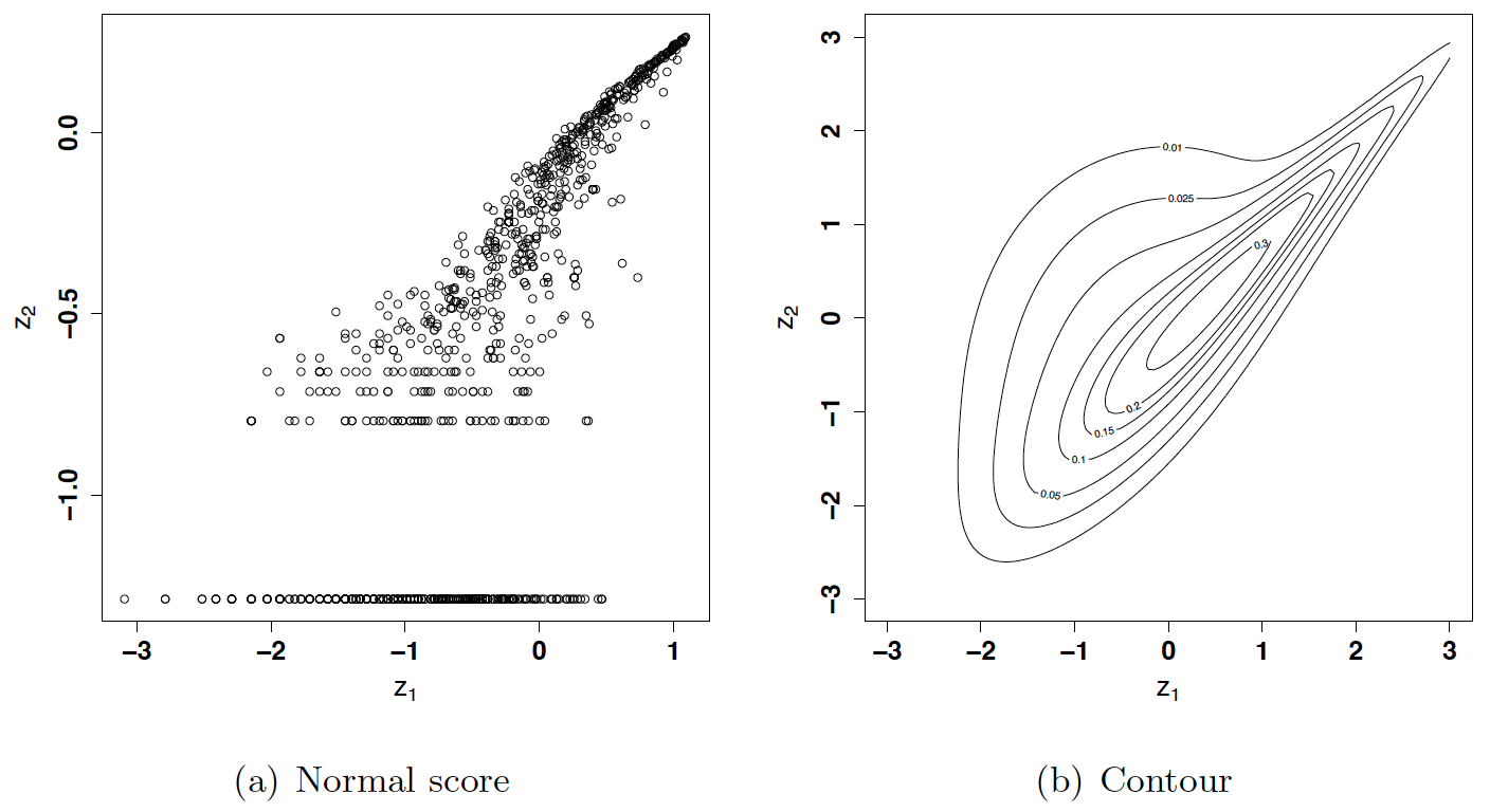
• Model the dependence based on the complete pairs of TTNs and TTIs. Our study had 910 completely observed pairs of TTNs and TTIs for the in-sample data. Empirical marginals were used to model the dependence between TTN and TTI. We selected the best copula structure from various bivariate copula families in the VineCopula package using the AIC criterion (Schepsmeier et al. 2015). A Tawn type 2 copula was selected for modeling the joint dependence; the estimated parameters were $\theta=3.93$, $\delta=0.67$, and $\tau=0.54$. Figure 4 displays the normal score plot and the fitted contour plot, which shows a strong right tail dependence between TTN and TTI. This is consistent with the findings that a longer TTI relates to a longer TTN.

Figure 4.TTI and TTN normal score plot and contour plot. Unit: days.

• Impute missing data for both TTNs and TTIs. TTN and TTI had 203 completely missing pairs because of unknown breach dates. Based on the estimated copula structure and empirical distributions, we simulated $N=5000$ observations using Algorithm 1, where the symbol $\mathstrut^*$ represents the missing value. Missing values were imputed using the means of simulated observations.

• Impute missing data for TTIs with observed TTNs. Since 392 records had only TTNs because identification dates were not reported, we imputed the missing TTIs using a conditional copula approach, i.e., sampling from the conditional Tawn type 2 copula with given TTNs (line 9 in Algorithm 1).

Algorithm 1.Copula approach for imputing missing data

For comparison, we also applied the following two common approaches for imputation of missing data.

• Kalman smoothing (KS) imputation. KS imputation is commonly used and often yields strong performance (Grewal and Andrews (2014); Moritz and Bartz-Beielstein (2017); Huyghues-Beaufond et al. (2020)). We imputed the missing TTN and TTI values on the training data by using KS imputation. Since TTI must not be larger than TTN, we replaced TTI with TTN if the imputed TTI was larger than TTN (130 imputed observations).

• MICE imputation. Next, we applied MICE imputation to the missing values. The MICE method is a principal method for handling missing values (Van Buuren and Groothuis-Oudshoorn 2011). Similar to the KS method, we imputed the missing values using MICE on the training data. We also replaced TTI with TTN when the imputed value of TTI was greater than that of TTN (8 imputed observations).

Table 3 shows the summary statistics of imputed TTNs and TTIs for the proposed copula, KS, and MICE approaches. The TTN means are very close across the different approaches, but the medians differ. The MICE imputation had the smallest median (87), and the copula approach had the largest (113). The standard deviation was the smallest in the copula approach (251.32) and the largest in the MICE approach (262.14). Mean TTI differed, with the smallest (89.46) from the KS imputation and the largest (123.5) from the MICE imputation. The MICE approach had the smallest median (32), and the KS approach had the largest (51). The KS standard deviation was smallest (171.53) and the MICE was largest (236.39). It is interesting to note that the copula approach produced the smallest $Q_3$s for both TTN and TTI. Compared with the KS and MICE imputation approaches, the proposed copula approach was simple and efficient. We also noted that, using the copula approach, all imputed TTNs were no less than the corresponding TTIs.

Since both TTNs and TTIs were skewed and had high variability, we performed transformations. TTN had only two 0s by the copula imputation, so we replaced the 0s with two random values from a uniform $(0,1)$ distribution and performed a log transformation. TTI had a large portion of 0s, so we performed a square root transformation to reduce the variability.

5. Statistical modeling

We developed a copula approach to jointly model the dynamics of TTN and TTI. After imputing the missing values, both transformed TTN and TTI exhibited temporal correlations, as shown by their partial autocorrelation functions (PACFs) in Figure 5.

Figure 5.Transformed TTI and TTN PACFs. Unit: days.

The following section covers capturing the temporal and cross-sectional dependence of TTN and TTI.

5.1. Model fitting

Section 2 showed that both TTN and TTI had high variability. Therefore, we used a GARCH model to identify TTN and TTI volatility. The residual analysis suggested that GARCH$(1,1)$ is sufficient to describe residual volatility for both series. This is consistent with other research findings that higher-order GARCH models are not necessarily better than GARCH$(1,1)$ (Hansen and Lunde 2005). Therefore, we used GARCH$(1,1)$. We used the ARMA$(p,q)$ process to model TTN and TTI means evolution, which led to the following ARMA$(p,q)$+GARCH(1,1) model

$$X_{t}= \mu+\sum_{k=1}^p \phi_{k} X_{t-k} +\sum_{l=1}^q \theta_{l} \epsilon_{t-l} +\epsilon_{t},\tag{1}$$

where $\epsilon_{t}=\sigma_{t} Z_{t}$ with $Z_{t}$ being the i.i.d. innovations, and the $\phi_k$’s and the $\theta_l$’s are the coefficients of the AR and MA parts, respectively. For the standard GARCH$(1,1)$ model, we have

$$\sigma_{t}^2=w+ \alpha_{1} \epsilon^2_{t-1}+ \beta_{1} \sigma^2_{t-1},\tag{2}$$

where $\sigma^2_{t}$ is the conditional variance and $w$ is the intercept. We used the AIC criterion for model selection to determine the orders of the ARMA models. Note that if ARMA$(p,q)$+GARCH successfully accommodated the serial correlations in the conditional mean and conditional variance, no autocorrelation would remain in the standardized and squared standardized residuals. When the AIC criterion suggested selecting multiple models with similar AIC values, we selected the simpler model. The autoregressive $p$ and the moving average order $q$ are allowed to vary between $0$ and $5$. We found that ARMA$(1,1)$+GARCH$(1,1)$ with normal innovations was sufficient to remove the serial correlations for both TTN and TTI. Based on the Ljung-Box test (Brockwell and Davis 2016), for TTN, the $p$-values of standardized and squared standardized residuals were $0.186$ and $0.613$, respectively; for TTI, the $p$-values were $0.524$ and $0.184$, respectively.

Let ${\bf Z}_t=(Z_{1,t},Z_{2,t})$ be the vector of standardized residuals of the fitted models for TTN and TTI. Further, we assumed that ${\bf Z}_t=(Z_{1,t},Z_{2,t})$ has the following distribution

$$P\left({\bf Z}_t\le {\bf z}_t\right)=C\left(F(z_{1,t}),G(z_{2,t})\right),\tag{3}$$

where $F$ is the marginal distribution of $Z_{1,t}$, and $G$ is the marginal distribution of $Z_{2,t}$. The joint log-likelihood function of the model can be rewritten as

$$\small{\begin{aligned} L= \sum_{t=1}^n \left[\begin{array}{l}\log c\left(F\left(z_{1,t}\right), G\left(z_{2,t}\right)\right)-\log(\sigma_{1,t})\\-\log(\sigma_{2,t})+ \log\left(f\left( z_{1,t}\right)\right)+ \log\left(g\left(z_{2,t}\right)\right) \end{array}\right], \end{aligned}}$$

where $c(\cdot)$ is the copula density of $C(\cdot)$; $\sigma_{1,t}$ and $\sigma_{2,t}$ are the conditional standard deviations of TTN and TTI, respectively. $f(\cdot)$ is the density function of $Z_{1,t}$, and $g(\cdot)$ is the density function of $Z_{2,t}$. We employed the inference function of margins, a popular method for estimating joint model parameters (Joe 1997), which has two steps: (1) estimate the parameters of the marginal models, and (2) estimate the parameters of the copula by fixing the parameters obtained in step (1). Since we have identified the time series models for TTN and TTI, we discuss how to model bivariate dependence in the following. Note that although we assumed the normal innovations for the marginal processes to remove serial correlations, $Z_{1,t}$s and $Z_{2,t}$s were not normally distributed owing to the high skewness and an excessive number of 0s. Since fitting parametric distributions to the marginals is challenging, we used the empirical marginals in Eq. (3), then selected the copula structure by using the AIC criterion. The BB8 copula was selected to model the dependence between the standardized residuals; the corresponding estimated parameters are $\theta=4.54$, $\delta=0.98$, and $\tau=0.64$.

Figure 6.Normal score plot and contour plot of TTI and TTN residuals.

The normal score plot and fitted contour plot are displayed in Figure 6, which shows that the upper tail dependence was well captured by the BB8 copula.

5.2. Prediction evaluation

We used Algorithm 2 to perform a rolling window prediction for TTI and TTN. The parsimonious ARMA(1,1)+GARCH(1,1) model was applied to the sample data with window size $l=500$. The window size selection was based on knowing that too few observations can lead to high variability in the model, leading to poor predictive performance, and that too many observations require more computational effort but do not necessarily improve predictive performance owing to potential structure break and trends. In the rolling process, the dependence structure is allowed to vary with time. That is, the copula is re-selected during the fitting process via the AIC criterion (see line 4 of Algorithm 2). Since out-of-sample data size was 618, $T=1505$ and $S=2123$. The TTN and TTI predictive distributions were simulated based on $N=5000$ samples. If the observed value was missing, we used the predicted mean to replace the TTN/TTI missing value to perform a rolling prediction. We computed the evaluation metrics, MAE and CRPS, by excluding the missing data in the out-of-sample data.

Algorithm 2.Predicting TTN and TTI distributions

Imputation comparison. We compared the proposed copula imputation’s predictive performance to that of the KS and MICE imputation approaches. For this purpose, Algorithm 2 was also applied to the KS and MICE imputed data. The predictive results for the complete out-of-sample data are shown in Table 4, which shows that for TTN, the predictive performance for CRPS and MAE means were similar for all three imputation approaches. For TTI, the copula imputation approach led to a slightly smaller CRPS mean and the KS imputation approach had a slightly smaller MAE mean. We also computed the difference percentages for the CRPS means across the three methods and observed that the copula approach outperformed both the MICE and KS imputation approaches, where, for TTI, the copula approach improves the MICE approach by 22.71% and the KS approach by 11.93%.

Therefore, the proposed copula imputation approach is preferred and used in the following discussion.

Model comparison. We compared the predictive performance of the proposed model to the commonly used DCC and VAR models. To ensure a fair comparison, we employed modified algorithms for the DCC and VAR models; for the DCC model, TTN and TTI were still fitted using ARMA(1,1)+GARCH(1,1) on the sliding window, but we used the DCC to model the correlation. We also simulated $N=5,000$ values for each DCC model prediction. The VAR model order $p$ was selected from $1$ to $5$ using the AIC criterion for each sliding window, and $N=5,000$ predicted values were simulated from the selected VAR model for each prediction.

The predictive results are reported in Table 5, which shows that the TTN predictive performances were comparable based on MAE and mean CRPS. However, individual CRPS, DCC was slighter better than the copula approach because it improved 4.31%. For TTI, the VAR model had the smallest MAE, but the copula approach significantly outperformed other approaches for individual CRPS, improving 22.94% compared with DCC and 21.10% compared with VAR.

To further assess prediction accuracy, we used the value-at-risk (VaR) (McNeil, Frey, and Embrechts 2015) metric because it is directly related to the high quantiles of interest. Recall that for a random variable $X_t$, the VaR at level $\alpha$ for some $0<\alpha<1$ is defined as ${\rm VaR}_\alpha(t)=\inf\left\{l: P\left(X_t \leq l\right)\ge \alpha\right\}$. For example, ${\rm{VaR}}_{.95}(t)$ means that there is only a $5\%$ probability that the observed value is greater than the predicted value ${\rm{VaR}}_{.95}(t)$. An observed value that is greater than the predicted ${\rm{VaR}}_\alpha(t)$ is called a violation. To evaluate the VaR values prediction accuracy, we used the following three popular tests (Christoffersen 1998): (1) the unconditional coverage test, LRuc, which evaluates whether the fraction of violations is significantly different from the model’s violations; (2) the conditional coverage test, denoted by LRcc, which is a joint likelihood ratio test for independence of violations and unconditional coverage; and (3) the dynamic quantile test, which is based on the sequence of “hit” variables (R. F. Engle and Manganelli 2004).

Table 6 shows the $p$-values of VaR tests at different levels of $\alpha=.9, .95, .99$. The copula approach predicted very well at $\alpha=.9$ and $\alpha=.95$ levels. We observed that the number of expected violations for TTN was very close to the number of observed violations. The $p$-values were large for those three tests. Compared with the proposed copula approach, discrepancies between the number of expected violations and the number of observed violations were large for the VAR and DCC models. At level $\alpha=.9$, the LRuc and LRcc $p$-values were small for the VAR and the DCC models. Similarly, for TTI, the proposed copula approach significantly outperformed the other approaches, with the VAR showing the worst predictive performance. At $\alpha=.99$ the number of expected and observed violations were close for the copula approach for both TTN and TTI. However, the $p$-values were small for both LRuc and LRcc because of the small sample size. However, the copula approach still outperformed the other approaches. The TTN and TTI VaR plots in Figure 7 show that the copula approach predicted the VaRs well.

Figure 7.TTN and TTI VaR plots.

To summarize, for CRPS and VaR overall, the copula model outperformed the DCC and VAR models.

6. Conclusion and discussion

We developed a statistical model for capturing the dependence between two important metrics related to data breach risk, TTN and TTI, and proposed a novel copula imputation approach to manage missing data. Our findings show that the proposed imputation approach is superior to the other commonly used imputation approaches. We also developed a copula model to capture TTN and TTI dynamics. The new model showed satisfactory predictive performance and outperformed other multivariate time series models, such as DCC and VAR.

Our study showed that both TTN and TTI have high variability. Therefore, insurance companies should not adopt TTN or TTI means as their risk measure. Although TTN and TTI means are publicly available from IBM’s annual data breach report, the means may severely underestimate relevant costs. We recommend using the VaR as the risk measurement. Taking VaR$\mathstrut_{.95}$ as a representative example, according to the proposed copula model, in 2019, 95% of TTNs were fewer than 619.5 days (SD 70.769 days), which decreased to 534.9 days (SD 57.06 days) in 2020. Also in 2019, 95% of TTIs were fewer than 456.9 days (SD 64.32 days), decreasing to 323.7 days (SD 55.30 days) in 2020. Therefore, mean VaR is more suitable for measuring risk. We also found a high variability in differences between TTNs and TTIs. We recommend that California authorities mandate that notification be made within a specified period (e.g., 30 or 60 days), which would reduce the unnecessary delays between identification and notification.

Although our model is based on California breach data, our approach can be applied to similar breach data. In addition, the proposed model can help insurers estimate TTI and TTN. The following briefly describes how to use the developed model for risk assessment from an insurer’s perspective.

• Pricing factor. Assume that an insurance company offers a cyber insurance policy covering the cost related to TTN/TTI (e.g., notification expense, regulatory fines, penalties, forensic expenses, etc.). TTN and TTI should be taken into account in the pricing model because they are directly related to the loss. The proposed model can be used to predict quantities of interest, such as high TTN/TTI quantiles, which can be used as a factor to adjust the pricing formula.

• Individual incident. The breach date for cyber incidents is often unknown or requires a lot of time and effort to determine. The proposed model can be used to estimate/predict the missing/unknown TTN/TTI for cost estimation.

Our study has limitations. First, the proposed approach is based on California breach reports, which may not be generalizable. Data from other states or countries may show different patterns. Therefore, the current model should be used with caution when a different pattern appears. Second, we did not include covariates in our modeling process. Future studies could employ text mining to extract key covariates. Third, severity related to TTN/TTI is of interest, but it could not be investigated due to limited loss data, so this avenue will be pursued when more data are available.

Acknowledgments

The authors are grateful to the two anonymous referees for their insightful and constructive comments, which led to this improved version of the article. This project was supported by the Casualty Actuarial Society (CAS). Any opinions, findings, conclusions, or recommendations expressed in this material are those of the authors and do not necessarily reflect the views of the CAS.