Linear Classifier Models for Binary Classification

1. Introduction

Classification is a fundamental type of problem in supervised machine learning, with data structured as $(X, Y)$, and the objective is to predict the category or class $Y$ based on the available features or covariates in $X$. Classification problems arise in various applications, such as fraud detection (Ngai et al. 2011) and credit risk assessment (Crook, Edelman, and Thomas 2007; Lessmann et al. 2015). Such problems are also prevalent in actuarial science; prominent examples include risk classification in insurance underwriting and ratemaking (Cummins et al. 2013; Gschlössl, Schoenmaekers, and Denuit 2011), fraudulent claims detection (Viaene et al. 2002, 2007), and modeling surrender risk (Kiermayer 2022). A classification problem is called a binary classification if the prediction $Y$ has only two categories or a multiclass classification if $Y$ has three or more categories. In this article, we apply the linear classifier models (LCMs), first proposed by Eguchi and Copas (2002), to study general binary classification problems and demonstrate their practicality in insurance risk scoring and ratemaking.

Assessing the risk of individuals (e.g., policyholders or applicants) is a crucial task in insurance as it directly affects the decisions made regarding ratemaking and underwriting. When an individual’s assessed risk score exceeds a certain threshold, insurers consider the individual a substandard risk, which may result in a demand for a higher premium or even the rejection of the application. To make such decisions, insurers typically use a binary classification model. There are two possible types of errors in binary classification: false positive and false negative. A false positive error occurs when a standard risk is classified as substandard, and a false negative error occurs when a substandard risk is classified as standard. Please refer to Table 1 for the confusion matrix of a binary classification problem. Since it is often conflicting to minimize both the false positive rate (FPR) and the false negative rate (FNR) simultaneously,^[1] a good classification model for risk scoring should allow insurers to adjust their optimization objectives flexibly on either FPR or FNR or on a weighted combination of FPR and FNR. For instance, a small insurer that wants to increase its market shares may set a low acceptable FPR but a high acceptable FNR; doing so will allow the insurer to accept as many applicants as possible, except for those who are deemed too risky. Conversely, a mature insurer with dominant market shares is likely reluctant to accept policyholders with high-risk profiles; to accommodate this, the insurer can set a low acceptable FNR but a high acceptable FPR.

A standard approach for classification in actuarial science is the logistic regression model, but it cannot be fine-tuned to balance FPR and FNR to suit an insurer’s business objective. (Indeed, the optimization objective under the logistic model is fixed; see Example 3.) A suitable approach is the LCM family proposed by Eguchi and Copas (2002), which consists of two essential components: a linear discriminant function $\mathcal{D}(X) = \alpha + \beta^\top X$ and a loss (risk) function $\mathcal{L}(\alpha, \beta) = \mathbb{E}\big[ (1 - Y) \cdot U_0(\mathcal{D}(X)) - Y \cdot U_1(\mathcal{D}(X)) \big]$. $\alpha \in \mathbb{R}$ and $\beta$ is a vector of the same dimension as $X$; hereafter, $\mathstrut^\top$ denotes the transpose of a vector. Minimizing the loss function $\mathcal{L}$ yields the estimates for $\alpha$ and $\beta$. The model then predicts $Y = 1$ if $\mathcal{D}(X) > \kappa$ or $Y = 0$ if $\mathcal{D}(X) \le \kappa$, in which $\kappa$ is a threshold determined by the strategic target of the binary classification. $U_0$ and $U_1$ in the loss function are two increasing functions and lead to two penalty terms related to two types of errors, one on FPR and the other on FNR, respectively. The freedom of choosing the penalty functions $U_0$ and $U_1$ makes it possible for insurers to achieve their targeted FPR or FNR. By imposing mild conditions, Eguchi and Copas (2002) show that choosing the pair of $(U_0, U_1)$ boils down to choosing a single function $w$, called the (positive) weighting function. The family of suitable weighting functions $w$ is of infinite dimension, and each $w$ yields a unique LCM. There exist many interesting parametric weighting functions for $w$ (see Examples 1 and 2) in which the parameter controls the relative impact of FPR and FNR on the loss function $\mathcal{L}$ and eventually on the model prediction. The LCM family also nests the standard logistic regression model as a special case when we take $w(u) = (1 + \mathrm{e}^u)^{-1}$, $u \in \mathbb{R}$, as the weighting function (see Example 3). As a quick summary, the LCMs offer great generality and flexibility when dealing with binary classification problems.

In the actuarial literature, different methods have been applied to solve classification problems, including logistic regression, decision tree, $k$-nearest neighbor, Bayesian learning, and least-squares support vector machine. Zhu et al. (2015) use the logistic regression model to analyze insured mortality data by incorporating covariates such as age, sex, and smoking status. Biddle et al. (2018) propose several models, including logistic regression and decision tree, to predict mortality and estimate risk in underwriting. Heras, Moreno, and Vilar-Zanón (2018) use logistic regression to describe the claim occurrence in the standard two-part model. Huang and Meng (2019) use the so-called telematics variables to model claim occurrence using the logistic regression and four machine learning techniques: support vector machines, random forests, XGBoost, and artificial neural networks. Wang, Schifano, and Yan (2020) describe healthcare claim occurrence using the logistic regression with geospatial random effects. Pesantez-Narvaez, Guillen, and Alcañiz (2021) use a synthetic penalized logitboost to model mortgage lending with imbalanced data.

However, the majority of the existing works on classification problems in actuarial literature start with a fixed model (objective) and aim to show superiority over a benchmark model, often the logistic regression model, under some chosen performance measure. As argued earlier, a fixed model is unlikely to meet all business objectives of an insurer; for instance, the insurer may prefer a low FPR for a new business but a low FNR for a well-established business. Although the insurer can always choose a particular model for a specific purpose, it is clearly more advantageous for the insurer to adopt a parametric family of models, such as the LCMs under a parametric weighting function $w$, and then tune the parameter for different use. To the best of our knowledge, Viaene et al. (2007) is the only article in related actuarial literature that takes into account the cost and benefit of both FPR and FNR in detecting fraudulent claims. While the authors still use the standard logistic regression for detecting fraudulent claims, meaning the loss function $\mathcal{L}$ is still fixed, the classification threshold $\kappa$ is calibrated based on the costs associated with true positive (TP), false positive (FP), true negative (TN), and false negative (FN) claims of each policyholder. As a comparison, the key feature of the LCMs is the flexibility of the loss function $\mathcal{L}$; in particular, we consider $\mathcal{L}$ in a parametric form and use the parameter to control the relative impact of FPR and FNR on classification.

To demonstrate the applicability of the LCMs in insurance, we conduct both a simulated study and an empirical analysis using the Local Government Property Insurance Fund (LGPIF) dataset and compare them with the logistic regression model as the benchmark. We show that the LCMs, under some parametric families of weighting functions (see Examples 1 and 2), can always outperform the benchmark as long as the parameter is tuned properly. To be precise, there exists a range of parameter values such that the corresponding LCMs can deliver better performance than the logistic regression model in both the high-sensitivity and the high-specificity regions and in terms of the area under the receiver operating characteristic (ROC) curve (AUC) measure. In addition, the LCMs with certain parametric weighting functions can help insurers achieve their desired target FPRs or FNRs. In the empirical study, we focus on the prediction of claim count $N$ on the building and contents (BC) coverage. To apply the LCMs, we first divide $N$ into two categories, $\{N \le h\}$ and $\{N > h\}$, in which $h$ is a threshold and takes values from 1 to 4, and then adopt the exponential weighting function in (2.6) to predict into which category a policy falls. Our results show that the LCMs can achieve desirable classification performance in both high-sensitivity and high-specificity regions regardless of the degree of imbalance in the response variable, whereas the benchmark logistic regression model performs reasonably well only in the case wherein the region of interest is homogeneous to the overall distribution of the binary response variable. Apparently, the LCMs can be applied to deal with a wide range of classification problems beyond the one considered in the empirical study. For instance, insurers can use the LCMs to predict the binding policies given a large number of quotes sent out to potential policyholders. Based on the promising performance in the numerical studies, the LCMs have the potential to offer insurers more efficient data-driven and more personalized approaches to decision-making.

The remainder of the article is organized as follows. Section 2 presents the LCMs and discusses how they can be calibrated. Section 3 and Section 4 conduct a simulated study and an empirical study, respectively, to demonstrate the applicability of the LCMs in insurance risk classification. We conclude the article in Section 5.

2. Framework

2.1. Model

We study a general binary classification problem with data in the form of $(X,Y)$, in which $Y = \{0,1\}$ is a binary label of the classification class and $X \in \mathbb{R}^d$ is a $d$-dimensional vector of covariates. The goal is to use the available information captured by the covariates vector $X$ to best predict the associated class $Y$. Such a problem appears in various fields and is, in particular, common in actuarial applications. As an illustrative example, think of an individual risk assessment problem in insurance underwriting in which $Y=0$ (the majority class) labels a standard risk and $Y=1$ (the minority class) a substandard risk.

Let us denote a realized observation of $(X,Y)$ by $(x, y)$, in which $x \in \mathbb{R}^d$ and $y \in \{0,1\}$. A key component in the LCMs is a linear discriminant function $\mathcal{D}: x \in \mathbb{R}^d \mapsto \mathcal{D}(x) \in \mathbb{R}$.

$$\begin{aligned} \mathcal{D}(x) = \alpha + \beta^\top x, \quad \alpha \in \mathbb{R} \text{ and } \beta \in \mathbb{R}^d, \end{aligned} \tag{2.1}$$

which assigns a score to each covariates vector $x \in \mathbb{R}^d$. To use the linear discriminant function for classification, we need to specify a threshold value $\kappa \in \mathbb{R}$. Once $\kappa$ is selected, the model predicts $\hat{y} = 1$ if $\mathcal{D}(x) > \kappa$, and $\hat{y} = 0$ otherwise. Note that selecting a larger $\kappa$ will lower FPR but increase FNR at the same time.^[2] Under such a framework, the most significant question is to estimate $\alpha$ and $\beta$, and the estimation method distinguishes the LCMs from the popular models in actuarial science, as unfolds in what follows.

To proceed, we follow Eguchi and Copas (2002) to define a loss function $\mathcal{L}$ by

$$\small{ \mathcal{L}(\alpha, \beta) = \mathbb{E}\big[ (1 - Y) \cdot U_0(\mathcal{D}(X)) - Y \cdot U_1(\mathcal{D}(X)) \big], }\tag{2.2}$$

in which $\mathbb{E}$ denotes the unconditional expectation operator, $\mathcal{D}$ is defined in (2.1), and $U_0$ and $U_1$ are two general increasing functions, often referred to as penalty functions hereafter. Minimizing the loss function $\mathcal{L}$ yields the estimates $\hat{\alpha}$ and $\hat{\beta}$ for the parameters $\alpha$ and $\beta$ in the discriminant function $\mathcal{D}$, i.e.,

$$\begin{aligned} (\hat{\alpha}, \hat{\beta}) = \arg\min \, \mathcal{L}(\alpha, \beta). \end{aligned}$$

We discuss the loss function $\mathcal{L}$ given by (2.2) in detail as follows.

• The first term $(1 - Y) \cdot U_0(\mathcal{D}(X))$ in (2.2) is equal to zero when $Y=1$ and penalizes large scores of $\mathcal{D}(X)$ when $Y=0$ (since $U_0$ is an increasing function), which constitutes false positive cases. Therefore, the first term reflects the penalization on FPR.

• The second term $- Y \cdot U_1(\mathcal{D}(X))$ in (2.2) is equal to zero when $Y=0$ and penalizes small scores of $\mathcal{D}(x)$ when $Y=1$, which corresponds to false negative cases. As a consequence, the second term measures the impact of FNR in the loss function $\mathcal{L}$.

Since the family of increasing functions is closed under positive scaling, there is no need to introduce a separate weight factor between the two penalty terms in (2.2). Denote $\mathbb{P}(Y = k) = \pi_k$ and $F_k$ the conditional distribution of $X$ given $Y=k$ for $k=0,1$, respectively. We can rewrite the loss function $\mathcal{L}$ in (2.2) by

$$\begin{aligned} \mathcal{L}(\alpha, \beta) = \pi_0 \, \mathbb{E}_0 \big[U_0(\mathcal{D}(X))\big] - \pi_1 \, \mathbb{E}_1 \big[U_1(\mathcal{D}(X))\big], \end{aligned}$$

in which $\mathbb{E}_k$ denotes taking conditional expectation under $F_k$ for $k=0,1$.

We proceed to argue why the LCMs introduced by Eguchi and Copas (2002) are suitable for actuarial applications. Recall that a key in the LCMs is the linear discriminant $\mathcal{D}$ defined in (2.1), and linear models have great interpretability and are widely used in ratemaking. Since model interpretability is essential in actuarial applications (e.g., because of strict regulations), the LCMs can be readily applied to actuarial classification problems. Furthermore, the choice in (2.1) is in fact optimal, in the sense that it yields the highest ROC curve among all discriminant functions, if certain technical conditions are satisfied. Eguchi and Copas call such a condition “consistency under the logistic model” (2002, 4) and show that it is equivalent to the penalty functions $U_0$ and $U_1$ in (2.2) having the following representations:

$$\begin{aligned} U_0 (u) &= c_0 + \int_{-\infty}^u \, \mathrm{e}^s \, w(s) \, \mathrm{d}s \\& \text{and}\\ U_1 (u) &= c_ 1 - \int_u^\infty \, w(s) \, \mathrm{d}s, \quad u \in \mathbb{R}, \end{aligned} \tag{2.3}$$

in which $w$ is a positive weighting function and $c_0$ and $c_1$ are some constants. Since the two constants $c_0$ and $c_1$ in (2.3) play no role in minimizing $\mathcal{L}$, we often ignore them by setting $c_0 = c_1 = 0$, unless stated otherwise.

Since we consider the linear discriminant $\mathcal{D}$ in (2.1), it is then natural for us to impose the condition in (2.3) throughout the article. It can be shown that the minimizer $(\hat{\alpha}, \, \hat{\beta})$ of the loss function $\mathcal{L}$ in (2.2) exists and is unique, under mild conditions (see Theorem 8 in Owen 2007 for proof and Remark 1 below for technical assumptions). Furthermore, $\hat{\beta}$ satisfies the following asymptotic result:

$$\begin{aligned} \lim_{n_0 \to \infty} \, \frac{\int \, x \, \mathrm{e}^{\hat{\beta}^\top x} \, \mathrm{d}F_0(x)}{\int \, \mathrm{e}^{\hat{\beta}^\top x} \, \mathrm{d}F_0(x)} = \bar{x}_1 := \frac{1}{n_1} \sum\limits_{i=1}^{n_1} x_{1,i}, \end{aligned} \tag{2.4}$$

in which $n_k$ denotes the number of observations in class $k$ $(k=0,1)$ and $x_{1,i}$ is the $i$th covariates vector in class 1. In (2.4), the left-hand side limit is taken when the number of observations in the majority class $Y=0$ goes to infinity, and the right-hand side is the sample mean of the covariates in the minority class $Y=1$. Note that the imbalance scenario in actuarial classification problems is often encountered. For instance, the class of no accident in automobile insurance dominates the class of accidents; the dataset in So, Boucher, and Valdez (2021) shows that the former class has a probability of 97.1%. Therefore, the result in (2.4) is extremely useful as it provides a feasible and robust approach of finding $\hat{\beta}$ for imbalanced data.

Remark 1. The existence of $(\hat{\alpha}, \hat{\beta})$ shown in Theorem 8 of Owen (2007) relies on two technical assumptions: (1) the tail of $F_0$, the distribution of $X$ in the majority class $(Y=0)$, cannot be too heavy; (2) the distribution $F_0$ should “overlap” with $\bar{x}_1$, the empirical mean of the covariates in the minority class, as defined in (2.4). To be precise, the first assumption requires that

$$\int \mathrm{e}^{x^{\top} z}(1+\|x\|) \mathrm{d} F_0(x)<\infty$$

holds for any $z \in \mathbb{R}^d$ in which $\| x\|$ denotes the standard Euclidean norm; the second assumption requires that there exist some $\epsilon>0$ and $\delta > 0$ such that

$$\int_{\left(x-\bar{x}_1\right)^{\top} z>\epsilon} \mathrm{d} F_0(x)>\delta \tag{2.5}$$

holds for all $z \in \mathbb{R}^d$ satisfying $z^\top z = 1$. Glasserman and Li (2021) impose conditions on the weighting function $w\ (w>0$, $w'<0$, and $w + w'>0)$, along with (2.5), and obtain the existence and uniqueness of $(\hat{\alpha}, \hat{\beta})$; see Section 3 for full details. We will assume onward in this article that all the technical assumptions in Glasserman and Li (2021) hold so that a unique minimizer $(\hat{\alpha}, \hat{\beta})$ exists. As will become clear, such assumptions on the weighting function $w$ are mild and will be satisfied by those introduced in Examples 1–3.

Given the representations in (2.3), estimating $\alpha$ and $\beta$ depends on the choice of the weighting function $w: \, \mathbb{R}\mapsto \mathbb{R}_+$. We introduce several examples for $w$ that will be used in later analysis. The weighing function $w$ in Example 1 first appears in Eguchi and Copas (2002), and $w$ in Example 3 recovers the logistic model. But to the best of our knowledge, $w$ in Example 2 is new.

Example 1. In the first example, we consider $w: \, \mathbb{R}\mapsto \mathbb{R}_+$ given by

$$w(u)=\lambda(1-\lambda) \mathrm{e}^{-\lambda u}, \quad u \in \mathbb{R} \tag{2.6}$$

in which $\lambda \in (0,1)$ is a tuning parameter and determines the relative impact of FPR and FNR on the loss function $\mathcal{L}$. We call $w$ an exponential weighting function if it is given by (2.6). Using (2.3) with $c_0 = c_1 = 0$, we get

$$U_0(u)=\lambda \mathrm{e}^{(1-\lambda) u} \quad \text { and } \quad U_1(u)=-(1-\lambda) \mathrm{e}^{-\lambda u}, \quad u \in \mathbb{R}$$

The symmetric case of $\lambda = 1/2$ in (2.6) yields the loss function adopted by the AdaBoost algorithm (see Freund and Schapire 1997), which is used in several recent articles to handle the imbalance feature of claim frequency data in insurance (see, e.g., So, Boucher, and Valdez 2021).

Example 2. In the second example, we consider $w: \, \mathbb{R}\mapsto \mathbb{R}_+$ given by

$$\small{w(u)=\frac{1}{2}\left(1+\gamma \mathrm{e}^u\right)^{-1}+\frac{1}{2}\left(1-\gamma+\mathrm{e}^u\right)^{-1}, \quad u \in \mathbb{R},}\tag{2.7}$$

in which $\gamma \in (0,1]$ is a tuning parameter and balances the impact of FNR and FPR in classification. By plugging the above $w$ into (2.3) with $c_0=c_1=0$, we obtain

$$\small{\begin{aligned} & U_0(u)=-\frac{1}{2 \gamma} \log \left(\frac{1}{1+\gamma \mathrm{e}^u}\right)-\frac{1}{2} \log \left(\frac{(1-\gamma) \mathrm{e}^{-u}}{1+(1-\gamma) \mathrm{e}^{-u}}\right), \\ & U_1(u)=\frac{1}{2(1-\gamma)} \log \left(\frac{1}{1+(1-\gamma) \mathrm{e}^{-u}}\right)+\frac{1}{2} \log \left(\frac{\gamma \mathrm{e}^u}{1+\gamma \mathrm{e}^u}\right) . \end{aligned}}$$

Example 3. In the third example, we consider $w: \, \mathbb{R}\mapsto \mathbb{R}_+$ given by

$$w(u)=\left(1+\mathrm{e}^u\right)^{-1}, \quad u \in \mathbb{R} \tag{2.8}$$

A simple calculus yields

$$U_0(u)=\log \left(1+\mathrm{e}^u\right) \quad \text { and } \quad U_1(u)=\log \frac{\mathrm{e}^u}{1+\mathrm{e}^u} .$$

Therefore, minimizing the loss function $\mathcal{L}$ in (2.2) under the above penalty functions is equivalent to maximizing the log-likelihood function under the standard logistic regression model (see Chapter 11.3 in Frees 2009). For this reason, we call $w$ in (2.8) the logistic weighting function. We also note that it is straightforward to generalize $w$ in (2.8) into a parametric family as $w(u) = (1 + \gamma \mathrm{e}^u)^{-1}$, in which $\gamma \in (0,1]$.

Figure 1.Penalties on false positive or false negative under different weighting functions.

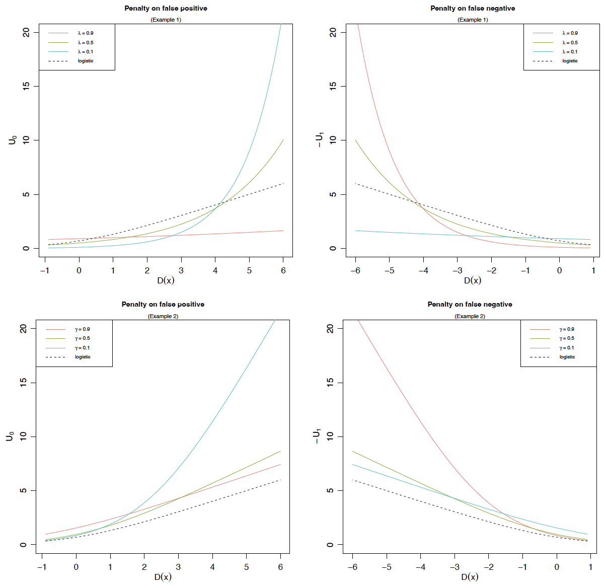
In Examples 1 and 2, the tuning parameter, $\lambda$ in (2.6) and $\gamma$ in (2.7), balances the penalties on false positive and false negative predictions, which ensures that the LCMs are flexible enough to meet a specific target on FPR or FNR. To illustrate this point, let us compare the weighting function $w$ given by (2.6) or (2.7) with the logistic weighting function in (2.8) and plot in Figure 1 the penalties as a function of the linear predictor $\mathcal{D}(x)$ defined by (2.1) under different $w$. In Figure 1, the $y$-axis is the corresponding penalty, measured by $U_0(\mathcal{D}(x))$ on false positive predictions in the left panel and by $-U_1(\mathcal{D}(x))$ on false negative predictions in the right panel. An immediate observation is that the value of $\lambda$ in (2.6) or $\gamma$ in (2.7) controls the degree of penalty on false positive and false negative cases, exactly as we claimed. When $\lambda$ or $\gamma$ increases, the penalty on false positive decreases, but the penalty on false negative increases for large values of $\mathcal{D}(x)$. As a result, if we want to achieve a small FPR, we should select a small $\lambda$ in (2.6) or $\gamma$ in (2.7), and vice versa. We further observe that, in the limit case of $\lambda \to 0$ (respectively, $\lambda \to 1$), the corresponding right (respectively, left) tail exhibits exponential growth. As a comparison, when the logistic weighting function (2.8) is used, the penalties on false positive and false negative are symmetric and have linear growth. (Similar results apply to the weighting function in (2.7) with $\gamma$ being the tuning parameter; see lower panels in Figure 1.) Such a difference is key to achieving a target on FPR or FNR under the LCMs.

2.2. Calibration

We next discuss how to calibrate an LCM with training data. For such a purpose, we first choose a weighting function $w$, which determines two penalty functions $U_0$ and $U_1$ by (2.3) and in turn determines the loss function $\mathcal{L}$ by (2.2). Next, we minimize the loss function $\mathcal{L}$ to obtain the estimates of estimate $\boldsymbol{\theta}:=(\alpha, \beta)$. Since $\mathcal{L}$ is differentiable, we attempt to find the estimates by solving the following equation from the first-order condition (FOC):

$$\begin{aligned} \frac{\partial}{\partial\boldsymbol{\theta}} \mathcal{L}(\boldsymbol{\theta})=0. \end{aligned}$$

As an illustrative example, let us consider the exponential weighting function $w$ given by (2.6), in which $\lambda \in (0, 1)$ is a tuning parameter. Now by using (2.6), we can simplify the above FOC equation into

$$\scriptsize{\begin{aligned} \frac{\partial}{\partial\boldsymbol{\theta}} \mathcal{L}(\boldsymbol{\theta}) &= \lambda(1-\lambda)\sum_{i=1}^n \left( (1-Y_i) \, \mathrm{e}^{(1-\lambda)\mathcal{D}(x_i)}- Y_i \, \mathrm{e}^{-\lambda\mathcal{D}(x_i)}\right) x_i\\ & = 0, \end{aligned} \tag{2.9}}$$

in which $\mathcal{D}(x) = \alpha + \beta^\top x$ is defined in (2.1). A solution to (2.9), denoted by $\hat{\boldsymbol{\theta}} = (\hat{\alpha}, \hat{\beta})$, is indeed the minimizer of the loss function $\mathcal{L}$ because the determinant of the corresponding Hessian matrix $\frac{\partial^2}{\partial\boldsymbol{\theta}^2} \mathcal{L}(\boldsymbol{\theta})$ is

$$\small{\begin{aligned} \lambda(1-\lambda)\sum_{i=1}^n x_i^\top \left( (1-Y_i)(1-\lambda) \, \mathrm{e}^{(1-\lambda)\mathcal{D}(x_i)}+ \lambda Y_i \, \mathrm{e}^{-\lambda\mathcal{D}(x_i)}\right) x_i > 0, \end{aligned}}$$

for all $\lambda \in (0,1)$.

Since the logistic model is a special LCM with the weighting function $w$ given by (2.8), we can follow the same procedure to estimate $\boldsymbol{\theta}$ under the logistic model. To be precise, the corresponding FOC equation reads as

$$\begin{aligned} \frac{\partial}{\partial\boldsymbol{\theta}} \mathcal{L}(\boldsymbol{\theta})=\sum_{i=1}^n \left(-Y_i + \frac{\mathrm{e}^{\mathcal{D}(x_i)}}{1+ \mathrm{e}^{\mathcal{D}(x_i)}}\right) x_i =0 . \end{aligned}$$

In this case, the FOC is sufficient as we verify

$$\begin{aligned} \left| \frac{\partial^2}{\partial\boldsymbol{\theta}^2} \mathcal{L}(\boldsymbol{\theta}) \right| =\sum_{i=1}^n x_i^\top \left( \frac{\mathrm{e}^{\mathcal{D}(x_i)}}{(1+ \mathrm{e}^{\mathcal{D}(x_i)})^2}\right) x_i>0. \end{aligned}$$

3. Simulation study

In this section, we conduct a simulation study to assess the applicability of the LCMs introduced in Section 2. We will consider all three weighting functions introduced in Examples 1–3 and study their performance in classification, with the logistic weighting function in (2.8) of Example 3 serving as the benchmark.

What we have in mind is a risk classification problem in automobile insurance with two classes, in which class $Y=0$ represents a standard risk and class $Y=1$ denotes a substandard risk. Because of the extreme imbalance between the two classes (see So, Boucher, and Valdez 2021), we consider an insurance pool of $n_0 = 10,000$ standard risks $(Y=0)$ and $n_1 = 500$ substandard risks $(Y=1)$. For illustration purposes, assume there are two covariates, $X_1$ and $X_2$, in this study; $X_1$ relates to the driver’s age (in the unit of 10 years), and $X_2$ corresponds to the (rescaled) vehicle capacity. We use the following conditional distributions of $(X_1, X_2)| Y$ to generate data:

$$\begin{aligned} (X_1, X_2) \big| Y=0 \sim \mathcal{N}\left(\mu_{0}, \, \Sigma_{0} \right), \end{aligned}$$

in which

$$\begin{aligned} \mu_{0}=\begin{pmatrix}4.95 \\ 1.5\end{pmatrix} \quad \text{and} \quad \Sigma_{0}= \begin{pmatrix} 1 & 0 \\ 0 & 0.3 \end{pmatrix}, \end{aligned}$$

and

$$\begin{aligned}(X_1, X_2) \big| Y=1 \sim \mathcal{N}\left(\mu_{1}, \, \Sigma_{1} \right),\end{aligned}$$

in which

$$\small{\begin{aligned} \left[ \mu_1, \Sigma_1 \right] = \begin{cases} \left[\begin{pmatrix}4.95 \\ 2.2\end{pmatrix}, \begin{pmatrix} 0.5 & 0 \\ 0 & 0.3 \end{pmatrix}\right], & \text{ with probability } 0.1, \\ \left[\begin{pmatrix}2.5 \\ 2.6\end{pmatrix}, \begin{pmatrix} 0.2 & 0 \\ 0 & 0.1 \end{pmatrix}\right], & \text{ with probability } 0.9. \end{cases} \end{aligned}}$$

In the above, $\mathcal{N}(\mu, \Sigma)$ denotes a (bivariate) normal distribution with mean $\mu$ and variance-covariance matrix $\Sigma$. Let us explain the above distributions of the covariates $(X_1, X_2)$ given $Y = 1$ as follows. For the simulation study, we expect that a smaller $X_1$ (younger age) or a larger $X_2$ (bigger vehicle) should yield a higher risk score. In that sense, most of the substandard risks should have younger ages, when compared with the standard risks; this explains why we set the mean $\mu_1$ to 2.5 (i.e., 25 years of age) with probability of 0.9, which is significantly smaller than $\mu_0 = 4.95$ for standard risks. Conversely, as one ages beyond a certain threshold, the chance of being flagged as a substandard risk increases. To reflect this fact, we set the second scenario of $\mu_1$ to be equal to $\mu_0 = 4.95$ with probability of 0.1. Because of the above choice of $[\mu_{1}, \Sigma_{1}]$, some of the substandard risks are mixed together with the standard risks, as shown in Figure 2, which makes classification a challenging task.

Figure 2.Joint scatter plot of $(X_1)$ and $(X_2)$.

Figure 3.Trade-off between FPR/TPR and FNR/TNR in the simulation study with $\mathbb{P}(Y=0) \approx 95\%$.

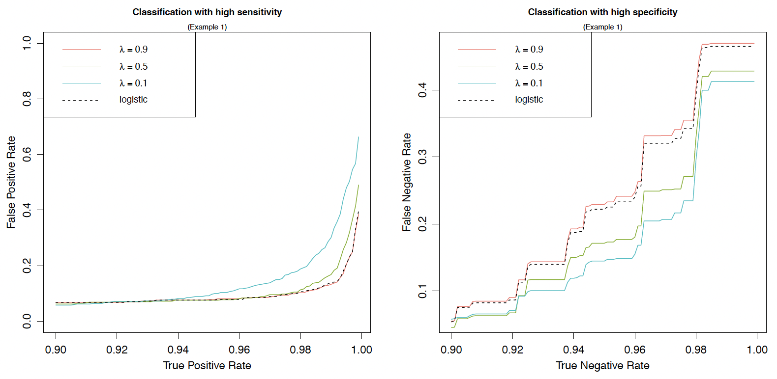
Recall that we consider three weighting functions from Examples 1–3 in the study: the first two choices are parameterized by $\lambda$ in (2.6) or by $\gamma$ in (2.7), and the last one in (2.8) corresponds to the standard logistic model. As shown in Figure 1, a larger $\lambda$ or $\gamma$ places more penalty weight on FPR in the loss function $\mathcal{L}$. We compare the performance when $w$ is given by (2.6), (2.7), or (2.8) and plot the findings in the region of high sensitivity and high specificity in Figure 3. Note that “high sensitivity” refers to situations in which an insurer prefers a high true positive rate (TPR) or equivalently a low FNR. (TPR is defined by $\frac{\text{TP}}{\text{TP + FN}}$ and equals $1 - \text{FNR}$; see Table 1.) Conversely, “high specificity” corresponds to situations in which an insurer aims for a high true negative rate (TNR) or equivalently a low FPR. (TNR is defined by $\frac{\text{TN}}{\text{TN + FP}}$ and equals $1 - \text{FPR}$; see Table 1.) In the high-sensitivity region (two left panels in Figure 3), the $x$-axis is the TPR, ranging from 90% to 100%, while the $y$-axis denotes the corresponding FPR under a given TPR. The two right panels in the high-specificity region can be understood in a similar way. Therefore, in all panels of Figure 3, the lower the curve, the better is the performance. It is worth mentioning that the plots in Figure 3 are not ROC curves, which are plots of TPR as a function of FPR.

Let us first focus on the upper panels of Figure 3 in the case of the exponential weighting function given by (2.6) in Example 1. An important observation is that the LCMs with $w$ given by (2.6) can outperform the benchmark logistic regression model by choosing an appropriate $\lambda$; such a result is more evident in the region of high sensitivity than in the region of high specificity. The upper left panel shows that, given a target TPR (between 90% and 100%), a larger $\lambda$ yields a lower FPR in most scenarios and is thus generally preferred to the insurer. On closer investigation of different $\lambda$ values (not shown here), we find that LCMs with exponential weighting outperform the benchmark logistic model for $\lambda > 0.2$ in the high-sensitivity region. Moving to the upper right panel, we find that the FNR overall increases with respect to $\lambda$ for a given target TNR (between 90% and 100%) and that, to outperform the benchmark, the insurer needs to choose $\lambda \le 0.1$. When the weighting function is given by (2.7), as in the two lower panels, findings similar to those above can be drawn, although the plots are less distinguishable compared to those in the upper panels.

We further observe from Figure 3 that the logistic regression model performs poorly in the high-sensitivity region but delivers good performance in the high-specificity region. The reason for the latter result is that the generated dataset is heavily imbalanced, with about $95\%$ of observations in the class $Y=0$ (i.e., the actual negative rate is $\frac{10,000}{10,000 + 500} \approx 95\%$), and the TNR is between 90% and 100% in the high-specificity region. In other words, the high-specificity region in Figure 3 represents the simulated dataset well, and under such a scenario, which is of course not always true in real applications, the good performance from the logistic regression model is expected. To further illustrate this point, we consider a “reversed” dataset compared to the previous one, in which we relabel the 500 risks in the minority class as $Y=0$ (“negative”) and the 10,000 risks in the majority class as $Y=1$ (“positive”). As a result, this reverse dataset has an actual positive rate of 95% and thus is approximated well by the high-sensitivity region, which has a TPR between 90% and 100%. Our previous claim then predicts that the logistic regression model will deliver good performance in the high-sensitivity region but not in the high-specificity region for the reversed dataset with $\mathbb{P}$(“positive”) $\in (90\%, 100\%)$. This prediction is exactly what Figure 4 implies. As a comparison, LCMs under the exponential weighting function still can deliver excellent performance in the high-specificity region when a small $\lambda$ is chosen; indeed, those with $\lambda < 0.6$ outperform the benchmark logistic model. To summarize, LCMs with suitable parametric weighting functions (e.g., Examples 1 and 2) can be effectively tuned to achieve excellent performance in either the high-sensitivity or the high-specificity region, whereas the benchmark logistic model performs well only in the region that is representative of the actual data.

Figure 4.Trade-off between FPR/TPR and FNR/TNR in the simulation study with $\mathbb{P}(Y=1) \approx 95\%$.

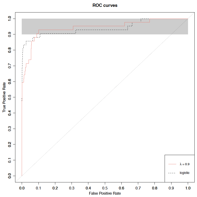
Recall that the graphs in Figure 3 are plotted for high sensitivity (i.e., high TPR) or high specificity (i.e., high TNR) between 0.90 and 1.00. As such, the findings above are for those regions only and may not hold over the entire region when TPR or TNR is between 0 and 1. To have an overview of the performance, we consider two LCM models: the first model has an exponential weighting function with $\lambda = 0.9$, and the second model is the logistic model with $w$ given by (2.8). We plot the ROC curves for these two models in Figure 5. We easily observe from Figure 5 that the first model with $\lambda = 0.9$ outperforms the logistic model in the gray-shaded region, which has a TPR between 0.9 and 1 and corresponds to the high-sensitivity region in Figure 3. In that regard, Figures 3 and 5 offer consistent findings.

Figure 5.ROC curves when $w$ is given by (2.6) with $\lambda = 0.9$ and by (2.8).

To gain a more accurate comparison of different models over the entire region, a better choice is the AUC, which can be understood as a measure of the probability of correct classifications and is thus always between 0.0000 and 1.0000. For a classifier, the higher the AUC, the better is its performance. A perfect classifier yields an AUC of 1, while an uninformative classifier produces 0.5, which is the area under the diagonal line. We calculate the AUC for the LCMs under different $\lambda$ or $\gamma$ and for the logistic model in Table 2. We find that all models, including the benchmark logistic model, perform well, with AUCs all larger than 0.97. However, the parametric models with $\lambda$ or $\gamma$ greater than 0.5 still can outperform the logistic model.

The results from the simulation study above show that LCMs with parametric weighting functions given by (2.6) or (2.7) have a twofold advantage over the benchmark logistic model. First, they are highly flexible and can be tuned by users to achieve a specific target on FPR or FNR while the benchmark logistic model cannot. Second, they can always outperform the benchmark logistic model under an appropriate tuning parameter.

3.1. Discussion about hyperparameter selection

We consider LCMs with parametric weighting function $w$ for their tractability and applicability. Examples 1 and 2 present two useful choices for such a $w$, in which the hyperparameter $\lambda$ or $\gamma$ plays a key role in the prediction performance. A natural question then is how to select the hyperparameter(s) of the weighting function $w$. The goal of this subsection is to offer discussion about this question when $w$ is given by the exponential weighting function of Example 1 (Example 2 or other parametric weighting functions can be analyzed similarly).

First, we observe an approximately increasing (respectively, decreasing) relationship between $\lambda$ and performance in the high-sensitivity region (respectively, high-specificity region); see Figure 3. It is worth pointing out that such a result holds true in general; indeed, the same observation holds in the empirical analysis (see Figure 8). As such, this result offers important guidance about selecting the parameter $\lambda$.

Continuing the above discussion, we know that insurers should use small $\lambda$ in the high-specificity region or large $\lambda$ in the high-sensitivity region. Using the training data and considering several $\lambda$ can reveal more useful information. As an example, by considering $\lambda = 0.1, 0.5, 0.9$, the above simulation study indicates that insurers should choose $\lambda \le 0.1$ to outperform the logistic model in the high-specificity region. Conducting such a comparison analysis gives an approximate range for the hyperparameter once insurers set their target TNRs or TPRs. However, the specific result (for example, $\lambda \le 0.1$ in this case) may depend heavily on the training data and should not be taken as a universal rule.

With the above problem in mind, we proceed to discuss how the idea of cross-validation can be applied to select a suitable tuning parameter for an LCM. To be precise, the procedure of selecting a suitable $\lambda$ consists of the following four steps:

1. Fix a value function (performance measure) $V(\alpha, \beta|{D})$^[3] in which $\alpha$ and $\beta$ are from (2.1) and ${D}$ is the validation dataset.

2. Split the training dataset into $K$ parts (a usual choice is $K=5$ or $10$); set aside the $k^{th}$ part, denoted by ${D}^{(k)}$, for the cross-validation purpose; and use the remaining $K-1$ parts, denoted by $D^{(-k)}$, to calibrate the model.

3. For $k=1,\ldots,K$, we first use the dataset $D^{(-k)}$ to obtain the estimates for $\alpha$ and $\beta$, denoted by $\hat{\alpha}^{(k)}$ and $\hat{\beta}^{(k)}$, respectively, and then compute $V\big(\hat{\alpha}^{(k)}, \hat{\beta}^{(k)} \, | \, D^{(k)} \big)$.

4. Define the average value function $\overline{V}$ by

   $$\bar{V}(\lambda):=\frac{1}{K} \sum_{k=1}^K V\left(\hat{\alpha}^{(k)}, \hat{\beta}^{(k)} \mid D^{(k)}\right). \tag{3.1}$$

   A suitable choice for the hyperparameter $\lambda$ is then the maximizer, denoted by $\lambda^*$, of $\overline{V}$, i.e.,

   $$\lambda^*=\arg \max _\lambda \bar{V}(\lambda). \tag{3.2}$$

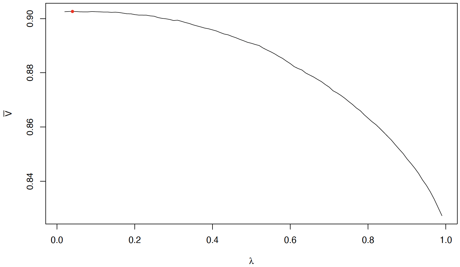
The approach above for selecting a $\lambda$ is general enough to be applicable in most cases. However, two difficulties remain in actual applications. First, what kind of $V$ (performance measure) should we use? Second, how do we solve the optimization problem in (3.2), which is often nonsmooth and nonconcave? Both problems are well known and can be very challenging, and so far neither has a generally accepted solution. That said, we will not attempt to address either problem in this article because such a task goes far beyond the scope of the current work. Nevertheless, we will conduct an illustrative example using the same simulation dataset to demonstrate the potential use of the above procedure. For that purpose, we assume that the insurer is interested in the high-specificity region (with $\text{TNR} \in [0.9, 1]$) and adopts the following value function $V$:

$$\scriptsize{V(\alpha, \beta|{D})=\frac{1}{100}\sum_{i=1}^{100} \mathbb{P}(\hat{Y}=1|Y=1, \text{TNR}=0.9+\frac{i}{1000}; \alpha, \beta | {D}).} \tag{3.3}$$

Note that in (3.3), each probability is the conditional probability of correctly classifying a substandard risk under a targeted TNR between 0.90 and 1.00. As a result, maximizing $\overline V$ in (3.1) is consistent with the insurer’s business target of a high TNR. To find the maximizer $\lambda^*$ as defined in (3.2), we conduct a naïve grid search over $0.01, 0.02, \dots, 0.98, 0.99$ (with a step size of 0.01 over $(0,1)$) and plot $\overline V$ as a function of $\lambda$ in Figure 6. We find that the maximizer $\lambda^*$ is 0.04, which is less than 0.1, as previously suggested by Figure 3.

Figure 6.$\overline{V}$ in (3.1) as a function $\lambda \in(0,1)$.

4. Empirical analysis

In this section, we continue to apply the LCMs to study risk classification problems in insurance and assess their performance. However, in contrast to the simulated study with simplified covariates in the previous section, we will use the LGPIF data (publicly available at https://sites.google.com/a/wisc.edu/jed-frees/#h.lf91xe62gizk), collected in the state of Wisconsin, to conduct an empirical analysis. For an overview of this dataset, see Frees, Lee, and Yang (2016); recent actuarial applications using this dataset can be found in Lee and Shi (2019), Jeong and Zou (2022), and Jeong, Tzougas, and Fung (2023), among others. In Section 3, we considered the LCMs under two parametric weighting functions, (2.6) and (2.7), and they deliver similar performances in terms of AUC (see Table 2). However, Figure 3 suggests that the models with (2.6) are more flexible than those with (2.7) in the high-sensitivity and high-specificity regions. In addition, the penalty functions $U_0$ and $U_1$ are more tractable under (2.6) than under (2.7), as shown in Examples 1 and 2. As such, we will focus on the exponential weighting function (2.8), along with the logistic weighting function (2.6), in the empirical study. Recall that $\lambda \in (0,1)$ is the tuning parameter in (2.6); similar to what we did in Section 3, we consider three levels for $\lambda$ at 0.1, 0.5, and 0.9. For convenience, we will refer to the LCMs with exponential weighting as exponential LCMs in this section.

4.1. Data description and calibration

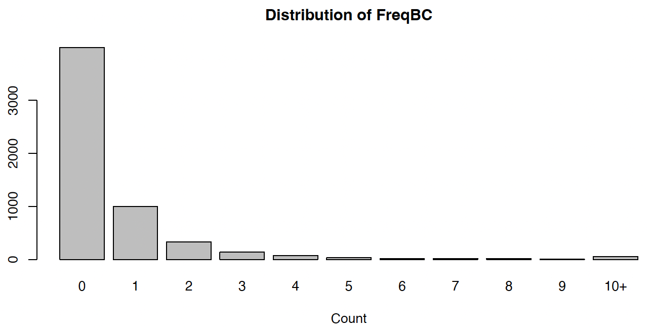
While the LGPIF dataset provides information about policy characteristics and claims on multiple lines of coverage, we focus on the BC coverage in the empirical analysis. The dataset has a total of 6,775 observations that are recorded from 2006 to 2011; we will use the 5,677 observations from 2006 to 2010 as the training set to calibrate the classification models and the remaining 1,098 observations from 2011 for out-of-sample validation. There are seven categorical covariates and two continuous covariates, as seen in Table 3; since a policy is assigned a “type” from the available six categories, one type covariate is redundant, and thus the covariates vector $X$ is of dimension $d=8$. The response variable is the number of BC claims in a year. Summary statistics of the observed policy characteristics and the claim counts in the training set are provided in Table 3.

Figure 7.Distribution of FreqBC in the training set.

As shown in Figure 7, most policyholders did not file a claim within a year, but there are still some policyholders who filed multiple claims within a year. There are 11 classes (with claim number $N = 0,1,\cdots, 10+$) in Figure 7, and the linear classification framework is for a binary problem, so it is necessary to select a threshold $h$ for the claim number $N$ and divide all policies into two classes. Once $h$ is selected, we define the majority class $Y = 0$ and the minority class $Y = 1$ by

$$\small{\begin{aligned} \{ Y = 0\} = \{ N \le h\} \quad \text{and} \quad \{Y = 1\} = \{N > h\}, \end{aligned}}\tag{4.1}$$

in which $N$ denotes the number of claims filed in a year. For robustness concern over the choice of $h$, we will consider four thresholds, $h = 1,2,3,4$, in the analysis.^[4]

Following the procedure documented in Section 2.2, we calibrate the exponential LCMs under different $\lambda$ by using the observations from 2006–2010 in the LGPIF dataset. The estimated model parameters, $\hat{\alpha}$ and $\hat{\beta}$ (see (2.1) for the meanings of $\alpha$ and $\beta$), are presented in Table 4. For each column in Table 4 under a given threshold $h$ (see (4.1) for the meaning of $h$), the value in the “(Intercept)” row is the estimated $\hat{\alpha}$, and the value under each covariate corresponds to the estimated component of $\hat{\beta}$ for that covariate where $Y$ is defined accordingly. All the estimates for the logistic regression model are close to those under the exponential LCM with $\lambda = 0.1$. Detailed discussions about $\hat{\alpha}$ and $\hat{\beta}$ follow.

• Discussion about $\hat{\alpha}$: The exponential LCM with $\lambda = 0.9$ has the largest $\hat{\alpha}$ among the four models considered. Furthermore, $\hat{\alpha}$ decreases first and then increases when $\lambda$ increases from 0.1 to 0.9, exhibiting a convex shape with steeper growth for larger $\lambda$ values. Comparing across choices of the threshold $h$, we find that $\hat{\alpha}$ is the smallest when $h = 4$ but that there is no obvious relation between $\hat{\alpha}$ and $h$.

• Discussion about $\hat{\beta}$: Recall that there are eight covariates in $X$. The first six are categorical variables, and the last two are the continuous variables with their names in the first column of Table 4. For convenience, let us denote $\hat{\beta}_i$, the estimated $\beta_i$ for the $i$th covariate variable, where $i = 1,\cdots,8$. The first important observation is that most $\hat{\beta}_i$s have the same sign for all four models. Note that for a given $X_i$, a positive $\hat{\beta}_i$ means the larger the $X_i$ of a policy, the more likely it is that the policy is classified as a substandard risk. As such, the estimation results overall are consistent with our intuition. For instance, $\hat{\beta}_7>0$ and $\hat{\beta}_8 < 0$ imply that a larger coverage $(X_7)$ or a smaller deductible $(X_8)$ is riskier to the insurer.

4.2. Results

With the model parameters calibrated in Table 4, we are now ready to investigate the performance of the four models (see Table 4 in the empirical study). Note that all four models belong to the LCM family introduced in Section 2: the first three models are under the exponential weighting function (2.6) but with different $\lambda$, and the last one is the logistic regression model with $w$ given by (2.8). We use the observations from 2011 to conduct out-of-sample validation to evaluate the performance of those four models.

Recall that high specificity is associated with high TNR and high sensitivity is associated with high TPR, both from 0.90 to 1.00 in our examples, as in Figure 3. Since achieving high TNR often conflicts with achieving high TPR, just as when minimizing Type I and Type II errors, we need to decide which target is preferred in the study. In insurance underwriting, if an insurer adopts a strategy with high sensitivity, that means the insurer is willing to accept all applications, except those deemed too risky. For the LGPIF dataset, the fund is set to provide affordable and accessible insurance for state-owned properties, and the State of Wisconsin acts as the public insurer. Therefore, it is clear that we should aim for high TPR and focus on model performance in the high-sensitivity region in our empirical study.

Figure 8.Trade-offs between FPR/TPR under different $h$ with the LGPIF dataset.

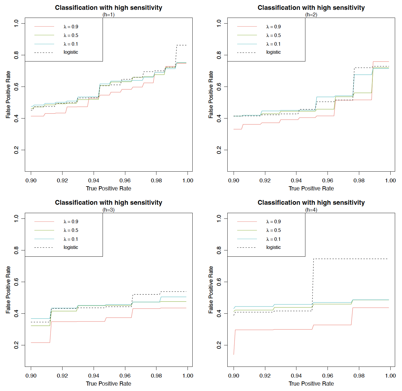
We plot FPR against TPR in the high-sensitivity region with TPR between 0.90 and 1.00 for all four models in Figure 8; each panel corresponds to a particular choice of $h$, which defines the majority and minority classes by (4.1). For the three exponential LCMs, we observe an overall decreasing relation between FPR and the tuning parameter $\lambda$, i.e., a larger $\lambda$ leads to a smaller FPR in most scenarios and is thus more preferred to the insurer. Indeed, the model with $\lambda = 0.9$ has the best performance, in terms of FPR, among all four models; in particular, it outperforms the benchmark logistic regression model by a significant margin for all choices of the threshold parameter $h$. Also, the exponential LCMs are more robust than the logistic model with respect to $h$.

We next study model performance over the entire region instead of the high-sensitivity region with TPR between 0.90 and 1.00. To that end, we use the AUC measure and calculate it for all four models in Table 3. While all four models show satisfactory classification performance overall with AUC larger than 0.8, it is clear that the exponential LCM with $\lambda = 0.9$ is the best one. This is partially due to its superior performance in the high-sensitivity region. We also see an increasing relationship between AUC and the threshold parameter $h$. As is clear from Figure 8, when $h$ increases from 1 to 4, the probability of the minority class $(\{ Y = 1 \} = \{N > h\})$ decreases quickly to near 0, which naturally leads to a much easier classification task and a larger AUC value.

5. Conclusions

We apply the LCMs of Eguchi and Copas (2002) under a flexible loss function to study binary classification problems. There are two penalty terms in the loss function: the first term penalizes false positive cases, and the second term penalizes false negative cases. Under reasonable conditions, the loss function can be represented uniquely by a positive weighting function $w$, and its choice determines the impact of false positive and false negative on classification. The choice for such $w$ is unlimited, and we introduce two parametric families that both are tractable and easily can be tuned to meet targeted rates on false positive or false negative. The first one is proposed in Eguchi and Copas (2002), and the second one is new, to our awareness. We also show that one particular choice of $w$ recovers the standard logistic regression model, making it a special case nested under the LCMs.

To illustrate the usefulness of the LCMs in actuarial applications, we consider both a simulated study and an empirical analysis. The simulated study is based on a highly imbalanced dataset related to risk classification in automobile insurance, and the results show that the LCMs under the two parametric weighting functions in Examples 1 and 2 can always outperform the logistic regression model in both the high-sensitivity and high-specificity regions and also under the AUC measure. Moreover, those models show great flexibility, upon the choice of an appropriate tuning parameter, to achieve a target rate on false positive or false negative predictions. The empirical analysis uses the LGPIF dataset and focuses on the prediction of claim frequency $N$ (per year). We first select a threshold parameter $h\ (h=1,2,3,4)$ and divide $N$ into two classification classes $\{N \le h\}$ and $\{N > h\}$. The promising findings from the simulated study apply in a parallel way to the empirical study; the LCMs under the exponential weighting function in (2.6) can be tuned to outperform the logistic model. Furthermore, the outstanding classification performance is robust to the choice of the threshold parameter $h$.

Electronic Supplementary Material

The R codes for simulation and empirical data analysis are available at https://github.com/ssauljin/linearscore.

Acknowledgments

We thank the editor and two reviewers for insightful comments and suggestions that helped improve the quality of the article. We kindly acknowledge the financial support of a 2022 Individual Research Grant from the CAS.