Accounting for Model Risk in Property and Casualty Insurance

undefined

1. Introduction

Model risk occurs when a financial institution’s model does not accurately describe the actual risk. It is broader than estimation risk, which occurs when parameter estimates are subject to sampling uncertainty owing to the data’s finite sample size despite an assumed well-specified model. Conversely, model risk includes additional risk that results from a financial institution’s fundamentally misspecified model, which affects both the risk prediction and its associated uncertainty. Therefore, it must be accounted for in both pricing and risk management.

Model risk has recently received much attention in the finance/insurance field, especially in relation to market risk (Morini 2011; Alexander and Sarabia 2012; Glasserman and Xu 2014; Bertram, Sibbertsen, and Stahl 2015; Danielsson et al. 2016; Lazar and Zhang 2022). Many regulators have also published guidelines for integrating model risk into financial institutions’ risk management processes. However, a solid framework is lacking for retail individual-level risks, with even less of a framework available for the property and casualty insurance domain. Supposing that we had policy-level data on an insurance portfolio and one or more competing models, how could we adjust the prediction for model risk and quantify the prediction’s uncertainty, given that the model we use is not necessarily well specified?

The insurance literature has proposed two approaches to model risk. The first is mainly theoretical and is motivated by risk aggregation at the company level when the risk distribution is known for each business line. For instance, Embrechts, Puccetti, and Rüschendorf (2013), Bernard, Jiang, and Wang (2014), and Bernard, Rüschendorf, and Vanduffel (2017) identified bounds for the value at risk of the aggregate loss \(Y_1+Y_2+\cdots Y_n\), if the marginal distributions of line-by-line losses \(Y_1\), …, \(Y_n\) are given, but the dependence between them is not fully known. Fadina, Liu, and Wang (2024) studied the impact of model uncertainty on risk measures. However, this setting is less relevant for pricing individual risks.

The other approach is based on Bayesian model averaging, first introduced in statistics by Raftery, Madigan, and Hoeting (1997). Typically, prior probabilities are first assigned to a set of competing models, then the Bayes formula is used to compute the models’ posterior probabilities. This latter distribution can then be used to select the most likely model or to compute the average prediction (Cairns 2000; Peters, Shevchenko, and Wüthrich 2009; Hartman and Groendyke 2013; Barigou et al. 2023; Jessup, Mailhot, and Pigeon 2023). The downsides of this approach are threefold. First, like any other Bayesian approach, the posterior distribution is sensitive to the prior probabilities choice. Second, existing literature implicitly assumes that one of the candidate models is correctly specified, which has implications for both risk prediction and model selection. For prediction, this assumption could lead to systematic bias in the prediction, if, for instance, all candidate models underestimate the risk. For selection, this assumption could result in the best model being overlooked. In cases where one model nests another, the more flexible nesting model tends to be prioritized by the posterior distribution, since it usually provides a better fit than the constrained nested model. In other words, the Bayesian model averaging approach does not account for the number of parameters, which implies a risk of overfitting (Florens, Gouriéroux, and Monfort 2019). Third, the standard frequentist selection rules based on the Akaike information criterion (AIC) and the Bayesian information criterion (BIC) also do not account for model risk. Moreover, these selection rules are only asymptotically consistent (Florens, Gouriéroux, and Monfort 2019) under the assumption that one of the candidate models is actually correct. In other words, with a finite sample size or when no candidate models are correctly specified, the probability of selecting the best model is strictly smaller than one.

To the best of our knowledge, quantifying model risk using individual-level property and casualty insurance data has yet to be investigated. The research closest to our aim is that of Gouriéroux and Monfort (2021) (henceforth, GM), which investigated retail credit risk applications. The authors’ premise was that, although the “true” model is fundamentally unobservable, it is possible to quantify the impact of the misspecification risk on some low dimensional summary statistics if we have an additional out-of-sample validation population. In credit risk, the low dimensional summary statistics often comprise the total loss from loan defaults. The authors explained \((i)\) how to compute the potential bias of each given model and \((ii)\) when a loss function is used to choose between several competing models, how the model risk of each model needs to be accounted for.

While the GM work considered credit risk, applying their framework to insurance is not straightforward for several reasons. First, the research was mainly theoretical (see however, Gouriéroux and Tiomo 2019 for a partial application of their methodology to confidential credit data). Second, property and casualty insurance variables (mostly frequency or severity) differ from those of credit risk (mostly a binary default indicator and a continuous loss-given-default measure). Third, some statistical terminologies used in their paper, such as pseudo model, are not yet popular among the actuarial community. Fourth, their research focused on parametric models only, and they did not address its applicability to machine learning methods. We solved these issues by \((i)\) providing illustrations using both simulated count data and real insurance data; \((ii)\) starting with classical generalized linear models to illustrate some of GM’s concepts; and \((iii)\) incorporating machine learning methods, such as XGBoost.

The rest of the paper is organized as follows. Section 2 discusses the methodology of accounting for model risk in prediction models. Section 3 applies this methodology to simulated data. Section 4 discusses the methodology for taking model risk into account for model comparisons. Section 5 illustrates this methodology using the same simulated data. Section 6 applies the methodologies from Sections 2 and 4 to a real dataset. Section 7 concludes the paper.

2. Accounting for model risk in prediction: Methodology

2.1. Setting

Suppose that the insurer has two databases, one training (i.e., estimation) sample with \(n\) policies, henceforth called the sample, and one out-of-sample dataset with \(N\) policies, called a validation or prediction population. This assumption is valid because a single database can be randomly split into a training database and an out-of-sample database. Both \(n\) and \(N\) are large but finite, with comparable orders of magnitude. That is, \(\frac{N}{n} \approx {\mu}\) is a constant. We denoted the vector of covariates by \(X_i, i=1,...,n\), and the response variable for policy \(i\) in the training sample by \(Y_i, i=1,...,n\). We focused on the case with a frequency (count) response variable, but the same methodology can be applied to the case where the response variable is the total claim cost of a policy. We denoted the counterparts in the validation population by \(X_k, Y_k, k=1,...,N\), respectively. Throughout the study, we used index \(i\) (respectively, \(k\)) when variables \(X\) and \(Y\) were from the sample (respectively, population). We also assumed that \((X_i, Y_i)\) in the sample and \((X_k, Y_k)\) in the population were all independent and identically distributed random variables (i.i.d.).

We assumed that for the sample, both \(X_i\) and \(Y_i\), \(i=1,...,n\), were observed, whereas for the population, we assumed that \(X_k, k=1,...,N\) were observed, but the observability of \(Y_k\) depended on the type of application. This section of the study focused on predicting the average total claim cost or count on the population, i.e., \(\frac{1}{N}\sum_{k=1}^N Y_k\), and its associated 95% confidence level. For this purpose, we did not require \(Y_k\) to be observed. In a later section we focused on two types of model comparison. In the first type, the population was an outstanding portfolio for which \(Y_k\) was unobserved, then we compared the prediction of \(\frac{1}{N}\sum_{k=1}^N Y_k\), obtained using different models, to assess whether one model produced predictions that were significantly larger than those of competing models. In this case, we did not require the observation of \(Y_k\) in the population. In the second type, the population was used for validation purposes, so our aim was to choose the model that best fit the data, then we assumed that \(Y_k\) was observed in the validation population as well, to compare with predictions obtained from different models.

2.2. Methodology

To illustrate the importance of accounting for model risk and to emphasize how it differs from estimation risk, we considered three cases. The toy case assumed that the actuary completely ignored both the model risk and the model estimation risk. In other words, the actuary assumed (wrongly) that the used model was the true model. The intermediate case assumed that the actuary accounted for the model estimation risk in a classical parametric framework but did not account for the model risk. Finally, in the most realistic case, the actuary accounted for both risks, regardless of whether a parametric or machine learning model was used.

Toy case: The estimated model was wrongly believed to be the true model. Under this scenario, the actuary assumed they knew exactly the data generating process (DGP) and that the parameter \(\hat{\theta}\) estimate was equal to its true value \(\theta_0\). We denote by \(C(X, \theta_0):=\mathbb{E}[Y|X]\) the conditional prediction under the true model and \(\sigma^2(X, \theta_0):=\mathbb{V}[Y|X]\) the conditional variance. Then, by the central limit theorem, the \(95\%\) confidence interval of \(\frac{1}{N}\sum_{k=1}^N Y_k\) is asymptotically:

\[ \Big(\frac{1}{N}\sum_{k=1}^N C(X_k, \hat{\theta}) \pm \frac{1.96}{\sqrt{N}} \sqrt{\frac{1}{ {N}}\sum_{k=1}^N \sigma^2(X_k, \hat{\theta}) }\Big).\tag{1} \]

Intermediate case: The true model is still assumed known, its parameter \(\theta_0\) must be estimated using the training sample, but this time the estimation uncertainty was accounted for. We denote by \(\hat{\theta}\) such an estimator and assume that \(\hat{\theta}\) converges to its true value \(\theta_0\) as the sample size \(n\) increases to infinity, with an asymptotic normal distribution:

\[ \sqrt{n} (\hat{\theta} -\theta_0) \longrightarrow \mathcal{N}(0, V_{as}(\hat{\theta})), \tag{2} \]

where \(V_{as}(\hat{\theta})\) is the asymptotic variance matrix of the rescaled estimator \(\sqrt n \hat\theta\).

Such an assumption is satisfied by usual estimators of most parametric models. For instance, it is well known that the maximum likelihood estimator (MLE) is usually consistent and asymptotically normal. Moreover, if \(\hat\theta\) is the MLE, then matrix \(V_{as}(\hat{\theta})\) is simply the inverse of the Fisher’s information matrix.

From here forward, we assume that matrix \(V_{as}(\hat{\theta})\) can be consistently estimated using the training sample. We denote such an estimator by \(\hat{V}(\theta)\). For instance, in the case of MLE, we can use the inverse of the sample information matrix as the estimator of \(V_{as}(\hat{\theta})\).

In this intermediate case, the theoretical prediction (1) cannot be computed, since the insurer does not observe \(\theta_0\) but only its estimator \(\hat{\theta}\). In other words, \(\frac{1}{N}\sum_{k=1}^N C(X_k ,\theta_0)\) must be replaced by \(\frac{1}{N}\sum_{k=1}^N C(X_k, \hat{\theta})\). This substitution induces an extra source of sampling uncertainty, since \(\hat{\theta}\) is random. Using the delta method (see GM’s equation (5.5)), we obtained the new confidence interval:

\[\scriptsize{ \begin{align} &\frac{1}{N}\sum_{k=1}^N C(X_k, \hat{\theta}) \\ \\&\pm \frac{1.96}{\sqrt{N}} \sqrt{\underbrace{\frac{1}{ {N}}\sum_{k=1}^N \sigma^2(X_k, \hat{\theta})}_{\text{contribution of the population}} + \underbrace{\big[ \frac{1}{n}\sum_{i=1}^n \frac{\partial C (x_i, \hat{\theta})}{\partial \theta} \big]' \hat{V}(\theta) \big[ \frac{1}{n}\sum_{i=1}^n \frac{\partial C (x_i, \hat{\theta})}{\partial \theta} \big]}_{\text{contribution of sample}} }. \end{align}\tag{3}} \]

Under the square root, both terms measure sampling uncertainty. However, the first term is the contribution of the out-of-sample population, whereas the second term is the contribution of the training sample. This first extra term compared with (1) suggests that the new confidence interval would typically be larger than in the toy case. In other words, by neglecting estimation risk, the toy case underestimates the uncertainty of the prediction.

Although the confidence interval from equation (3) is an improvement compared with the confidence interval from equation (1), it still has several setbacks. First, it involves estimating the \((dim(\theta),dim(\theta))\) asymptotic covariance matrix \(\hat{V}(\theta)\), which could be difficult when the dimension of \(\theta\) is large. For instance, in practice, its estimator might not necessarily satisfy the symmetric positive definiteness constraint if the likelihood function is nonconvex. Furthermore, this method does not apply to nonparametric methods, such as machine learning models, since the dimension of \(\theta\) for these methods is not fixed but increases in \(n\). This leads to the following improvement.

Most realistic case: The true model is unknown, and a candidate model is estimated and used for prediction. In this case, the model and estimation risks must be considered.

Here, we no longer impose the candidate model to be well specified, and the model will be henceforth called a pseudo model to emphasize the potential misspecification. Consequently, the large sample behavior (from equation (2)) of the estimator does not necessarily hold. In the following, we make the weaker assumption that for each given candidate pseudo model, its parameter estimate \(\hat{\theta}\) still converges to a limiting value \(\theta^*_0\), called the pseudo true value. This latter may or may not be equal to the true parameter \(\theta_0\) of the true model. Additionally, the dimension of the parameter vector might even differ across the pseudo models.

Given potential misspecification, the term \(\frac{1}{N}\sum_{k=1}^N C(X_k, \hat{\theta})\) in equation (3) is no longer an unbiased estimator of \(\frac{1}{N}\sum_{k=1}^N Y_k\). This bias can be corrected using the training sample; GM (see their equation (5.4)) obtained the following confidence interval:

\[\scriptsize{ \begin{aligned} & \frac{1}{N}\sum_{k=1}^N C(X_k, \hat{\theta})\\&+ \underbrace{\frac{1}{n} \sum_{i=1}^n [y_i-C(x_i, \hat{\theta})]}_{\text{bias correction}} \nonumber \\& \pm \frac{1.96}{\sqrt{n}} \sqrt{1+ \frac{1}{{\mu}}} \sqrt{\underbrace{\hat{V}[Y-C(X, \hat{\theta})]}_{\text{contribution of both the sampling uncertainty and the model risk}}}, \end{aligned} \tag{4}} \]

where \(\hat{V}[Y-C(X, \hat{\theta})]\) is the empirical variance of \(Y-C(X, \hat{\theta})\), which is nonparametrically estimated from the training sample. The second term, which is the bias correction, is novel compared with equation (3). The third term replaces the square rooted term in equation (3), and it accounts for the sampling uncertainty of both the training sample and the out-of-sample population. Their contributions to the variance of \(\frac{1}{N}\sum_{k=1}^N Y_k\) differ by a scale of \(\frac{1}{{\mu}}\), which is the ratio of the size of the two databases. This explains the term \(\sqrt{1+ \frac{1}{{\mu}}}\) in equation (4).

Consequently, equation (4) accounts for both the estimation and model risk, unlike the intermediate case, which addresses only the estimation risk. Moreover, from a computational viewpoint, the term \(\hat{V}[Y-C(X, \hat{\theta})]\) in equation (4) is much simpler than the square rooted term in equation (3), since it does not involve computing the \((dim(\theta),dim(\theta))\) matrix \(V(\hat{\theta})\). Additionally, it can be applied to both parametric and nonparametric machine learning models.

Note also that the bias correction term in equation (4) differs from the approach of recalibrating a potentially misspecified model (Denuit, Charpentier, and Trufin 2021; Lindholm and Wüthrich 2024). Indeed, although this approach can also be used to correct for the bias, these studies implicitly assume that the calibrated model is correctly specified. In other words, the uncertainty computed using this approach is expected to be smaller than that in equation (4).

3. Accounting for model risk in prediction: Illustration through simulation

Here we illustrate the previous methodology using simulated datasets. Throughout these simulations, the real DGP is that, given \(X\), the count response variable \(Y\) follows a negative binomial distribution with conditional mean \(\exp(b + cX)\), where \(b = 0.5\) and \(c = 0.2\), and size parameter \(a=2\). The parameter vector is \(\theta = (b, c, a)\). Moreover, the distribution of \(X\) is uniform on the interval \([0, 10]\). The simulated sample consists of \(n=10,000\) observations, while the population consists of \(N=500\) observations. We replicated this simulation exercise 100 times for 100 simulated samples and 100 simulated populations.

Under this simulation we know the exacted DGP. Thus the true 95% forecast interval is obtained by equation (1), in which \(\hat{\theta}\) is simply replaced by its true value \(\theta_0\). We also recall that, for this model, the conditional expectation and variance are given by:

\[\begin{align} C(X_k,{\theta _0}) &= \exp (0.5 + 0.2{X_k}), \\ {\sigma ^2}(X_k, {\theta _0}) &= \exp (0.5 + 0.2{X_k}) + \frac{{{{\exp }^2}(0.5 + 0.2{X_k})}}{2}, \\ k&=1,...,N. \end{align} \]

For instance, we obtained the following for the first simulated sample and population,

\[ \frac{1}{N}\sum\limits_{k = 1}^N {Y_k} \in [5.145,6.047].\tag{5} \]

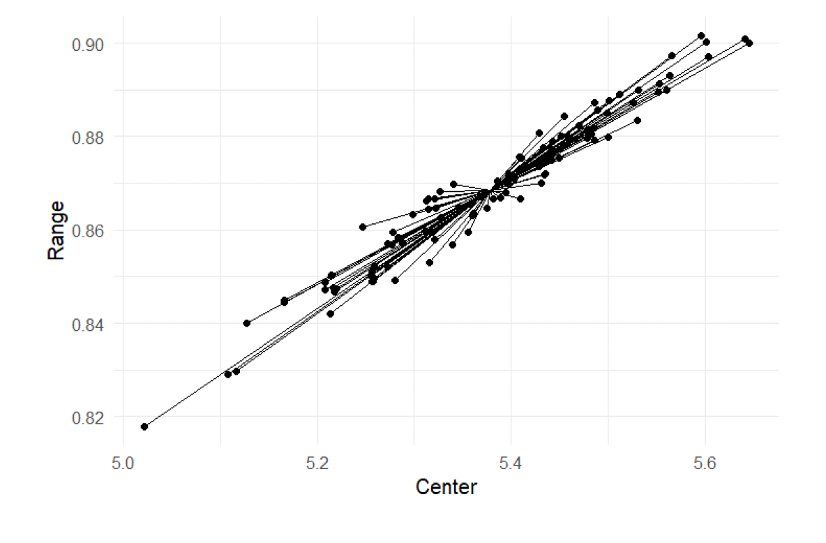
We performed this process for the remaining 99 simulated samples and populations, calculating the centers and ranges of the 95% prediction intervals. Figure 1 illustrates these centers and ranges across the 100 replications. The point from which confidence intervals originate represents the mean center and mean range of the bootstrapped samples. This point serves as the reference for comparing how each bootstrapped interval deviates from the average estimate across all samples. This range was used as a benchmark in the following subsections, when the model parameters were estimated from the same simulated data.

We now consider an actuary who used one of the three pseudo models to estimate the parameter and compute the predictions: the Poisson model with the same conditional mean function, the negative binomial model with the same conditional mean function and size parameter equal to an unknown parameter \(a\), and a normal model with the same conditional mean function and variance equal to 1. Moreover, for each pseudo model, we considered the toy case, the intermediate case, and the most realistic case, to understand the magnitude of estimation risk and model risk under each pseudo model.

3.1. Poisson pseudo model

Our first pseudo model assumes that given \({X}\), count \({Y}\) follows a Poisson distribution with the same conditional mean function. In other words, this pseudo model correctly specifies the conditional expectation but not the conditional variance. We have:

\[ f(Y|X;\lambda) = \frac{{\exp (-\lambda ){\lambda ^y}}}{{y!}}, \]

where \(\lambda = \exp (b_1+c_1 X)\). Thus for this model, the parameter is \(\theta_1=(b_1, c_1)'\), and the pseudo log-likelihood function associated with this pseudo model is:

\[\begin{aligned} \ell\left(\theta_1\right)&=-\sum_{i=1}^n \left(b_1+c_1 x_i\right) \\ & \quad +\sum_{i=1}^n Y_i\left(b_1+c_1 x_i\right) \end{aligned} . \tag{6} \]

Since the Poisson distribution belongs to the linear exponential family, and the pseudo Poisson model correctly specifies the conditional mean, we conclude from Gouriéroux, Monfort, and Trognon (1984a, 1984b) that the above pseudo maximum likelihood (PML) estimator was asymptotically consistent. That is, when the sample size \(n\) increased, the PML estimator \(\hat\theta_ 1\) converged to the true value \(\theta_0=(0.5,0.2)\). In other words, when we use the Poisson PML to estimate this Poisson pseudo model, the pseudo true value exists and coincides with the true parameter value of the true negative binomial model. For the Poisson pseudo model:

\[ {C(X, \theta_1)} ={{\sigma ^2}(X, \theta_1)} = {\exp (b_1+c_1 X)}, \]

where \(b_1,c_1\) are the parameters that must be replaced by their estimates \(\hat b_1, \hat c_1\), respectively. It should be noted that, although the estimates \(\hat{b}_1, \hat{c}_1\) are close to their theoretical values \(b_1, c_1\), they are not equal to them. In other words, the prediction \(C(X_k, \hat \theta_1)\) has finite sample bias. For instance, for the first simulated data, we obtained, \(\hat\theta_ 1=(\hat{b}_1, \hat{c}_1) = (0.509,0.199)'\), which, as expected, was close to the true value of \(\theta\). Next, we considered the problem of predicting the mean in the population.

Toy case

In this case, the \(95\%\) prediction interval is given by equation (1). For the first simulated sample and population, we obtained the following range:

\[ \frac{1}{N}\sum\limits_{k = 1}^N {Y_k} \in [5.15,5.556].\tag{7} \]

This range is much narrower than equation (5), which resulted from underestimation of the following:

• Model risk: The real conditional distribution of \(Y\) given \(X\) is overdispersed (negative binomial), whereas the pseudo model (Poisson) assumes no overdispersion.

• Estimation risk: The range in (7) does not account for the uncertainty of the parameter estimates \(\hat{b}_1, \hat{c}_1\).

Intermediate case

We calculated the forecast interval using equation(3). To calculate the contribution of the sample to the variance (second term in the square root of equation (3)), we noted that

\[\begin{align} &\left( \frac{1}{n} \sum_{i=1}^n \frac{\partial C(x_i, \hat \theta_1)}{\partial \theta_1} \right)\\ &\quad=\left( \frac{1}{n} \sum_{i=1}^n \exp(\hat{b}_1 + \hat{c}_1 x_i), \frac{1}{n} \sum_{i=1}^n x_i \exp(\hat{b}_1 + \hat{c}_1 x_i) \right)'\\ &\quad= \left( 5.259 , 34.29 \right)', \end{align}\]

where \(\theta'_1=(\hat{b}_1, \hat{c}_1)\). Subsequently,

this range is close to equation

\[\tiny{ \begin{aligned} &nI(\hat\theta_1) \\&= -n \mathbf{E}\left[ \frac{\partial}{\partial \theta'_1} \ln f(Y_i|X_i; \hat \theta_1) \cdot \frac{\partial}{\partial \theta_1} \ln f(Y_i|X_i; \hat \theta_1) \right] \\ &= n \mathbf{E} \begin{bmatrix} \frac{\partial^2}{\partial b_1^2} \left( \exp(\hat{b}_1 + \hat{c}_1 X_i) - Y_i (\hat{b}_1 + \hat{c}_1 X_i) \right) & \frac{\partial^2}{\partial b_1 \partial c_1} \left( \exp(\hat{b}_1 + \hat{c}_1 X_i) - Y_i (\hat{b}_1 + \hat{c}_1 X_i) \right) \\ * & \frac{\partial^2}{\partial c_1^2} \left( \exp(\hat{b}_1 + \hat{c}_1 X_i) - Y_i (\hat{b}_1 + \hat{c}_1 X_i) \right) \end{bmatrix} \\ &= \begin{bmatrix} n \mathbf{E}[\exp(\hat{b}_1 + \hat{c}_1 X_i)] & n \mathbf{E}[X_i \exp(\hat{b}_1 + \hat{c}_1 X_i)] \\ * & n \mathbf{E}[X_i^2 \exp(\hat{b}_1 + \hat{c}_1 X_i)] \end{bmatrix}, \end{aligned} } \]

where the symbol \(*\) indicates the symmetric off-diagonal term. This latter can be estimated by

\[ \left[ {\begin{array}{*{20}{c}} {\sum\limits_{i = 1}^n { \exp (\hat{b}_1 + \hat{c}_1 x_i)} } & {\sum\limits_{i = 1}^n { {x_i}\exp (\hat{b}_1 + \hat{c}_1 x_i)} } \\ * & {\sum\limits_{i = 1}^n { x_i^2 \exp (\hat{b}_1 + \hat{c}_1 x_i)} } \end{array}} \right]. \]

For the first simulated sample and population:

\[ \hat V({{\hat \theta }_1}) = \left[ {\begin{array}{*{20}{c}} {0.00013597}&{ -0.00001794}\\ { *}&{0.000002752} \end{array}} \right]. \]

Therefore, from equation (3), we get:

\[ \frac{1}{N}\sum\limits_{k = 1}^N {{Y_k}} \in [{\rm{5}}{\rm{.152,5}}{\rm{.554]}}. \]

This range is close to equation (7). Although this formula corrects the estimation risk, for this Poisson model, given the consistency property of the Poisson PML, the estimation error was quite small. For instance, for this simulated dataset, the Poisson parameter estimate of \(\hat{c}_1\) was \(0.199\), compared with its true value \(0.2\).

The most realistic case

From equation (4), we get:

\[ \frac{1}{N}\sum\limits_{k = 1}^N {Y_k} \in [4.917,5.79].\tag{8} \]

This range was much wider than in the toy case and quite close to the true range given in (5), because the misspecification error of the conditional variance of the pseudo model was correctly accounted for by the term \(\hat{V}[Y-C(X, \hat{\theta})]\) in equation (4), which calculated the variance of the prediction error by sample variance, rather than by the pseudo Poisson model.

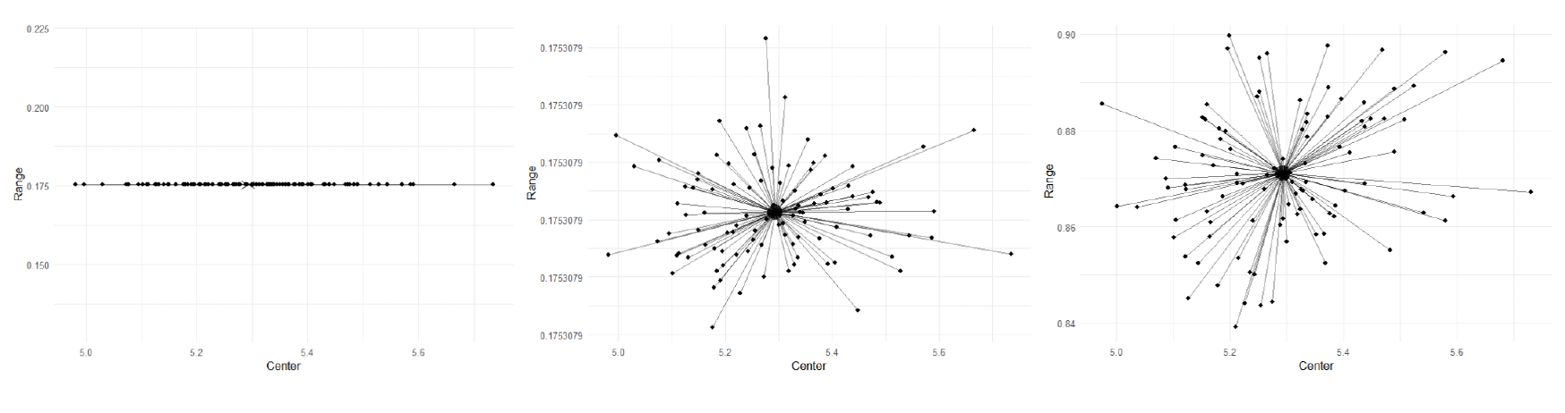
The above comparison was conducted for the same simulated sample and population. We repeated this exercise on the remaining 99 simulated samples and populations and computed the centers and ranges of the 95% prediction interval under all three cases. Figure 2 displays these centers and ranges across 100 replications.

In the left panel, the ranges and the centers are located on the same straight line. This is expected, since the range in this toy case is \(3.92\frac{1}{N}\sum_{k=1}^N \exp(\hat{b}_1+ \hat{c}_1 X_k)\), which is a multiple of the center \(\frac{1}{N}\sum_{k=1}^N \exp(\hat{b}_1+ \hat{c}_1 X_k)\). In the mid panel, the range is, on average, comparable to the range of the left panel but is more dispersed and the points are no longer located on the same straight line. Finally, the range in the right panel is, on average, much wider and comparable to Figure 1, confirming the comparison result discussed earlier for the first simulated sample and population.

3.2. Negative binomial pseudo model

Our second pseudo model assumed that, given \({X}\), response variable \({Y}\) follows a negative binomial distribution with mean \(\exp (b_2+c_2 X)\) and size parameter \(a_2\) with conditional probability mass function (PMF):

\[\small{ \begin{align} &f ( {Y}|{X}) \\ &= \left( {\begin{array}{*{20}{c}} {{Y} + \frac{1}{a_2}}\\ {{Y}} \end{array}} \right){\left( {\frac{{\exp (b_2+c_2 X)}}{{\exp (b_2+c_2 X) + \frac{1}{a_2}}}} \right)^{{y}}}{\left( {\frac{1}{{\exp (b_2+c_2 X) + \frac{1}{a_2}}}} \right)^{\frac{1}{a_2}}.} \end{align} } \]

In this model, the unknown parameter is \(\theta_2=(b_2, c_2, a_2)\). The pseudo likelihood function is:

\[\scriptsize{ \begin{align} &\ell(\theta_2)\\ &=\sum\limits_{i = 1}^n {\left\{ {{y_i}(b_2+c_2 x_i) - \left( {\frac{1}{a_2} + {y_i}} \right)\log (1 + a_2 \exp (b_2+c_2 x_i))} \right\}.} \end{align} \tag{9} } \]

Because the true DGP is also a negative binomial model, the above pseudo likelihood function is the true likelihood function^[1] and the associated MLE is asymptotically consistent. Thus, the pseudo true value associated with the maximizer of (9) exists and is once again equal to the true parameter value of the true model.^[2] For the negative binomial model:

\[ C(X, \theta_2) = \exp \left( b_2 +c_2 X \right), \]

\[ \sigma^2(X, \theta_2) =\left( \exp \left( {b}_2 + {c}_2 X \right) + \frac{\exp \left( 2{b}_2 + 2{c}_2 X \right)}{{a_2}} \right). \]

Numerically, for the first simulated sample, we get: \((\hat b_2, \hat c_2) = (0.5001,0.2013)'\) and \({\hat a_2} = 1.9816\). Next, we considered predicting the mean in the population.

Toy case

The forecast interval at \(95\%\) is given by (1). For the first simulated sample and population, we get:

\[ \frac{1}{N}\sum\limits_{k = 1}^N {Y_k} \in [4.925,5.782].\tag{10} \]

Intermediate case

Technically, the negative binomial pseudo model has three parameters: \(\theta_2=(b_2, c_2, a_2)'\). Thus, in equation 3, matrix \(\hat{V}(\theta_2)\) is of dimension \((3,3)\). Nevertheless, since \(C(x,\theta_2)=\exp(b_2+c_2 x)\) is independent of \(a_2\), we have: \(\frac{\partial}{\partial a_2}C(x, \theta_2)=0\). In other words, only the partial derivatives of \(C(x,{\theta}_2)\) with respect to \(b_2\) and \(c_2\) contribute to the square rooted term in (3), and the three-dimensional quadratic term in (3) becomes a two-dimensional matrix. We have:

\[\small{ \begin{align} &\big[ \frac{1}{n}\sum_{i=1}^n \frac{\partial C(x_i, \hat{\theta}_2)}{\partial \theta_2} \big]' \hat{V}(\theta_2) \big[ \frac{1}{n}\sum_{i=1}^n \frac{\partial C (x_i, \hat{\theta}_2)}{\partial \theta_2} \big]\\ &=\begin{bmatrix} \frac{1}{n} \sum_{i=1}^n \frac{\partial}{\partial b_2}C(x, \hat{\theta}_2) \\ \frac{1}{n} \sum_{i=1}^n \frac{\partial}{\partial c_2}C(x, \hat{\theta}_2) \end{bmatrix}' \hat{V}\begin{pmatrix}\hat b_2 \\ \hat c_2 \end{pmatrix}\begin{bmatrix} \frac{1}{n} \sum_{i=1}^n \frac{\partial}{\partial b_2}C(x, \hat{\theta}_2) \\ \frac{1}{n} \sum_{i=1}^n \frac{\partial}{\partial c_2}C(x, \hat{\theta}_2) \end{bmatrix}, \end{align}} \]

\[ \frac{1}{n} \sum_{i=1}^n \frac{\partial}{\partial b_2} C(x, \hat \theta_2) = \frac{1}{n} \sum\limits_{i = 1}^n \exp \left( \hat{b}_2 + \hat{c}_2 x_i \right) = 5.266, \]

\[ \frac{1}{n} \sum_{i=1}^n \frac{\partial}{\partial c_2} C(x,\hat \theta_2) = \frac{1}{n} \sum\limits_{i = 1}^n x_i \exp \left( \hat{b}_2 + \hat{c}_2 x_i \right) = 34.388. \]

The expression of the second term of equation (3) only involves the (2,2) submatrix of the information matrix. This submatrix can be calculated as follows:

\[ nI(\hat\theta_2) = -n\mathbf{E}\left[ \frac{\partial}{\partial \theta'_2} \ln f(Y_i|X_i; \hat \theta_2) \cdot \frac{\partial}{\partial \theta_2} \ln f(Y_i|X_i;\hat \theta_2) \cdot \right], \]

\[\tiny{ =n\mathbf{E} \begin{bmatrix} \frac{\partial^2}{\partial b^2} Y_i( b_2+ c_2 X_i) - \left( \frac{1}{a_2} + Y_i \right)\log(1 + a_2 e^{b_2+ c_2 X_i}) & \frac{\partial^2}{\partial b_2 \partial c_2} Y_i(b_2+ c_2 X_i) - \left( \frac{1}{a_2} + Y_i \right)\log(1 + a_2 e^{b_2+ c_2 X_i}) \\{*} & \frac{\partial^2}{\partial c_2^2} Y_i(b_2+ c_2 X_i) - \left( \frac{1}{a_2} + Y_i \right)\log(1 + a_2 e^{b_2+ c_2 X_i}) \end{bmatrix}, } \]

\[\small{ =\begin{bmatrix} n\mathbf{E}\left[ -\frac{(a_2 Y_i+1)\exp(b_2+ c_2 X_i)}{(a_2 \exp(b_2+ c_2 X_i)+1)^2} \right] & n\mathbf{E}\left[-\frac{X_i(a_2 Y_i+1)\exp(b_2+ c_2 X_i)}{(a_2 \exp(b_2+ c_2 X_i)+1)^2}\right] \\{*} & n\mathbf{E}\left[-\frac{X^2_i(a_2 Y_i+1)\exp(b_2+ c_2 X_i)}{(a_2 \exp(b_2+ c_2 X_i)+1)^2}\right] \end{bmatrix}.} \]

This can be estimated by

\[\small{ \begin{bmatrix} -\sum_{i=1}^{n}\frac{(a_2 y_i + 1)\exp(\hat{b}_2 + \hat{c}_2 x_i)}{(a_2 \exp(\hat{b}_2 + \hat{c}_2 x_i) + 1)^2} & -\sum_{i=1}^{n}\frac{x_i (a_2 y_i + 1)\exp(\hat{b}_2 + \hat{c}_2 x_i)}{(a_2 \exp(\hat{b}_2 + \hat{c}_2 x_i) + 1)^2} \\{*} & -\sum_{i=1}^{n}\frac{x_i^2 (a_2 y_i + 1)\exp(\hat{b}_2 + \hat{c}_2 x_i)}{(a_2 \exp(\hat{b}_2 + \hat{c}_2 x_i) + 1)^2} \end{bmatrix}.} \]

Therefore, for the second interval, we have:

\[ \frac{1}{N}\sum\limits_{k = 1}^N {{Y_k}} \in [{\rm{4}}{\rm{.928,5}}{\rm{.779]}}.\tag{11} \]

The most realistic case

The approach was exactly the same as in the most realistic case of Section 3.1. This led us to:

\[ \frac{1}{N}\sum\limits_{k = 1}^N {{Y_k}} \in [4.917,5.79].\tag{12} \]

For the negative binomial pseudo model, the three ranges (10), (11), and (12) were quite similar. This was expected because \((i)\) there is no model risk, since the pseudo model is equal to the true model of the DGP, and \((ii)\) the estimation risk is also low because of the large sample size \(n=10,000\).

Figure 3 is the analog of Figure 2 for the negative binomial pseudo model.

3.3. Normal pseudo model

We then considered a normal pseudo model with mean parameter \(\exp (b_3+c_3 X_i)\) and unit variance.^[3] Therefore,

\[ f({Y_i}|{X_i}) = \frac{1}{{\sqrt {2\pi } }}{e^{ - \frac{1}{2}({Y_i} - \exp (b_3+c_3 X_i))}}^2. \]

The parameter of this model is \(\theta_3=(b_3,c_3)'\) with:

\[ {C(X, \theta_3)} = {\exp ({\hat b_3} + {\hat c_3}{x_k})}, \quad {{\sigma ^2}(X, \theta_3)} = 1. \]

The associated log-likelihood function is, up to an additive constant:

\[ \ell(\theta_3)=- \sum\limits_{i = 1}^n {{{\left( {{y_i} - \exp (b_3+c_3 x_i)} \right)}^2}}. \]

Because the normal distribution belongs also to the linear exponential family and the pseudo model correctly specified the conditional mean, from Gouriéroux, Monfort, and Trognon (1984a, 1984b), the PML estimator is asymptotically consistent. Thus, the pseudo true value exists and is equal to the true parameter value of the true negative binomial model.

Minimizing this log-likelihood function, we obtained \(\hat \theta_3 :=(\hat b_3, \hat c_3)'=(0.521, 0.198)\) for the first simulated sample. Next, we considered predicting the mean in the population.

Toy case

In the toy case, the forecast interval at the \(95\%\) level is given by equation (1). For the simulated data, we get:

\[ \frac{1}{N}\sum\limits_{k = 1}^N {Y_k} \in [5.266,5.441].\tag{13} \]

Intermediate case

We now apply equation (3), with

\[\small{ \begin{align} \frac{1}{n}\sum\limits_{i = 1}^n {\frac{{\partial C({x_i};{{\hat \theta }_3})}}{{\partial \theta_3 '}}} &= \frac{1}{n}\sum\limits_{i = 1}^n {\frac{{\partial \exp (\hat b_3 +\hat c_3 x_i)}}{{\partial \theta_3 '}}} \\ &= \left( {\frac{1}{n}\sum\limits_{i = 1}^n {\exp (\hat b_3 +\hat c_3 x_i)}, \frac{1}{n}\sum\limits_{i = 1}^n {x_i \exp (\hat b_3 +\hat c_3 x_i)} } \right)', \end{align} } \]

where \(\theta'_3=(b_3, c_3)\), and \(\hat V({{\hat \theta }_3})\) is the estimator of \(V_{as}(\hat\theta_3)\) where,

\[\small{ \left[nI{(\theta_3 )}\right]_{h,l} = -n\mathbf{E}\left[ {\frac{\partial }{{\partial {\theta'_3}}}\ln f(Y_i|X_i;\hat \theta_3 ).\frac{\partial }{{\partial {\theta_3}}}\ln f(Y_i|X_i;\hat \theta_3 )} \right]} \]

\[\small{ = -n\mathbf{E}\left[ {\begin{array}{*{20}{c}} {\frac{{{\partial ^2}}}{{\partial b_3^2}} {{{\left( {Y_i - \exp ({b}_3 +{c}_3 X_i)} \right)}^2}} }&{\frac{\partial ^2 }{\partial {b}_3 \partial {c}_3} {{{\left( {Y_i - \exp ({b}_3 +{c}_3 X_i)} \right)}^2}} }\\ *&{\frac{{{\partial ^2}}}{{\partial c_3^2}}{{{\left( {Y_i - \exp ({b}_3 +{c}_3 X_i)} \right)}^2}} } \end{array}} \right]} \]

\[\scriptsize{ =\begin{bmatrix} -n\mathbf{E}[-2Y_i e^{{b}_3 +{c}_3 X_i} + 4X_i^2 e^{{b}_3 +{c}_3 X_i}] & -n\mathbf{E}[-2X_i Y_i e^{{b}_3 +{c}_3 X_i} + 4 X_i e^{2({b}_3 +{c}_3 X_i)}] \\ * & -n\mathbf{E}[-2Y_iX_i^2 e^{{b}_3 +{c}_3 X_i} + 4 X_i^2 e^{2({b}_3 +{c}_3 X_i)}] \end{bmatrix}.} \]

This can be estimated by

\[\scriptsize{ \begin{bmatrix} -\sum_{i=1}^{n}-2y_i e^{\hat{b}_3 +\hat{c}_3 x_i} + 4x_i^2 e^{\hat{b}_3 +\hat{c}_3 x_i} & -\sum_{i=1}^{n}-2x_i y_i e^{\hat{b}_3 +\hat{c}_3 x_i} + 4 x_i e^{2(\hat{b}_3 +\hat{c}_3 x_i)} \\ * & -\sum_{i=1}^{n}-2y_ix_i^2 e^{\hat{b}_3 +\hat{c}_3 x_i} + 4 x_i^2 e^{2(\hat{b}_3 +\hat{c}_3 x_i)} \end{bmatrix}.} \]

Therefore, for the first simulated data:

\[ \frac{1}{N}\sum\limits_{k = 1}^N {{Y_k}} \in [{\rm{5}}{\rm{.266,5}}{\rm{.441]}}.\tag{14} \]

The most realistic case

We applied equation (4), similar to the previous two sections, and obtained:

\[ \frac{1}{N}\sum\limits_{k = 1}^N {{Y_k}} \in [4.917,5.79].\tag{15} \]

Similar to the Poisson pseudo model, the range was narrowest in the toy case and widest in the most realistic case. Moreover, this latter range was quite close to the true range given in (5), highlighting that the model risk was correctly accounted for in the most realistic case.

Figure 4 is the analog of Figures 2 and 3.

4. Accounting for model risk in model comparison: Methodology

The same framework can be used to compare the performance of different models. For a given model \(j\), we define the performance measure:

\[ Perf_j(\psi):= \frac{1}{N}\sum_{k=1}^N \psi(Y_k, X_k, C_j(X_k, \hat{\theta})),\tag{16} \]

where \(C_j(X_k, \hat{\theta})\) is the prediction of \(Y_k\) given \(X_k\) under model \(j\), and \(\psi\) is a known loss function.

For the loss function \(\psi\), popular choices include the following:

• We can take \(\psi(Y_k, X_k, C(X_k, \hat{\theta}))=C(X_k, \hat{\theta})\). In this case, the performance defined in (16) is simply the prediction of \(\frac{1}{N}\sum_{k=1}^N Y_k\). For this choice of \(\psi\), the performance \(Perf_j(\psi)\) can be computed without observation of \(Y_k\), but only \(X_k\) on the population.

• A quadratic loss corresponds to \(\psi(Y_k, X_k, C(X_k, \hat{\theta}))=[Y_k-C(X_k, \hat{\theta})]^2\). For this choice of \(\psi\), we need the observation of both \(Y_k\) and \(X_k\) in the validation population. In other words, in this case, the computation of performance is similar to standard out-of-sample model validation.

• It could also be some score function, such as the log-density of \(Y_k\) given \(X_k\), if model \(j\) is likelihood based.

• If the response variable \(Y\) is count valued, we could also consider the Poisson deviance: \(\psi(Y_k, X_k, C(X_k, \hat{\theta}))\) \(=\) \(2 \{ Y_{k} \log(Y_{k}/C(X_k, \hat{\theta}))\) \(-\) \((Y_{k}-C(X_k, \hat{\theta})) \}\). For this choice of \(\psi\), we need observations for both \(Y_k\) and \(X_k\).

By considering different functions of interest \(\psi\), we studied the predictive properties of the competing pseudo models. In our simulation, we used \(\psi(X,Y;\theta)=\psi(X,Y,C(X,\theta))=(Y-C(X, \theta))^2\); therefore, we obtained the criterion of predictive accuracy.

The remainder of this section focused on how \(Perf_j(\psi)\) can be used to rank the models. In the classical model comparison approach, after a performance measure is chosen (such as AIC, BIC, or Poisson deviance), the model with the smallest performance is deemed the best model, and the remaining models are discarded. Moreover, the best model is assumed to be the correct model. This approach does not account for the impact of sampling uncertainty on performance \(Perf_j\)’s. Since both \(n\) and \(N\) are large, by applying the consistency of the estimator (on the training sample) and the law of large numbers (on the out-of-sample population), the above performance measure converges to its true value, called theoretical performance:

\[ TPerf_j(\psi)= \mathbb{E}[\psi(X, Y, C_j(X, \theta^*_{j0}))], \]

where \(\theta^*_{j0}\) is the pseudo true value of pseudo model \(j\). Clearly, a smaller \(TPerf_j\) means a better model \(j\). However, this theoretical value is not observed, but only \(Perf_j(\psi)\) is observed and can be compared across different models \(j\). Thus, when comparing different models, the uncertainty due to the unobservability of \(TPerf_j\) for different \(j\) must be accounted for. In other words, the notion of best model becomes probabilistic. GM derived statistical tests to determine whether one candidate model was superior to another at a given confidence level after accounting for sampling uncertainty.

To fix the ideas, we considered two competing models and tested the null hypothesis:

\[ \mathcal{H}_0: [TPerf_1({\psi }) = TPerf _2({\psi})]. \]

For instance, if \(\psi(Y_k, X_k, C(X_k, \hat{\theta}))=C(X_k, \hat{\theta})\), then we were testing whether the predictions of two models were indistinguishable; if \(\psi(Y_k, X_k, C(X_k, \hat{\theta}))=[Y_k-C(X_k, \hat{\theta})]^2\), then we were testing whether the two models had comparable least square prediction errors.

Since the theoretical performances \(TPerf_1({\psi }), TPerf_2({\psi })\) involved in \(\mathcal{H}_0\) are not observable, but can only be approximated by their sample counterpart, GM’s Corollary 4 derived the asymptotic distribution of the difference of these sample counterparts:

\[\begin{align} \sqrt{n}(Perf _1({\psi})&-Perf _2({\psi})) \sim \mathcal{N}(TPerf_1({\psi })\\ &-TPerf_2({\psi }), w_1^2+w_2^2),\tag{17} \end{align}\]

where

\[\scriptsize{\begin{align} &w_1^2 \\ &= \left[ {\frac{1}{{\sqrt {{\mu}} }}{\mathbf{E}_0}\left( {\frac{{\partial {{\tilde \psi }_1}}}{{\partial {{\theta '}_1}}}} \right),\frac{1}{{\sqrt {{\mu}} }}{\mathbf{E}_0}\left( {\frac{{\partial {{\tilde \psi }_2}}}{{\partial {{\theta '}_2}}}} \right)} \right]{V_{as}}\left( {\begin{array}{*{20}{c}} {{{\hat \theta }_{1}}}\\ {{{\hat \theta }_{2}}} \end{array}} \right){\left[ {\frac{1}{{\sqrt {{\mu}} }}{\mathbf{E}_0}\left( {\frac{{\partial {{\tilde \psi }_1}}}{{\partial {{\theta '}_1}}}} \right),\frac{1}{{\sqrt {{\mu}} }}{\mathbf{E}_0}\left( {\frac{{\partial {{\tilde \psi }_2}}}{{\partial {{\theta '}_2}}}} \right)} \right]^\prime }, \end{align}}\]

where \(\mathbf{E}_0\) is the expected value with respect to the real data and \({V_{as}}\left( {\begin{array}{*{20}{c}} {{{\hat \theta }_{1}}}\\ {{{\hat \theta }_{2}}} \end{array}}\right)\) is the asymptotic covariance matrix of the (rescaled) estimators \(\sqrt{n}{\hat \theta }_{1}\) and \(\sqrt{n} {\hat \theta }_{2}\), and

\[ w_2^2 = \frac{1}{{\mu } }{V_0}[{{\psi }_1}(X,Y;\theta _{10}^*) - {{ \psi }_2}(X,Y;\theta _{20}^*)]. \]

In this context, \(w_1^2\) is the contribution of estimation uncertainty of both models 1 and 2, whereas \(w_2^2\) is the contribution of sampling uncertainty for the out-of-sample population.

As a consequence of equation (17), at the 95% confidence level, the null hypothesis is rejected, if

\[ |Perf_{1}(\psi ) - Perf_{2}(\psi )| < \frac{{1.96}}{{\sqrt n }}\sqrt {\hat w_1^2 + \hat w_2^2}. \]

Moreover, where \(\mathcal{H}_0\) is rejected, we can distinguish two cases. If \(Perf_{1}{ }(\psi ) - Perf_{2}{(\psi )} > \frac{{1.96}}{{\sqrt n }}\sqrt {\hat w_1^2 + \hat w_2^2}\), then conclude that \(TPerf({\psi _1}) > TPerf({\psi _2})\); otherwise we conclude that \(TPerf({\psi _1}) < TPerf({\psi _2})\).

In practice, \(w_2^2\) can be estimated by its sample counterpart:

\[ \hat{w_2^2}= \frac{1}{{\mu } n} \sum_{i=1}^n (\psi _1(X_i,Y_i;\hat{\theta}_1) - \psi_2(X_i,Y_i;\hat{\theta}_{2})-\hat{m}_1+\hat{m}_2)^2, \]

where \(\hat{m}_1\) (respectively, \(\hat{m}_2\)) is the sample mean of \({{\psi }_1}(X_i,Y_i;\hat{\theta}_1)\) (respectively, \({\psi }_2(X_i,Y_i;\hat{\theta}_2)\)) on the training sample.

The estimation of \(w_1^2\) is more involved. It is the covariance matrix of the estimators of the two models and was not discussed by GM. The following section considered two methods, one for parametric models, based on the same type of asymptotic expansion as in GM, and one that was more general and applicable to many models, including machine learning models.

4.1. Parametric case

We first assumed that both models 1 and 2 were parametric, with fixed numbers of parameters \(\dim(\theta_1)\) and \(\dim(\theta_2)\). Moreover, we assumed that both models were estimated by maximizing their respective pseudo likelihood functions:^[4]

\[ \begin{aligned} \hat{\theta}_j&=\arg \max_{\theta_j} H_j(\theta_j)\\&= \arg \max_{\theta_j} \sum_{i=1}^n \ln f_j(Y_i|X_i, \theta_j), \\ j&=1,2, \end{aligned} \]

where \(f_1\) and \(f_2\) are the conditional PMF of \(Y\) given \(X\) under models 1 and 2, respectively. We also assumed that when \(n\) goes to infinity, \(\hat{\theta}_1\) and \(\hat{\theta}_2\) converge to their respective pseudo true values \(\theta^*_{10}\), \(\theta^*_{20}\). Then, a first-order expansion of the likelihood functions in a neighborhood of the true pseudo values leads to (see e.g., equation (3.1) of Newey and McFadden 1994):

\[\begin{align} 0 &=\frac{1}{n} \sum_{i=1}^n \nabla_{\theta_1} \ln f_1(Y_i|X_i, \theta^*_{10}) \\&\quad+ \underbrace{\Big[\frac{1}{n} \sum_{i=1}^n \nabla_{\theta_1 \theta_1} \ln f_1(Y_i|X_i, \theta_1) \Big] }_{:=M_1}( \hat{\theta}_1- \theta^*_{10}), \end{align}\tag{18}\]

\[\begin{align} 0 &=\frac{1}{n} \sum_{i=1}^n \nabla_{\theta_2} \ln f_2(Y_i|X_i, \theta^*_{20}) \\&\quad+ \underbrace{\Big[\frac{1}{n} \sum_{i=1}^n \nabla_{\theta_2 \theta_2} \ln f_2(Y_i|X_i, \theta_2) \Big]}_{:=M_2} ( \hat{\theta}_2- \theta^*_{20}), \end{align}\tag{19} \]

where \(\nabla_{\theta}\) and \(\nabla_{\theta \theta}\) are the first- and second-order differentials with respect to parameter \(\theta\), respectively. Multiplying through by \(\sqrt{n}\) and solving for \(\sqrt{n}(\hat{\theta}_1- \theta^*_{10})\) and \(\sqrt{n}( \hat{\theta}_2-\theta^*_{20})\), respectively, we have

\[ \begin{aligned} \sqrt{n}(\hat{\theta}_1- \theta^*_{10}) &=-M_1^{-1} \frac{1}{\sqrt{n}} \sum_{i=1}^n \nabla_{\theta_1} \ln f_1(Y_i|X_i, \theta^*_{10}),\\ \sqrt{n}(\hat{\theta}_2- \theta^*_{20}) &=-M_2^{-1} \frac{1}{\sqrt{n}} \sum_{i=1}^n \nabla_{\theta_2} \ln f_2(Y_i|X_i, \theta^*_{20}). \end{aligned} \]

By the law of large numbers, when \(n\) goes to infinity, the two matrices \(M_1\) and \(M_2\) converge to constant Hessian matrices:

\[\begin{align} M_1 &\longrightarrow H_1 := \mathbb{E}[\nabla_{\theta_1 \theta_1} \ln f_1(Y_i|X_i, \theta^*_{10})], \\ M_2 &\longrightarrow H_2 := \mathbb{E}[\nabla_{\theta_2 \theta_2} \ln f_2(Y_i|X_i, \theta^*_{20})], \end{align}\]

and by the central limit theorem, the \([\dim(\theta_1)+\dim(\theta_2)]-\)dimensional joint distribution of

\[\small{ \Big(\frac{1}{\sqrt{n}} \sum_{i=1}^n \nabla_{\theta_1} \ln f_1(Y_i|X_i, \theta^*_{10}), \frac{1}{\sqrt{n}} \sum_{i=1}^n \nabla_{\theta_2} \ln f_2(Y_i|X_i, \theta^*_{20})\Big)', } \]

converges to a multivariate normal distribution with zero mean vector and block covariance matrix:

\[ \begin{aligned} J:=\begin{bmatrix} J_{11} & J_{12} \\ J'_{12} & J_{22} \end{bmatrix}, \end{aligned} \]

where \(J_{ij}\) is of dimension \(\dim(\theta_i) \times \dim(\theta_j)\) for \(i,j=1,2\), and is given by:

\[ \begin{aligned} J_{11}&=\mathbb{E}[\nabla_{\theta_1} \ln f_1(Y_i|X_i, \theta^*_{10}) \nabla_{\theta_1} \ln f_1(Y_i|X_i, \theta^*_{10})'], \\ J_{12}&=\mathbb{E}[\nabla_{\theta_1} \ln f_1(Y_i|X_i, \theta^*_{10}) \nabla_{\theta_2} \ln f_2(Y_i|X_i, \theta^*_{20})'],\\ J_{22}&=\mathbb{E}[\nabla_{\theta_2} \ln f_2(Y_i|X_i, \theta^*_{20}) \nabla_{\theta_2} \ln f_2(Y_i|X_i, \theta^*_{20})']. \end{aligned} \]

In other words, J is the joint information matrix, and the two diagonal blocks \(J_{11}\) and \(J_{22}\) are the information matrix associated with models 1 and 2, respectively.

Since the limits of \(M_1\) and \(M_2\), (i.e., matrices \(H_1, H_2\)) are deterministic, we applied the Slutsky’s lemma and concluded that the joint distribution of \(\sqrt{n}\Big(\hat{\theta}_1- \theta^*_{10}, \hat{\theta}_2- \theta^*_{20}\Big)\) converges to the block product matrix:

\[\scriptsize{ \begin{align} \begin{bmatrix} H_1^{-1} J_{11} H_1^{-1} & H_1^{-1} J_{12} H_2^{-1} \\ H_2^{-1} J_{21} H_1^{-1} & H_2^{-1} J_{22} H_2^{-1} \end{bmatrix}&= \begin{bmatrix} J_{11}^{-1} & H_1^{-1} J_{12} H_2^{-1} \\ H_2^{-1} J_{21} H_1^{-1} & J_{22}^{-1} \end{bmatrix}\\&:={V_{as}}\left( {\begin{array}{*{20}{c}} {{{\hat \theta }_{1}}}\\ {{{\hat \theta }_{2}}} \end{array}} \right), \end{align}\tag{20} } \]

where we used the usual relationship between the Hessian matrix and the information matrix:

\[ H_1 =-J_{11} , H_2 =-J_{22}. \]

By replacing matrices \(J_{i,j}\) with their sample counterparts, we get an estimate of \(w_1^2\) in equation (17).

4.2. General case

A downside of equation (17) is that the definition of \(w_1^2\) assumes implicitly that the dimension of the parameter is fixed. This holds true for parametric models, but it is no longer the case for machine learning models, whose number of parameters could be random and/or increasing in \(n\). Many machine learning models are estimated using non-likelihood based methods (such as those based on cross-validation) and involve regularization hyperparameters. Moreover, many such methods, such as neural networks, involve a much larger number of parameters, and the associated objective function could be highly nonconvex. Consequently, the fitted parameters need not necessarily satisfy the first-order expansions (18) and (19).

Consequently, we can no longer rely on standard asymptotic expansion (17) to get the distribution of \(\sqrt{n}(Perf_1({\psi })-Perf_2({\psi }))\). Nevertheless, it is still possible to approximate this distribution through bootstrapping. We generated \(100\) new training databases of size \(n\) by simulating with replacement from the original training database. Similarly, we created \(100\) new validation populations of size \(N\) by simulating with replacement from the original population. Then we estimated both models 1 and 2 from these \(100\) simulated training databases and computed their performance measures \(Perf_1(\psi)\) and \(Perf_2(\psi)\) on the simulated validation population to get 100 observations of \((Perf_1(\psi),Perf_2(\psi))\). Since these observations are i.i.d., by the central limit theorem, this distribution is approximately normal, with mean \((TPerf_1(\psi), TPerf_2(\psi))\). We denoted by \(\overline{m}\) and \(\hat{\sigma}\) the sample mean and standard deviation, respectively, of these observations of \(Perf_1(\psi)-Perf_2(\psi)\). Then we accepted the null hypothesis that \(TPerf_1(\psi)= TPerf_2(\psi)\), only if:

\[ \mid \overline{m} \mid < \frac{{1.96}}{\sqrt {100 }}\hat{\sigma} . \]

Clearly, in this general case, the test is computationally much more intensive than in the parametric case of Section 4.1, but it is also more straightforward to implement and more general.

5. Accounting for model risk in model comparison: Illustration using simulated data

In this section, we used simulated validation to compute, for the \(j\)-th pseudo model, its performance

\[ Per{f_{j,N}} = \frac{1}{N}\sum\limits_{k = 1}^N {\psi ({X_k},{Y_k},{C_j}({X_k},{{\hat \theta }_{j}}))}, \]

where parameter \({\hat \theta }_{j}\) is estimated from the simulation training sample.

We take

\[ {C_j}({X_k},{{\hat \theta }_{j}}) = {\mathbf{E}_j}({Y_k}|{X_k}), \]

and

\[\begin{align} \psi ({X_k},{\rm{ }}{Y_k},{\rm{ }}{C_j}({X_k},{\rm{ }}{{\hat \theta }_{j}})){\rm{ }} &= {\rm{ }}{({Y_k} - {C_j}({X_k},{\rm{ }}{{\hat \theta }_{j}}))^2}\\&:= \psi (X_k, Y_k, \hat{\theta}_j), \end{align} \]

where \({\mathbf{E}_j}\) is the expected value with respect to the \(j\)-th pseudo model. We denoted by \(\hat{\theta}_1\), \(\hat{\theta}_2\), and \(\hat{\theta}_3\) the estimator for the Poisson, negative binomial, and normal pseudo models, respectively.

5.1. Parametric case

For the parametric case,

\[\begin{align} Per{f_{j,N}}(\psi )&= \frac{1}{N}\sum\limits_{k = 1}^N [Y_{k}-\exp (\hat{b}_i+\hat{c}_i X_k)]^2,\\ j&=1,2,3. \end{align} \]

We obtained \(Per_{1,N}(\psi) = 25.993\) for the Poisson model, \(Per_{2,N}(\psi) = 25.9954\) for the negative binomial model, and \(Per_{3,N}(\psi) = 25.9949\) for the normal model using the same simulated sample and population described in Section 3. It is worth noting that the negative binomial pseudo model appeared to perform worse than expected, which can be attributed to random perturbations in the generated responses. It is important to know that this result was specific to this sample; in other simulated samples, the performance ranking may differ.

Therefore,

\[\begin{align} \mathbf{E}_0\left( \frac{\partial {\psi}_j}{\partial \theta'} \right)&=\mathbf{E}_0 \left[ e^{b_j+c_j X_i}(Y_i-e^{b_j+c_j X_i}) \begin{pmatrix} -2 \\ -2X_i \end{pmatrix} \right]', \\ \forall j&=1,2,3, \end{align} \]

where \(\mathbf{E}_0\) is the expected value with respect to true distribution of \((X,Y)\) which is negative binomial. The above expression can be estimated by replacing \(b_j,c_j\) with their estimates \(\hat{b}_j,\hat{c}_j\), and the expectation by its sample average. We obtained \((0.0056, 0.1452)\) for the Poisson model, \((-0.0322,-0.218)\) for the negative binomial model, and \((0.0068,0.0518)\) for the normal model.

As an illustration, we compared the pseudo Poisson and pseudo normal models with PMFs:

\[\begin{align} f_{1}(Y|X_i,\theta_{1})&=\frac{e^{-\lambda} \lambda^{y}}{y!}, \\ \lambda&=\exp(b_1+c_1{X_i}),\tag{21} \end{align}\]

\[\begin{align} f_{3}(y|X_i,\theta_{3})&=\frac{1}{\sqrt{2\pi}}e^{-\frac{1}{2}(y-\mu)^2},\\ \mu&=\exp(b_3+c_3{X_i}), \end{align}\tag{22} \]

and deduced that:

\[ \nabla_{\theta_1} \ln f_1(Y_i; X_i, \theta_1) =(Y_i-e^{b_1+c_1X_i}) \begin{pmatrix} 1 \\ X_i \end{pmatrix} , \]

\[ \nabla_{\theta_3} \ln f_1(Y_i; X_i, \theta_3) =(Y_i-e^{b_3+c_3 X_i})e^{b_3+c_3 X_i} \begin{pmatrix} 1 \\ X_i \end{pmatrix}. \]

Therefore,

\[ J_{11}=E\begin{bmatrix} (Y_i-e^{b_1+c_1 X_i})^2\begin{pmatrix} 1 & X_i \\ X_i & X_i^2 \end{pmatrix} \end{bmatrix},\tag{23} \]

\[\scriptsize{ J_{12}=E\begin{bmatrix} (Y_i-e^{b_1+c_1 X_i}) (Y_i-e^{b_3+c_3 X_i}) e^{b_3+c_3 X_i} \begin{pmatrix} 1 & X_i \\ X_i & X_i^2 \end{pmatrix} \end{bmatrix},\tag{24}} \]

\[ J_{22}=E\begin{bmatrix} (Y_i-e^{b_3+c_3 X_i})^2 e^{2b_3+2c_3 X_i}\begin{pmatrix} 1 & X_i \\ X_i & X_i^2 \end{pmatrix} \end{bmatrix}.\tag{25} \]

Thus, by equation (20), for the first simulated data we obtained,

\[\small{ \begin{align} {V_{as}}\left( {\begin{array}{*{20}{c}} {{{\hat \theta }_{1}}}\\ {{{\hat \theta }_{3}}} \end{array}} \right)&= \begin{bmatrix} J_{11}^{-1} & H_1^{-1} J_{12} H_2^{-1} \\ H_2^{-1} J_{21} H_1^{-1} & J_{22}^{-1} \end{bmatrix}\\ &= \begin{bmatrix} 0.499 & -0.062 & 0.410 & -0.051 \\ * & 0.008 & -0.051 & 0.007 \\ * & * & 0.0264 & -0.003 \\ * & * & * & 0.0003 \end{bmatrix}. \end{align} } \]

Thus

\[\scriptsize{ \begin{align} &w_1^2 \\ &= \left[ {\frac{1}{{\sqrt {{\mu}} }}\mathbf{E_0}\left( {\frac{{\partial {{ \psi }_1}}}{{\partial {{\theta '}_1}}}} \right),\frac{1}{{\sqrt {{\mu}} }}\mathbf{E_0}\left( {\frac{{\partial {{ \psi }_3}}}{{\partial {{\theta '}_3}}}} \right)} \right]{V_{as}}\left( {\begin{array}{*{20}{c}} {{{\hat \theta }_{1}}}\\ {{{\hat \theta }_{3}}} \end{array}} \right){\left[ {\frac{1}{{\sqrt {{\mu}} }}\mathbf{E_0}\left( {\frac{{\partial {{ \psi }_1}}}{{\partial {{\theta '}_1}}}} \right),\frac{1}{{\sqrt {{\mu}} }}\mathbf{E_0}\left( {\frac{{\partial {{ \psi }_3}}}{{\partial {{\theta '}_3}}}} \right)} \right]^\prime }\\ &=0.002017, \end{align} } \]

\[\begin{align} w_2^2 &= \frac{1}{{\mu } }{V_0}[{{\psi }_1}(X,Y;\theta_1) - {{ \psi }_3}(X,Y;\theta _3)]\\&=0.000244, \end{align} \]

where \({V_0}\big[{{\tilde \psi }_1}(X,Y;\theta _1) - {{\tilde \psi }_3}(X,Y;\theta _3)\big]\) is the sample of variance of the difference of loss functions of pseudo Poisson and pseudo normal.

Therefore, \(Perf_{1}(\psi ) - Perf_{3}{(\psi )} < \frac{{1.96}}{{\sqrt n }}\sqrt {\hat w_1^2 + \hat w_2^2}\), and we concluded that \(TPerf({\psi _1}) < TPerf({\psi _3})\). In other words, the Poisson pseudo model provided a significantly more accurate prediction. How should we interpret this result? Does it align with both pseudo models showed \(C(X,\theta_j) = \exp(b_j + c_j X)\) for \(j=1,3\), and that both PML estimators were asymptotically consistent? In fact, the superiority of the Poisson pseudo model reflects that the Poisson PML has smaller asymptotic variance than the normal PML, since the Poisson model is more similar to the true negative binomial model than the normal model.

The resulting \(p=6.45 \times 10^{-5}\) indicates that the difference in performance was highly statistically significant.

5.2. General case

Using the bootstrap method, we simulated 100 new data by replacement and obtained 100 observations of \((Perf_1(\psi),Perf_3(\psi))\), where the first model was pseudo Poisson and the second was pseudo normal. The distribution of \(\sqrt N (Perf_1(\psi)-Perf_3(\psi))\) is approximately normal with mean \((TPerf_1(\psi),TPerf_3(\psi))\). Using the bootstrap data, we found:

\[ \overline{m}=-0.00512, \hat\sigma=0.00642. \]

Consequently, since

\[ \mid \overline{m} \mid > \frac{{1.96}}{\sqrt {100 }}\hat{\sigma} , \]

we rejected the null hypothesis that \(TPerf_1(\psi)=TPerf_3 (\psi)\), indicating a statistically significant difference between the two performance measures. The \(p-\)value \(=1.332268 \times 10^{-15}\). Thus, in this specific example, both methods led to the same conclusion.

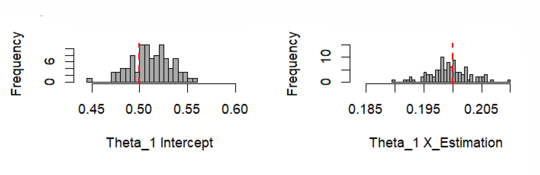
Figure 6 displays the histograms of the estimated parameters, and the graph in Figure 7 demonstrates the performance differences for the pseudo Poisson, pseudo negative binomial, and pseudo normal models. In Figure 6, parameters \(\hat{\theta}_1\) and \(\hat{\theta}_2\) were estimated from bootstrap samples, with each subplot showing the distribution of the intercept and predictor variable \(X_i\). The consistent central tendency and reasonable spread suggest reliable parameter estimation. Figure 7 shows a histogram of performance differences, with the \(x\)-axis representing the difference and the \(y\)-axis representing the probability. The symmetrical distribution around the mean indicates that the performance differences follow a normal distribution.

In addition to the three parametric pseudo models, we included an XGBoost model, which has gained popularity in actuarial science (Henckaerts et al. 2021; Kiermayer 2022; So 2024). XGBoost is a machine learning method that uses gradient boosting, which sequentially improves the model by combining predictions from multiple decision trees, where each tree aims to correct the errors made by the previous tree. The trees are trained by minimizing an objective function containing two parts, the training loss and the regularization term that controls the tree structure.

\[ L(\theta) + \Omega(\theta),\tag{26} \]

where \(L(\theta)\) is the negative Poisson pseudo likelihood function (up to a constant)

\[ L(\theta)= - \sum_{i=1}^{n} \left( y_i \cdot \log(\hat{y}_i) - \hat{y}_i \right), \]

where \(y_i\) represents the observed value, \(\hat{y}_i = \exp(\theta' \mathbf{X_i})\) denotes the value predicted by the model, with \(\mathbf{X_i}\) being the vector of variables and \(\theta\) representing the model’s parameters. The second, regularization term penalizes the complexity of the model through

\[ \Omega(\theta) = \gamma T + \frac{1}{2} \lambda \sum_{j=1}^{T} w_j^2, \]

where \(T\) is the number of leaves in the tree, \(w_j^2\)’s are the weights of the leaves that can be optimally obtained by \(w_j^*=\frac{G_j}{H_j+\lambda}\), \(\gamma\) controls the number of leaves, and \(\lambda\) is the \(L^2\) regularization term. XGBoost optimizes the objective function using gradient descent. When growing a tree, XGBoost evaluates the quality of a split based on the gain, which measures the improvement in the objective function:

\[\small{\begin{align} \frac{1}{2} \left[ (H_L + \lambda G_L^2) + (H_R + \lambda G_R^2) - (H_L + H_R + \lambda (G_L + G_R)^2) \right] - \gamma, \end{align}} \]

where \(G_L\) and \(G_R\) are the sums of the gradients for the left and right splits, and \(H_L\) and \(H_R\) are the sums of the second-order gradients.

While the model estimation is derived from the sample, comparisons are made across the population. The mean squared error (MSE) was chosen as the metric to compare model performance because it provides a clear measure of prediction accuracy.

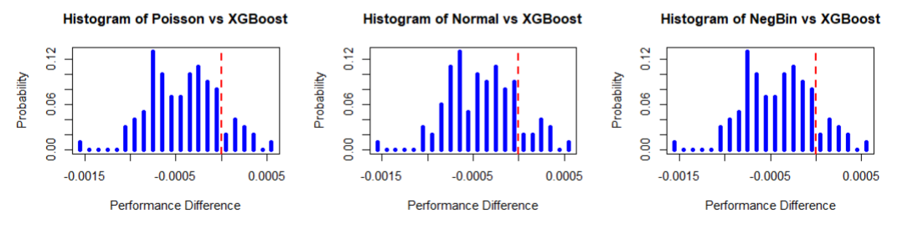
Using the XGBoost package in R, we set the objective function to be Poisson and the evaluation metric to be rmse. We set the model parameters as follows: \(\gamma = 0\), \(\lambda = 1\), and \(\eta = 0.1\). We trained the model over 100 boosting rounds, actively monitoring its performance on the validation set. From each of the 100 simulated samples and populations (which we called primary simulation), we simulated 100 bootstrapped samples and populations, trained the four candidate models on these bootstrapped samples, and computed each model’s performance on bootstrapped populations. We then plotted a histogram of the 100 performance differences between the models, obtained from these 100 primary simulations.

The three histograms in Figure 8 demonstrate that the performance differences between three pseudo models and XGBoost follow an approximately normal distribution. The three parametric models are better than XGBoost, since the sample mean of the performance is less than 0. Table 1 illustrates the comparison test mentioned in Section 4.2.

Table 1 represents the analysis using MSE as the performance measure. The results indicate that the negative binomial model consistently outperformed the other models. The Poisson model also exhibited strong performance, outperforming the normal and XGBoost models. This was expected, since the true model is negative binomial, and is far from the tree-based model that underlies the XGBoost model.

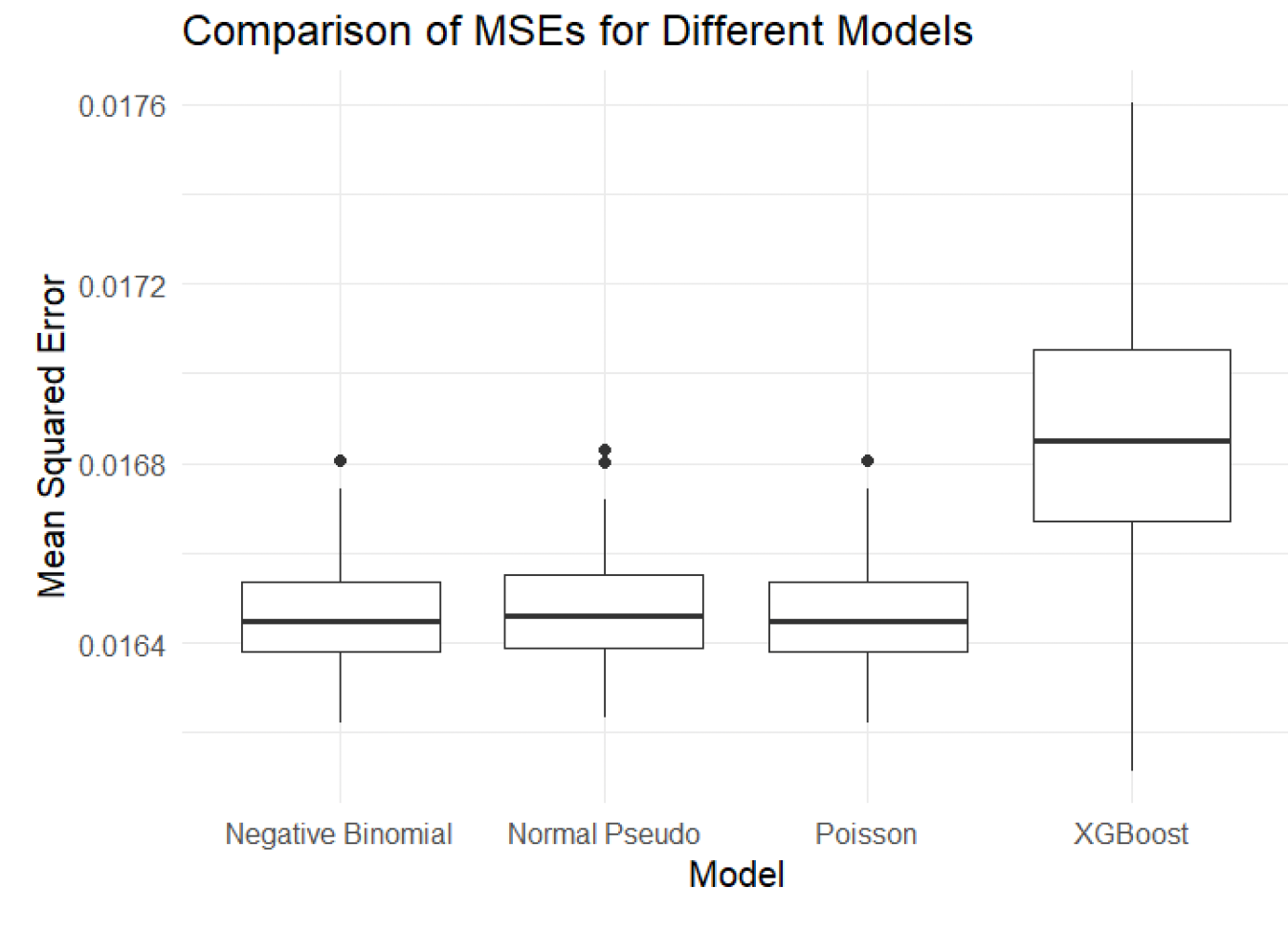
Similarly, the boxplot in Figure 9 shows the MSE comparisons across the models. The negative binomial pseudo model, which aligns with the distribution of the simulated real data, served as a benchmark for comparison. XGBoost exhibited the highest MSE, indicating lower prediction accuracy. Moreover, both the pseudo Poisson and the pseudo normal models were asymptotically unbiased.

The analyses in this section were conducted using MSE as the performance measure. The Appendix provides the analog of Figure 9, where Poisson deviance was used as an alternative performance measure.^[5]

6. Real data application

6.1. Data description

We used the fremotor3freq9907b dataset, provided in the R package CAS (see Charpentier 2014), which comprises various attributes of one-year motor insurance policies. The dataset included the following variables:

• IDpol: policy identification number

• Year: year when the policy was active, ranging from 2002 to 2007

• NbClaim: number of claims reported under the policy (the response variable)

• Expo: exposure, representing the number of years the policy was in force

• Usage: categorical variable describing vehicle use (e.g., private, commercial)

• VehType: type of vehicle insured (e.g., sedan, SUV)

• VehPower: vehicle power categorized into classes

The dataset was randomly split, with 70% of the data allocated for model training and the remaining 30% reserved for validation.

6.2. Prediction using different models

We employed three pseudo models, Poisson, negative binomial, and XGBoost. We calculated confidence intervals under the most realistic case:

• For the Poisson model \[\frac{1}{N}\sum_{k=1}^N Y_k \in [0.154, 0.167].\]

• For the negative binomial model \[\frac{1}{N}\sum_{k=1}^N Y_k \in [0.158, 0.165].\]

• For the XGBooost method \[\frac{1}{N}\sum_{k=1}^N Y_k \in [0.159, 0.165].\]

Thus the three candidate models provided similar average prediction and range for the entire portfolio. However, it is possible that one of the three models dominated the other two on individual risks segmentation. That is, the two other models might have wrongly predicted high risks for some policies and wrongly predicted lower risks for others, with both effects partially canceling out throughout the entire portfolio. In this case, these two models could put the insurer at a disadvantage compared with its competitors. To see whether this is the case, we applied the methodology from Section \(4\) to formally compare the three candidate models.

6.3. Model performance comparison

The models’ performance on real datasets was compared using the MSE of their predictions. We bootstrapped this database 100 times and obtained 100 simulated samples and 100 simulated populations. We calculated the MSEs based on the out-of-sample predictions.

The boxplot in Figure 10 illustrates that the negative binomial model exhibited a broader range of MSE values, which suggests variability in performance, possibly influenced by different data subsets.^[6] In contrast, the XGBoost model demonstrated a lower MSE, indicated by a lower positioned point and a significantly shorter error bar, reflecting higher consistency and reliability in predictions across various scenarios. The boxplot indicates that the XGBoost model performed better compared with the negative binomial model. Recall that in Section 5, where the DGP was negative binomial, and the other parametric pseudo models (Poisson and normal) were deliberately chosen to have correct specification of the mean, the XGBoost method did not have an advantage. However, in this section, where true DGP is unknown and the competition is more fair, XGBoost was the best model. This example confirms the widely reported usefulness of machine learning methods for real insurance data.

Using the bootstrap method, we obtained 100 observations of \((Perf_1(\psi),Perf_2(\psi))\) where \(TPerf_1(\psi), TPerf_2 (\psi)\) represent the theoretical performance of the negative binomial and XGBoost methods, respectively, and \(Per{f_{j,N}}(\psi )= \frac{1}{N}\sum\limits_{k = 1}^N [Y_{k}-\exp (\hat{b}_i+\hat{c}_i X_k)]^2\). The distribution of \(\sqrt N (Perf_1(\psi)-Perf_2(\psi))\) is approximately normal with mean \((TPerf_1(\psi),TPerf_2(\psi))\). We obtained

\[ \overline{m}=0.00999, \hat\sigma=0.000145. \]

As \(|\overline{m}| > \frac{1.96}{\sqrt{100}} \hat{\sigma}\), we rejected the null hypothesis that \(TPerf_1(\psi) = TPerf_2(\psi)\). Therefore, \(TPerf_1(\psi) < TPerf_2(\psi)\), indicating that the pseudo XGBoost model performed better than the pseudo negative binomial model.

7. Conclusion

This study adapted the methodology of Gouriéroux and Monfort (2021) and applied it to property and casualty insurance data to properly quantify model risk for both prediction and model selection. For prediction, this method allowed us to account for both bias and uncertainty related to potential misspecifications. The most important message concerning prediction is that traditional approaches, such as the toy case and the intermediate case, underestimate the uncertainty introduced by model risk. For model selection, the proposed method allowed us to compare whether the average premium given by one model was significantly higher than that of competing models, and to compare the goodness of fit of different models. An important point concerning model selection is that, after accounting for model risk, the hierarchy between different models becomes probabilistic.

The framework investigated in this study is only a starting point toward systematic treatment of model risk. For instance, a key assumption that the proposed analysis adopts throughout the paper is that \((Y,X)\) is i.i.d. across both the sample and the population. An interesting extension would be to investigate how macro-level dependence can be introduced to account for systemic risk related to, say, natural disasters. Moreover, the formulas we applied were based on the central limit theorem, which might not sufficiently approximate the tail of the distribution. In other words, higher order expansions could be useful or necessary for quantifying the impact of model risk on tail risk measures such as value at risk and expected shortfall. These topics are beyond the scope of this study and are left for future research.