Applications of Gaussian-Inverse Wishart Process Regression Models in Claims Reserving

undefined

1. Introduction

The estimation of unpaid loss liabilities is one of the core tasks performed by actuaries. Such liabilities represent one of the main items on the balance sheet of a general insurer, and their estimation is critical for insurers to properly conduct business (Actuarial Standards Board 2007).

In this respect, a probabilistic estimation of these liabilities, also known as stochastic claims reserving, has gained traction in recent years, both from an internal management perspective and as a regulatory requirement imposed by authorities in many jurisdictions, to enhance the risk management practice of property and casualty insurers (Committee on Property and Liability Financial Reporting 2018).

In this paper we intend to show how Gaussian process regression (GPR) can be used as a tool to model the uncertainty surrounding the estimation of unpaid loss liabilities and that it represents a viable machine learning alternative to well-known and well-established methods in the context of claims reserving.

GPR indicates a set of powerful nonparametric, Bayesian regression and classification techniques that enable us to make probabilistic predictions incorporating prior knowledge into the modeling process. The actuarial literature provides many models for framing the point prediction of the reserve in a stochastic framework (Mack 1994; England and Verrall 2002). Nonetheless, the majority of the research relates to approaches that pertain to the frequentist field of statistics, while the adoption of Bayesian techniques is something still in its infancy (Meyers 2015).

2. Literature review

Bayesian tools are not something new in the context of claims reserving, and their first proto-application can be traced back to Bornhuetter and Ferguson (1972). Those authors show a method of estimating reserves by combining prior domain knowledge and subsequently updating it based on actual experience. The procedure—how it is presented—is not Bayesian in nature, but it contains interesting insights pointing in that direction.

The incorporation of real Bayesian techniques into the actuarial toolkit, despite their being widely known to statistician and actuarial researchers, has always been difficult due to the unavailability of mathematically tractable forms for the posterior distributions. Nonetheless, with the decreasing cost of computational power and the easier availability of Markov chain Monte Carlo (MCMC) samplers in more recent years, many interesting articles have been published demonstrating how to obtain Bayesian predictive distributions of claim liabilities.

The first appearance is to be credited to Ntzoufras and Dellaportas (2002), who used MCMC methods to obtain the prediction of the amount of outstanding automobile claims that an insurance company will pay in the near future. Remarkable is the result of Gisler and Wuethrich (2008), who showed how to obtain a closed formula for the posterior distribution of chain ladder parameters under a gamma-distributed prior. Another milestone result can be found in Meyers (2015), where the author applies MCMC sampling techniques to obtain the predictive distribution of claims reserves.

Nevertheless, approaching the claims reserving problem in a GPR framework is still a new approach, and the only relevant works are those by Lally and Hartman (2018) and Ludkovski and Zail (2021). Whereas Lally and Hartman show how it is possible to make a probabilistic projection of the claims reserve by reimagining the run-off triangle in the context of spatial statistics, the latter authors develop a similar framework introducing premium amounts and then approaching the problem by the point of view of loss ratio (LR) rather than claim amounts.

In this paper, we build on the two above-mentioned papers and generalize a claims reserving approach based on GPR. We conduct here a more extensive work on the priors. We elicit an inverse Wishart prior distribution (in Bayesian analysis, the inverse Wishart distribution is often used as a prior for the variance-covariance parameter matrix [Gelman et al. 2014]) over the covariance function of the GPR, an approach that has not been explored in the realm of actuarial science and is found only in Wilson and Ghahramani (2012) on a financial time series forecast exercise.

We test this novel GPR approach on several covariance functions, also exploring combinations of such functions. Following Lally and Hartman (2018), we re-propose the application of input warping and quantify its impact. To ensure the statistical robustness of the results, we test this approach on more than 20 different run-off triangles, with incremental amounts and LR triangles, where on each triangle and for each quantity, we conduct a grid search procedure to determine the best combination between the covariance function shape and prior parameters.

This procedure follows a traditional hyperparameter tuning process, common in many modeling routines in the context of machine learning parameter optimization. Prior articles on the topic do not include a formal procedure to identify suitable prior distributions, a common fear among those who were trained as frequentists but are now entering the Bayesian world; we hope that the proposed process will encourage more widespread adoption.

The paper is aimed at actuarial practitioners, giving a practical explanation together with examples on how to implement and experiment with the model. We provide full details about the rationales behind our choices, and we present a fully replicable routine to determine the best prior distributions. All the code to replicate and experiment with the procedure is made available in a public repository. Our ultimate goal is to generalize a claims reserving methodology based on GPR and to extend its formulation to include uncertainty estimates around loss development factors, expanding the stream of research on loss growth curves (Clark 2003; De Virgilis 2020).

3. Bayesian statistics

Bayesian statistics is a powerful branch of statistics alternative to the frequentist one. The differences between frequentist and Bayesian statistics arise fundamentally from a different philosophical “stance” toward probability. In the frequentist view, the probability of an event is defined as the limit of its relative frequency as the number of trials grows to infinity—i.e., the long-run frequency of occurrence of the event. By contrast, in Bayesian statistics, probabilities are subjective quantities that express a degree of belief in an event occurring based on the information available. These philosophical differences substantiate in a different approach to statistical modeling, especially with respect to statistical inference.

Basically, frequentist inference considers model parameters as unknown values to be estimated, with the aid of different techniques, from the observed data. By contrast, Bayesians consider them as uncertain quantities, which could vary randomly, and for which we are allowed to have a prior belief. Here lies the key concept supporting the entire Bayesian framework: inference is performed by “applying” evidence to a set of prior beliefs, resulting in a posterior belief. The analytical tool to perform this update is the Bayes rule, which is essentially a restatement of conditional probability:

$$P(A | B) = \frac{P(B | A) P(A)}{P(B)},$$

$$P(A | B) \propto P(B | A) P(A).$$

From this formula one can see how the approach is inherently probabilistic and that it generates a full range of values for the target parameters of our estimate. Unfortunately, whereas such an approach is conceptually simple, it is very hard to apply in practice, as an analytically tractable form for the posterior distribution is an exception rather than the norm. Luckily, the mathematical complexity can be dodged by adopting the so-called MCMC class of algorithms that can be used to obtain a sample of the posterior distribution, thus allowing an empirical estimation of the posterior distribution and opening a range of new possibilities in the application of Bayesian statistics (Van Ravenzwaaij, Cassey, and Brown 2018).

4. Theoretical background

As mentioned, GPR is a supervised learning technique, i.e., a regression/classification technique that fits a function on a set of training data with a known target variable. The main peculiarity, though, is that instead of fitting one function, it returns a probability distribution of all functions that can fit the observed data. Given a set of data points, there are infinitely many functions that can fit the data, and GPRs are capable of describing all these functions, assigning a probability to each one. This allows us a degree of confidence in the results of the fit. Furthermore, it allows us to incorporate prior and external knowledge into the modeling process.

The intuition behind GPRs can be difficult to grasp at first glance. Therefore, before more deeply investigating GPR details, it is worthwhile to outline the technique’s mathematical underpinnings. GPRs can be used for both classification and regression; both the subsequent theoretical paragraphs and the worked application pertain to the regression setting rather than the classification counterpart.

4.1. Distributions of functions and Gaussian processes

Before introducing GPR, we have to take a step back and introduce what Gaussian processes are. A simplified definition is that Gaussian processes are a generalization of the multivariate normal random variable. Analytically, a Gaussian process is a stochastic process (i.e., a collection of indexed random variables), $\{X_k; k \in K\}$, where, for every finite set of indices $k_1,\dots,k_n$ in the index set $K$, $\mathbf{X}_{k_1,\dots,k_n} = (X_{t_1},\dots,X_{t_k})$ is a multivariate Gaussian random variable. A 2-D Gaussian random variable, for example, is defined as

$$\begin{bmatrix} x_{1} \\ x_{2} \\ \end{bmatrix} \sim N \Bigg( \begin{bmatrix} \mu_{1} \\ \mu_{2} \\ \end{bmatrix} , \begin{bmatrix} \sigma^2_{1} \quad \sigma_{1,2}\\ \sigma_{2,1} \quad \sigma^2_{2}\\ \end{bmatrix} \Bigg)=N(\mu, \Sigma),$$

where $\mu$ represents the vector of the means of the Gaussian random variables and $\Sigma$ is the variance-covariance matrix.

Gaussian processes generalize the multivariate normal to the extent that we no longer have a vector of means and a variance-covariance matrix. Instead we have a mean function, $\mu(x)$, and a covariance function, $\Sigma(x)$, (also called a kernel) that will characterize a process with specific location and variability features. Intuitively, we can think of the covariance function as the function that fully determines the variance-covariance matrix of a multivariate normal random variable on its support.

Another very important point is that, in practical applications, the observations are always standardized and the mean function is assumed to be equal to zero (Rasmussen and Williams 2005). Therefore, the process is entirely defined by the covariance function. Here lies one of the Bayesian intuitions behind the method: a specific choice of kernel can be used to conveniently describe the prior modeler’s belief about the data. The choice of an appropriate kernel is based on assumptions such as smoothness and particular patterns to be expected in the data.

More formally, in a univariate case, we have

$$y = f(x) + \epsilon,$$

where

$$f(x) \sim GP\big( \mu(x), \Sigma(x,x') \big), \ \ \ \ \ \ \epsilon \sim N(0, \sigma^2_\epsilon),$$

where $\mu(x)$ is the mean function and the kernel $\Sigma(x,x')$ is a positive definite matrix.

Thinking about the multivariate normal, the variance-covariance matrix contains information about how univariate random variables move together. Still, with a bivariate case in mind, the covariance function specifies the variance-covariance matrix for each and every pair on the support of the univariate random variable. It is a function that will determine the variability of the functions that will fit the data.

Given this, one of the most common implementations is that of covariance functions thought of as distance functions. Loosely speaking, we can assume that the correlation between two points decays with the distance between the points. This means that closer points are expected to behave more similarly than points that are further away from each other, i.e., the function will return a value close to 1 if the two input points, $x$ and $x'$, are relatively close and a value close to zero if they, instead, are far apart.

One of the more intuitive and frequently used covariance functions is the Euclidean distance:

$$\Sigma(x,x') = exp\big( - || x - x' || ^{2} \big).$$

Such a covariance function clearly conveys the meaning of distance: the output value of the function decreases exponentially with the increase in distance between the two inputs.

As we will see in the next paragraphs, many modeling choices can be made around this function, allowing for significant flexibility around the model fit.

4.2. Inverse Wishart prior

To allow greater flexibility, and in a truly Bayesian fashion, we can go a step further and randomize the covariance function, i.e., assuming that the covariance function follows a probability distribution.^[1] To achieve this goal, the inverse Wishart probability distribution is the most natural candidate.^[2]

The inverse Wishart probability distribution is a multivariate generalization of the inverse gamma random variable. It defines a probability density function over positive definite matrices and is thus suitable to model a probabilistic variance-covariance matrix.^[3] We can define it as follows:

$$S \sim IW_p \big(n\ ,V \big).$$

The matrix $S$ is inverse Wishart distributed, with $n$ degrees of freedom and where $V$ is the scale matrix, a $p * p$ and positive definite matrix. We will specify the parameters in the next sections.

The inverse Wishart probability distribution has the following density:

$$f(S) = \frac{|V|^{n/2}}{2^{np/2} \Gamma_{p}\big(\frac{n}{2}\big) } |S|^{-(n+p+1)/2} exp\bigg( -\frac{1}{2}tr\big(VS^{-1}\big) \bigg),$$

where $n\geq p$, $V$ is a $p*p$ positive definite scale matrix, $\Gamma_{p}$ is the multivariate gamma function,^[4] $|\cdot|$ is the determinant operator, and $tr(\cdot)$ indicates the trace of a matrix.

4.3. Known functions for the inverse Wishart scale parameter

We are ready to define the third main element of our process, i.e., the scale parameter of the inverse Wishart covariance probability distribution. Keeping in mind that for an inverse Wishart–distributed matrix $S \sim IW_p(n, V)$ we have that $E[S] = \frac{V}{n-p-1}$ (with $n > p + 1$). In other words, we can see how the choice of V defines a covariance function around which the inverse Wishart prior will variate. In a nutshell, this parameter will define the average structure of the covariance function, and it will be key in determining the final shape of the fitted GPR. The following are a few of the more common choices for a covariance function—or kernel—used as an inverse Wishart scale parameter:

1. Squared exponential kernel:

Also called the radial basis function kernel, given two points, $x$ and $x'$, separated by a distance of $d$, it has the form $$\Sigma(d) = \alpha^2 exp\bigg(\frac{-d^2}{2\theta^2}\bigg),$$ where $\alpha^2$ is a scale factor and $\theta$ is called the lengthscale factor, determining how wiggly the function we are going to model will be. This function is often the default used in GPR applications and the one natively implemented in many packages.

2. Matérn kernels:

This is another commonly found covariance function. Its general formulation for two points, $x$ and $x'$, separated by a distance of $d$ is

$$\begin{aligned} C(\nu,d) = \alpha^2 \frac{2^{1-\nu}}{\Gamma(\nu)}\bigg(\sqrt{2\nu}\frac{d}{\theta}\bigg)^\nu K_{\nu}\bigg(\sqrt{2\nu}\frac{d}{\theta}\bigg), \end{aligned}$$

where $\Gamma$ is the gamma function, $K_{\nu}$ is the modified Bessel function (Abramowitz and Stegun 1965), and $\nu$, $\alpha$, and $\theta$ are real parameters.

This is the general formula for a Matérn covariance function. For values of $\nu = p + 1/2$, where $p \in \mathbb{N}^+$, the formula simplifies to the following, well-behaved, and relatively more straightforward expression:

$$\small{ \begin{aligned} &C(\nu = p+1/2, d) \\ &= \alpha^2 exp\bigg(-\frac{\sqrt{2p+1}}{\theta}d\bigg) \frac{p!}{(2p)!}\sum_{i=0}^{p}\frac{(p+i)!}{i!(p - i)!}\bigg(\frac{2\sqrt{2p+1}}{\theta}d\bigg)^{p-i}, \end{aligned} }$$

where $p$ (or equivalently $\nu = p + 1/2$) controls the degree of smoothness of the modeled function.

Here we provide some formulas of the most widely adopted covariance functions in terms of special cases of the above expression:

1. For $p = 0$, i.e., Matérn 1/2: $$\begin{aligned} C(1/2, d) = \alpha^2 exp\bigg(\frac{-d}{\theta} \bigg). \end{aligned}$$

2. For $p = 1$, i.e., Matérn 3/2: $$\begin{aligned} C(3/2, d) = \alpha^2 \bigg( 1 + \frac{\sqrt{3} d}{\theta} \bigg) exp\bigg(\frac{-\sqrt{3} d}{\theta} \bigg). \end{aligned}$$

3. For $p = 2$, i.e., Matérn 5/2: $$\begin{aligned} C(5/2, d) = \alpha^2 \bigg( 1 + \frac{\sqrt{5} d}{\theta} + \frac{5d^2}{3\theta^2} \bigg) exp\bigg(\frac{-\sqrt{5} d}{\theta} \bigg). \end{aligned}$$

4. For $p = 3$, i.e., Matérn 7/2: $$\small{\begin{aligned} C(7/2, d) = \alpha^2 \bigg( 1 + \frac{\sqrt{7} d}{\theta} + \frac{14d^2}{5\theta^2} + \frac{7\sqrt{7}d^3}{15\theta^3} \bigg) exp\bigg(\frac{-\sqrt{7} d}{\theta} \bigg). \end{aligned}}$$

5. For $p \to +\infty$ (or equivalently $\nu \to +\infty$), the above formula converges to the squared exponential covariance function $$\begin{aligned} C(\infty, d) = \alpha^2 exp\bigg(\frac{-d^2}{2\theta^2}\bigg). \end{aligned}$$
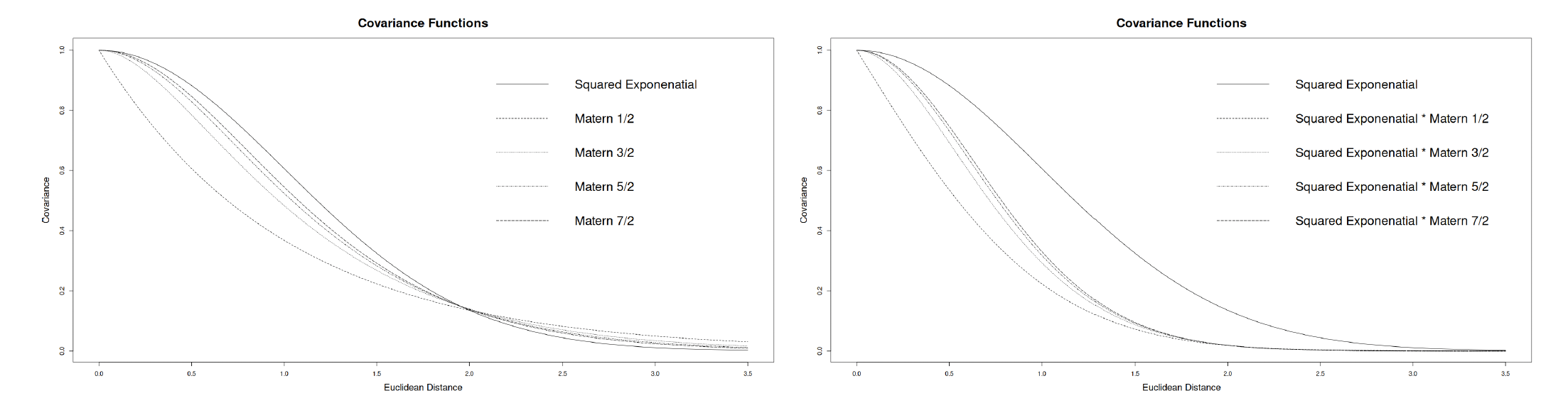
   Furthermore, by multiplying the formulas of different covariance functions, it is possible to combine them to obtain new and more expressive kernel functions. Multiplying kernels together is the standard way to combine two kernels, especially if they are defined on different sets of inputs. Figure 1 shows how the covariance decreases as the distance increases according to the different function presented and their combinations.

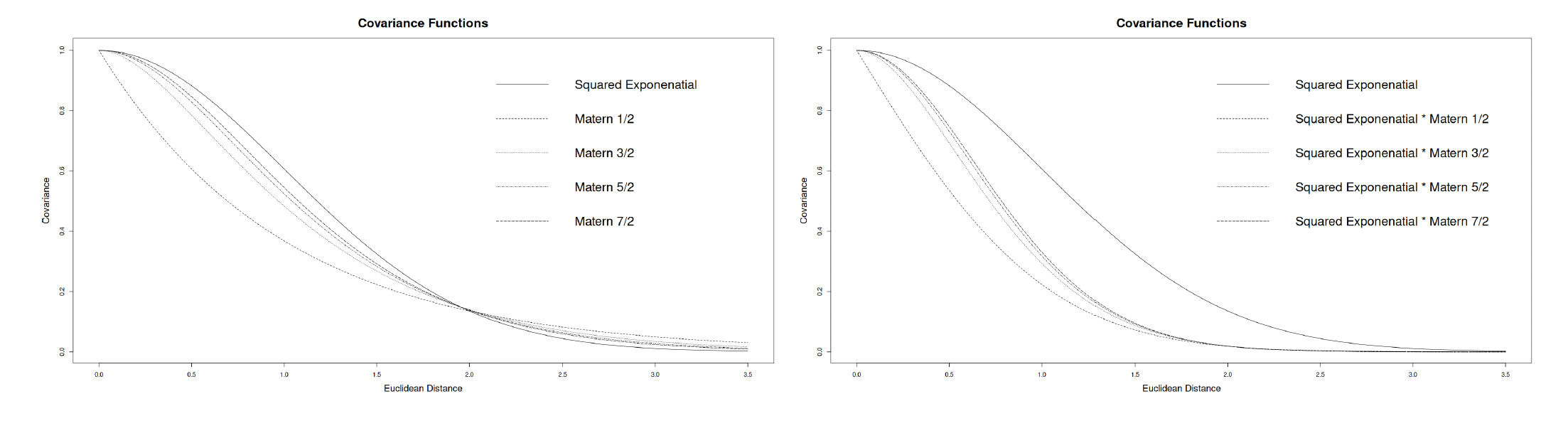
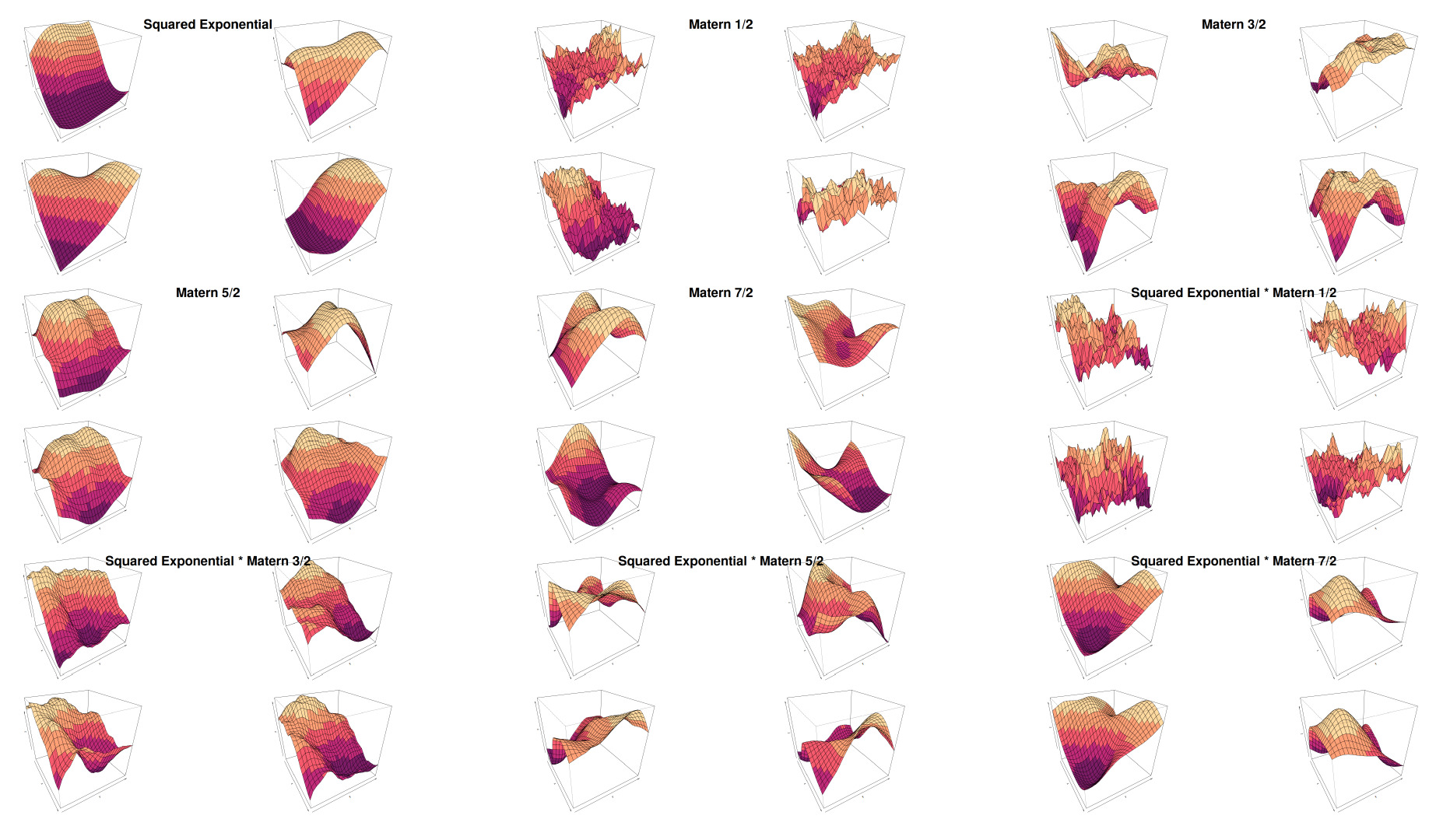
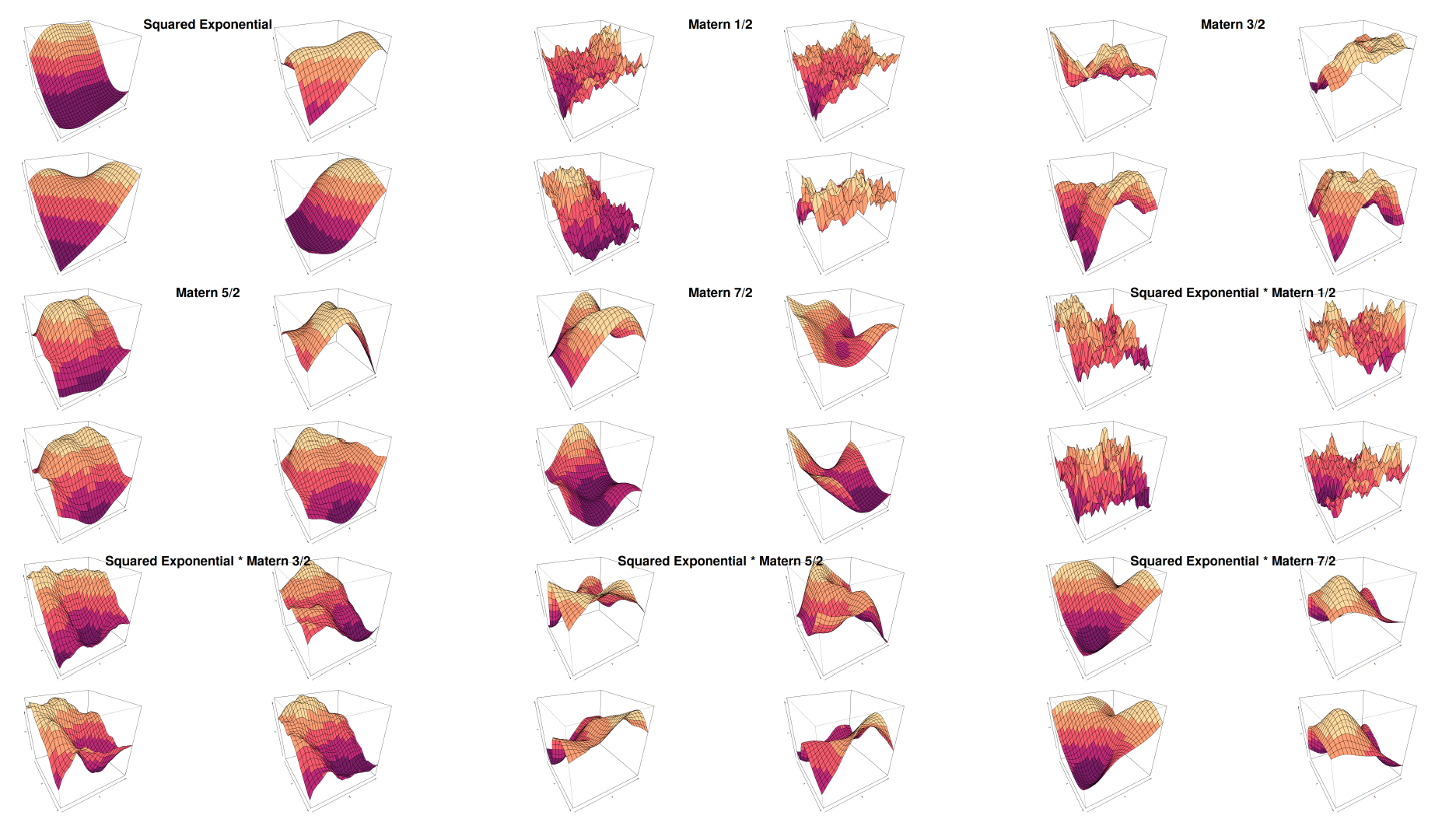
We can see that in Figure 2 the choice of the covariance kernel controls the smoothness and the structure of the sampled surface:

• Squared exponential: A smooth kernel.

• Matérn kernels (1/2, 3/2, 5/2, 7/2): These kernels introduce varying levels of smoothness—as the order increases, the surface appears less jagged. This is expected as the squared exponential kernel is defined as $\lim_{\rho \to \infty} \text{Matérn}(\rho) = \text{squared exponential}$.

• Combination kernels: These kernels represent composite kernels that combine features of two underlying covariance structures.

This grid of surfaces demonstrates the flexibility of GPR under different covariance kernels and their combinations. In the inverse Wishart regression context, the covariance structure would itself be random, meaning these surfaces could reflect different realizations of the posterior Gaussian process, accounting for uncertainty in the kernel parameters. This flexibility allows Gaussian processes to adapt both the functional form and covariance to better fit the data.

4.4. Gaussian process with inverse Wishart–distributed covariance function

We recap here how the aforementioned items are combined to define a Gaussian process:

$$f(X) \sim GP\big(0 , S \big),$$

where

$$S \sim IW_{p} \big(n\ ,V \big).$$

Thus, $S$ is inverse Wishart distributed, with $n$ degrees of freedom and a scale parameter $V$ that corresponds to a $p*p$ matrix equal to one of the kernels mentioned above (where $p$ equals the number of observations and $n \geq p$).

4.5. Gaussian processes as regression tools

Expanding on the theoretical foundations previously explained, we can frame Gaussian processes in the context of regression. As mentioned, GPR is a Bayesian technique, meaning that the learning phase is performed through an informative update of prior beliefs. In Bayesian statistics, in fact, the model elicits its knowledge about a phenomenon and then blends that initial information with the data observed, thus updating its assumptions in light of new evidence.

In our GPR formulation, prior knowledge is related to the form that the target function can assume, and thus, it can be expressed in terms of the kernel. Sampling from a multivariate normal distribution, with a selected kernel, valued with a realization of the inverse Wishart, we have a prior realization of our process—in other words, a possible functional form of the target variable according to our prior knowledge.

Following a Bayesian framework, the inference process is then performed in the following way:

1. Select the most appropriate kernel and the prior distributions for the kernel parameters. This represents the probabilistic model that describes the initial assumptions (priors) regarding how the data and parameters are generated.

2. Perform inference over the parameters by sampling through the observed data. By feeding a properly stated model into an inference engine, it is possible to sample realizations of the posterior distribution of parameters.

3. With the posterior distribution in hand, it is possible to sample from the full predictive distribution realizations of the target variable for new and unseen inputs.

Operationally, let $X$ be an $n * 1$ matrix, i.e., a column vector, in which every row is an input point $x_i, i = 1...n$ of the function. We first compute the variance-covariance matrix by applying the kernel function to each pair of data points:

$$\small{ K(X,X') = \begin{bmatrix} K({x_{1},x_{1}'}) & K({x_{1},x_{2}'}) & ... & K({x_{1},x_{n}'}) \\ K({x_{2},x_{1}'}) & K({x_{2},x_{2}'}) & ... & K({x_{2},x_{n}'}) \\ \vdots & \vdots & \ddots & \vdots \\ K({x_{n},x_{1}'}) & K({x_{n},x_{2}'}) & ... &K({x_{n},x_{n}'}) \\ \end{bmatrix}, }$$

where $K$ represents our kernel of choice. At this point, upon defining the degrees of freedom of the inverse Wishart $n$, we can sample a covariance matrix from such a distribution. To keep things simple, we set this parameter to the total number of input values plus 2. This is done because of statistical reasons to guarantee the existence of the expected value of the inverse Wishart distribution (Eaton 2007). After this, we set the mean function $m(x)$ equal to zero and use the sampled covariance matrix to generate realizations of prior functions for Gaussian processes with an inverse Wishart covariance function, $N(0, IW_{p}(n,K(x,x')))$.

However, understanding the behavior of the prior functions under different kernel choices is only part of the work. After collecting evidence, i.e., having some data points, the learning task consists of calculating the Gaussian prior conditioned on the observations.

Here we want to focus only on the practical aspect of the method, so we can lay the intuition. We defer to Rasmussen and Williams (2005) for a proper theoretical explanation. Intuitively, conditioning on a set of values does not alter the Gaussian nature of the process that is generating the functions. Hence, the posterior distribution corresponds to a Gaussian process conditioned on the observations.

More formally, we can prove that the conjugate^[5] nature of the Gaussian process prior and the Gaussian likelihood allows us to calculate a closed form for the posterior distribution from which we can sample. Even more intuitively, the probability distribution of the target functions is assumed to be Gaussian and likewise the prior. By applying the Bayes theorem, the posterior distribution of the functions is still Gaussian but embeds the knowledge gained from collecting more observations. Furthermore, the final expression will correspond exactly to the prior Gaussian process conditioned on the observations.

It is exactly the statistical properties of the conditioned normal distribution that allow GPR to be employed in a Bayesian regression context.

4.6. Gaussian process regression example

In this section let’s look at a brief example of how a GPR exercise works. For the sake of simplicity, we will consider a 1-D regression problem, where for each input $x$ there is an output $y$ through an unknown function $f(x)$. Let’s assume that we have the input data points $(x_1,\dots,x_n)$ and we want to find the regression function $\hat{f}(x)$ that estimates the real but unknown data-generating function $f(x)$.

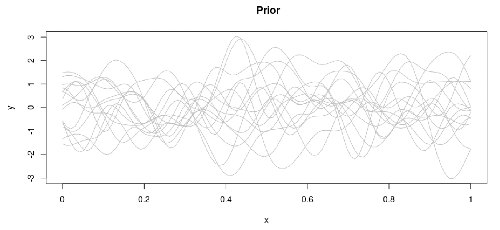
Let’s further assume that these points follow a multivariate normal distribution. We start by randomly drawing from the prior distribution over functions (Figure 3) specified by a particular Gaussian process^[6] with inverse Wishart–distributed covariance.

This constitutes our prior distribution, and it represents our beliefs on the form of the target function before actually having seen any data points.

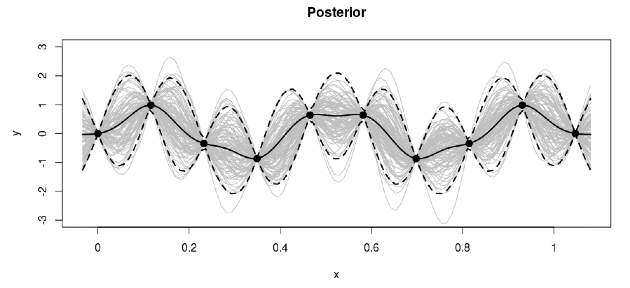
As is normal in a Bayesian context, we then focus our attention on the actual data points (Figure 4). This allows us to retain only the functions that actually pass through the data $\{(x_1, y_1),\dots,(x_n,y_n)\}$.

The combination of the prior and the data leads to the posterior distribution over functions.

This simple example constitutes a very high-level view on how the inference process works in the context of regression. It is, in fact, possible to generalize the process to specify different prior distributions and even extend the process in more than one dimension, as we will see in the next sections.

5. Claim liabilities estimation

One of the main areas of study in actuarial science is claim liabilities estimation. In this regard, we can identify two macro areas of modeling approaches adopted: deterministic and stochastic. Over the past few years, stochastic approaches have grown in importance, especially in connection with other areas of risk management. Nowadays, not being able to give a range around best estimates may lead not only to a downgrade from insurance credit agencies but also to regulatory scrutiny (Brehm et al. 2007). One of the most popular stochastic reserving methodologies is based on regression approaches through parametric linear models, whereas research on nonparametric models, although increasing, is still not as extensive. As previously mentioned, our research falls under the category of nonparametric approaches. We develop a technique based on GPR in order to produce a stochastic estimation of claim liabilities. Furthermore, we show how to review the findings in light of the development factors so as to provide a bridge to more traditional actuarial methodologies.

5.1. Restating the claims reserving problem

The objective of the study is to estimate the ultimate claim liabilities, given the data, organized in a long-format table with origin and development periods presented as columns—thus fitting claims figures in terms of accident years (AYs) and development periods (DPs) in a typical machine learning fashion. Such a structure could be built based on cumulative or incremental data. We will call cumulative data $C_{w,d}$ and incremental data $q_{w,d}$, where w indicates the origin period and d the development period.

Alongside claim amounts, we also focus our attention on the amount of earned premium for each origin period $P_w$. This will help us define the LR as losses (cumulative or incremental) divided by premium amounts.

As every practitioner knows, the traditional analysis is carried out via the so-called run-off triangle, a matrix representation (or, equivalently, a wide-format table) where origin periods are reported on the rows and development periods on the column. We understand that not looking at claims data in that way may be confusing at first, but due to the nature of the method employed, and to avoid confusion at later stages, we will abandon the traditional run-off triangle view in favor of a long table view. Moreover, data in a long format offer additional flexibility: in principle, further covariates—i.e., further columns—could be added to the data, allowing us to capture dynamics that more traditional models will miss—e.g., the calendar year or to model inflation assumptions or features that reflect particular business details. For additional details, we recommend Parodi (2013).

That being said, the data used for our analysis will have the following shape:

The target of the analysis, then, is to predict future observations, i.e., observations for which $w + d > n$, given observed claims, i.e., $w + d \leq n$. Therefore, we want to estimate a function such that $f(w,d) = q_{w,d}$, where $f(w,d)$ is a GPR.

As opposed to previous research on the subject (Lally and Hartman 2018) and following the framework of Renshaw and Verrall (1994), we focus our attention on estimating incremental payments (or incremental LRs) instead of cumulative. This is to avoid correlation issues during the modeling phase: it is assumed, in fact, that incremental amounts are independent, whereas cumulative ones are not. Each cumulative amount depends on the payments made at the previous development periods.

5.2. Graphical representation of claims data

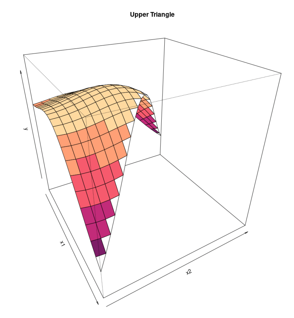
Before starting our analysis, we present an alternative 3-D graphical representation of claims data. The origin period will be on the x-axis, the development period on the y-axis, and the actual incremental claim payments (or LRs) on the z-axis.

We do this to clarify, one more time, the framework of the analysis: we have a surface, and we want to find a function that best approximates the observed data. More specifically, said function is a nonparametric GPR.

In Figure 5 and Figure 6, we show what a dataset of claims data looks like.

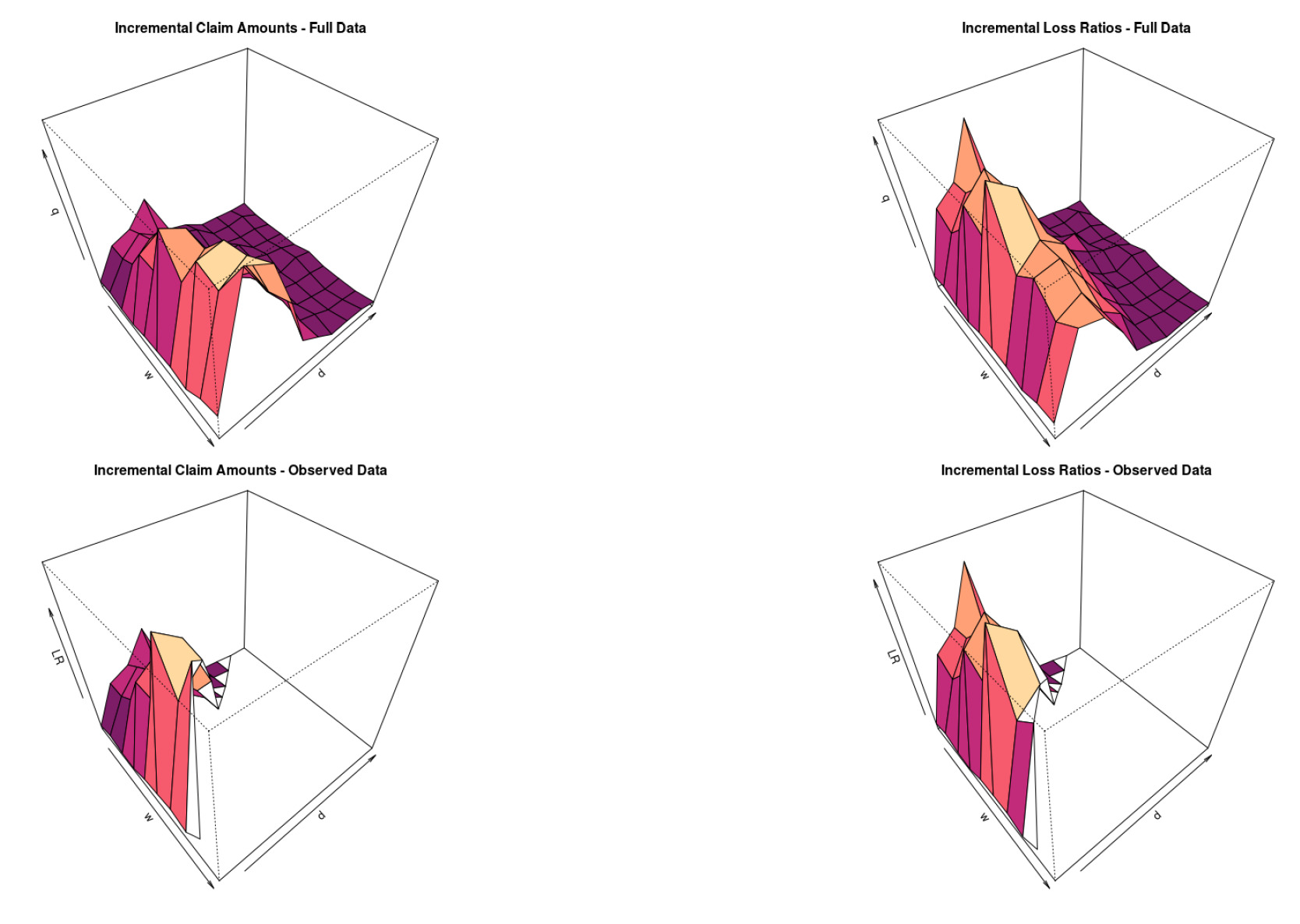
The first row shows the full dataset, whereas the second row shows the data we have in order to fit the GPR.

6. Fitting GPRs on reserving data

In this section, we present the framework followed for the general case, highlighting the most relevant results, and in the next section we show a specific and reproducible full-worked example. We fit the presented models on both incremental claim amounts and incremental LRs on a dataset composed of 24 publicly available triangles from the National Association of Insurance Commissioners (NAIC) Schedule P (Meyers and Shi 2011) and analyze the results.

The data contain fully developed triangles of the major personal and commercial line^[7] portfolios of U.S. property and casualty insurers. The claims data come from Schedule P—Analysis of Losses and Loss Expenses in the NAIC database.

Before actually fitting the models, we performed several data quality, data cleaning, and preprocessing steps to ensure that the data were actually suitable for our purposes. As a result, we filtered out many triangles that we deemed unsuitable.^[8] This was necessary because we have a fairly sophisticated model with many parameters, and therefore it is important to have data that are capable of supporting the training process.

We present in Table 2 an example of data used in the analysis. As previously mentioned, the data supplied to the model are not in wide form (or triangular form) but in long form.^[9]

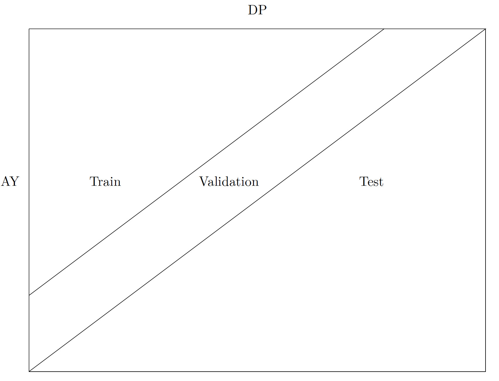
Consistent with the long format, we follow the traditional machine learning work flow for fitting a GPR. For each triangle in the dataset, we filter out the data of the lower triangle, i.e., the test set; this represents data that would not be available in a true business setting. The remaining data points, i.e., the upper triangle, are then split into a training set and a validation set. The validation set corresponds to the last two diagonals, and the training set is instead composed of all the remaining data (a smaller upper triangle without the two most recent diagonals) (see Figure 7).

Then, for every triangle, we perform a grid search looking for the best prior distributions and parameters. We fit every combination on the training set and we validate them on the validation set. The validation is carried out according to two criteria, quality of point estimates and quality of the resulting stochastic distribution, in a similar fashion as the evaluation methodology proposed by Meyers (2015). To evaluate the quality of the point estimates we look at the root-mean-square error (RMSE). The quality of the stochastic properties is analyzed by calculating the observed reserve percentile on the estimated distribution and then tested with the Kolmogorov–Smirnov (K-S) test for the uniform distribution.

6.1. Model specifications and parameters

This section is dedicated to the specifics of the model and all the details surrounding the fitting process adopted for every triangle.

As outlined in Section 5, we assume that the standardized incremental paid claims, $q'(w,d)$, are the output of an unknown process that we want to estimate with the implementation of a GPR. More specifically, we assume that $$q'(w,d) \sim GP\big(0, IW(n+2,K(w,d) \big).$$ The standardized incremental paid claims can therefore be modeled via a Gaussian process with a mean of zero and where the covariance function is assumed to have an inverse Wishart distribution centered on a kernel of choice.^[10] As outlined, the mean of the process is assumed to be equal to zero. Therefore, the behavior of the process is entirely specified by the covariance function $K(w,d)$.

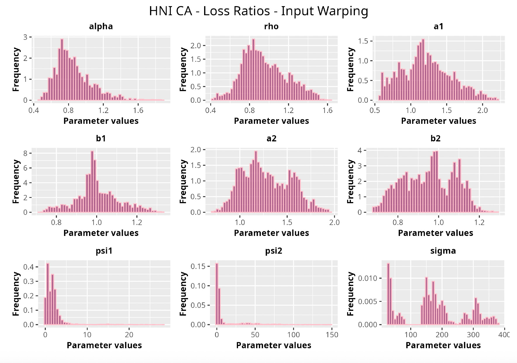
6.2. Inputs

First, we discuss the inputs of our model, i.e., the origin period, $w$, and the development period, $d$. These are the only two inputs of the model that determine the value of the claims $q(w,d)$ or, in the graphical representation, the value of the elevation of the surface of the multivariate Gaussian distribution at $w$ and $d$.

These two values may have very different scales—e.g., in Table 2 we have $w$ $\in [1988, 1997]$ and $d$ $\in [1, 10]$. It is necessary to implement a standardization algorithm to ensure they both are on the same range and are comparable.

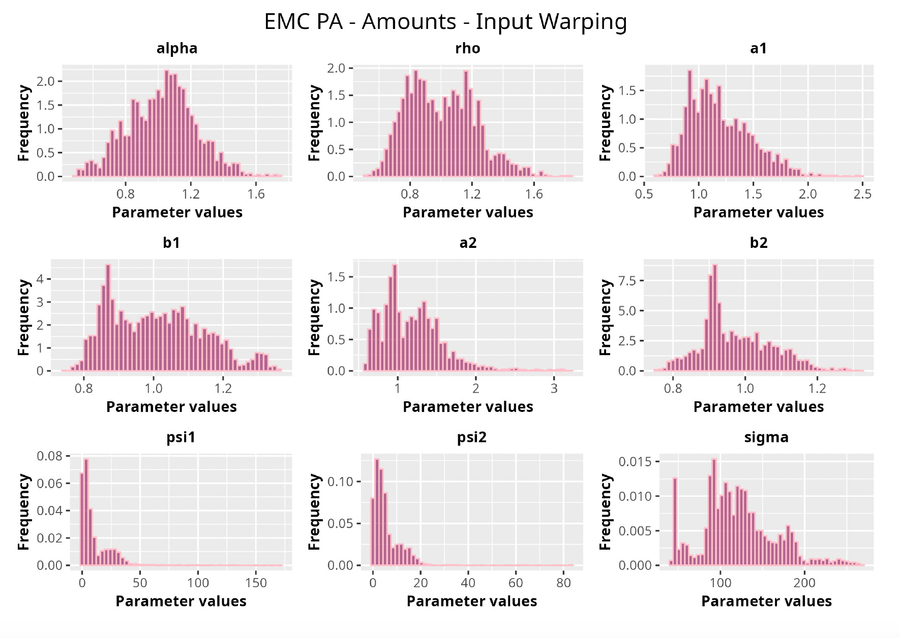
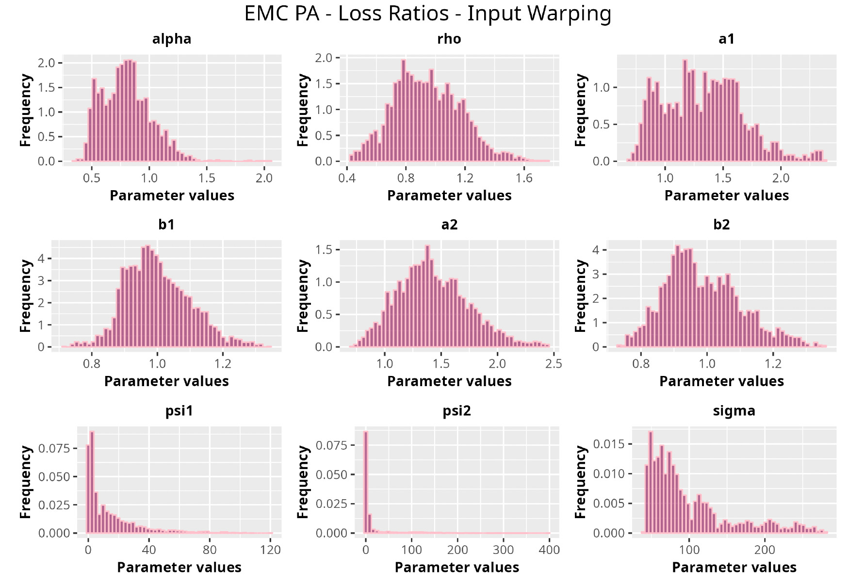
Following the suggestion of Snoek et al. (2014), we accomplish this by performing an operation called input warping. In a nutshell, input warping is a sophisticated two-step standardization technique that helps produce more stable and reliable results when adopting machine learning techniques. We measure its impact by running the same procedure twice—first employing the input warping transformation and then without this extra data preparation step.

Input warping works by employing the beta cumulative distribution function (CDF), which takes as input a value between zero and 1 and returns again, as output, a value between zero and 1. After operating an initial min-max normalization, we can feed the values into the selected beta CDF to ensure consistency between the two scales. Here we describe the procedure in greater detail:

$$\begin{aligned} & w' = \frac{w-w_{min}}{w_{max} - w_{min}}, \\ & w'' = I_{w'}(a_w, b_w), \\ & d' = \frac{d-d_{min}}{d_{max} - d_{min}}, \\ & d'' = I_{d'}(a_d, b_d), \end{aligned}$$

where $w$ and $d$ are the actual origin period, and the development period inputs $I_{x}(a, b)$ is the CDF of the beta distribution and $a_w, b_w, a_d, b_d$ are real parameters.

We can think of this process as a sophisticated normalization technique controlled by the parameters $a_w, b_w, a_d, b_d$. Finally, $w''$ and $d''$ are the values imputed to calculate the covariance function. As mentioned, we will provide results of the analysis using $(w', d')$ and $(w'', d'')$ to quantify how this step contributes to the final results.

6.3. Covariance functions

Having established the final transformation for the inputs, we can turn our attention to the covariance functions used in the model. We implement the covariance functions outlined in Section 4.2 with some minor modifications. They all depend on the same set of parameters; however, there will be some differences in how the actual calculations are carried out.

The distance $d$ between $w''$ and $d''$ (or between $w'$ and $d'$) will be calculated as

$$\begin{aligned} dist = \sqrt{\psi_w|w''|^2 + \psi_d |d''|^2}, \end{aligned}$$

for which $\psi_w$ and $\psi_d$ are real parameters and the operator $|\cdot|$ is the norm of a vector. In addition, we also introduce a real parameter, $\sigma$, to be added to the diagonal of the covariance matrix, so as to incorporate a supplementary source of noise.

In the worked examples presented next, we tested different covariance functions and several combinations of them, effectively treating the specification of this function as a hyperparameter of the model.

6.4. Outputs

The target variables of the two modeling exercises are the standardized future paid incremental claim amounts, $q'(w,d)$, and the standardized future incremental LRs, $\frac{q'(w,d)}{P_w}$.

We can then establish the following relations:

$$\begin{aligned} q'(w,d) = GP\big(0, IW(n+2,K(w,d) \big), \\ \frac{q'(w,d)}{P_w} = GP\big(0, IW(n+2,K(w,d) \big). \\ \end{aligned}$$

It is noteworthy to observe that the mean of the Gaussian process is actually set equal to zero, a choice that will greatly simplify the calculations without having any impact on the actual estimates. First, we need to standardize the claim values before the fitting process. This is easily done by subtracting the mean and dividing by the standard deviation.

All the incremental values in the same triangle will be subject to the same standardization process—i.e., we select one mean value and one standard deviation value for each triangle.

We do not need to worry about estimating the mean of the process, as we are dealing with a multivariate Gaussian distribution that is entirely determined by the chosen covariance function. This means that the output of the model depends entirely on the set of parameters $a_w, b_w, a_d,$ and $b_d$, which control the input warping; the set $\psi_w, \psi_d, \alpha$, $\rho$, and $\sigma$ instead determine the value of the covariance and also the kernel shape.

These parameters are exactly what we are after and what we want to estimate. To do so we use a hierarchical Bayesian model implemented through the Stan (Stan Development Team 2022) programming language accessed from R (R Core Team 2021). The last detail to highlight is the possible range of outputs; because the estimated amounts will be the output of a Gaussian distribution, they could fall anywhere in the range $(-\infty, +\infty)$, which encompasses negative values. We do not operate any transformations, e.g., log transformation, to constrain the output to be a positive number. The rationale behind this choice is twofold. First, we are modeling incremental and not cumulative values, and negative incremental values can still make sense—e.g., the insurer may receive recoverables from several sources such as reinsurance, salvage, or subrogation. Second, it is beneficial to study and model the probability associated with such recoverables.

6.5. Model fitting

As briefly introduced, we fit the model according to the traditional machine learning workflow; hence we split the data (the upper triangle—in a long format) into training and test sets. For each triangle, the training set is composed of all the data for which $w + d < 1997$, i.e., the upper triangle less the last two diagonals.

The validation set, instead, is composed of all the data for which $w + d \in [1997,1998]$, i.e., the two most recent diagonals.^[11] Finally, actual performance will be computed on the lower triangle, i.e., $w + d > 1998$.

With this in mind, for every triangle we performed a grid search procedure looking for the optimal combination of prior distributions and parameters. We tried nine different covariance functions and 28 different sets of parameters, for a total of 252 different combinations of kernels/hyperparameters.

For each triangle, every model was evaluated against the validation set. We then selected the best combination of priors and parameters based on the RMSE and K-S criteria, as previously explained.

With this procedure, we were able to select a model for every triangle and perform an estimation that implicitly takes into account the peculiarity of different lines of business and the history of possibly different underwriting and reserving policies.

6.6. Results

With all the fit models at hand, we ran the prediction procedure for every triangle. As would be the case in a real business setting, we used the upper triangle to predict the lower one. Also, having the actual observed lower triangle available, we were able to test the procedure versus the real observed values. In Table 3, we show the weighted average of the RMSEs and the K-S p-value resulting from the prediction on all of the triangles, as well as the average RMSE and the K-S p-value calculated on traditional actuarial methods.^[12] We would like to note that we repeated the calculations for a total of four times. First, the model was run once on the amounts and once on the LRs, and second, those calculations were repeated with and without the input warping technique on the data in order to capture its effect.

As can be seen in Table 3, GPRs outperform the traditional chain ladder/overdispersed Poisson (ODP) method on both the RMSE and K-S metrics. The best performer turns out to be the GPR trained on incremental LRs with input warping: the resulting average RMSE is almost 40% less than the RMSE of the traditional chain ladder. Also, from a stochastic perspective, the GPRs produce superior results; we see where the observed reserve fell in terms of the percentile of the estimated predictive probability distributions. The expectation was for the percentiles across the entire dataset to be uniformly distributed, implying an unbiased prediction of the method. The K-S confirms this hypothesis for all the GPRs and rejects it for the traditional methods. As for input warping, its impact can be immediately appreciated. Where input warping is adopted, it brings clear performance gains, thus confirming the importance of the standardization step, especially on incremental reserving data where the domains of the input factors can be very different.

7. Application

In this section we demonstrate the results of applying the GPR procedure to five different triangles from different companies and lines of business:

• EMC Insurance Companies private auto (EMC PA) policies from 1988 to 1997

• EMC Insurance Companies other liability (EMC OL) policies from 1988 to 1997

• California Casualty workers compensation (CC WC) policies from 1988 to 1997

• Physicians’ Reciprocal Insurers medical malpractice (PRI MM) policies from 1988 to 1997

• Harco National Insurance Company commercial auto (HNI CA) policies from 1988 to 1997

The rationale behind this selection is that it consists of a wide range of lines of business and also triangles in which traditional methodologies work really well and triangles in which traditional methodologies do not provide satisfactory results.

Triangles in which standard methodologies work well provide a true performance comparison term for the GPR. Moreover, the ones unsuitable for traditional methodologies could show the potential of the GPR procedure to provide a method that can achieve good results with little external intervention.

We select the best GPR based on a grid search encompassing both the covariance function and the set of prior distributions. The search is carried out in the manner described in the model fitting section; the best-performing covariance function, for this specific triangle, turns out to be the combination between the Matérn 5/2 and the squared exponential functions with the input warping procedure. Moreover, carrying out the analysis on the LRs rather than the actual claim amounts seems to produce better results.

We compare the results of the GPR procedure using the chain ladder/ODP method with a gamma process variance. This is one of the more well-known stochastic frequentist methods with which to sample a predictive distribution of unpaid claims liabilities. Furthermore, we provide the observed amounts, thus testing both methods against the actual observed development.

We compare the results in Table 4, along the lines of three main metrics:

• The predicted mean reserve, so as to have an absolute metric of the amounts produced by the model

• The RMSE, in order to appreciate the error of the estimates

• The observed percentile, a value that reports the percentile of the observed reserve on the distribution of the estimates

As one can appreciate from the figures in Table 4, the GPR methodology outperforms by having a lower RMSE than the more traditional ODP method in all the trials, except for one case. It is worth noticing, however, that even in this single instance the GPR absolute percentage error on the observed values is 2.3%, whereas the ODP’s is 1.9%. The two methodologies are not drastically different.

Focusing on the stochastic metric instead, one can observe, by looking at the values for the observed percentile, how the GPR procedure produces distributions almost exactly centered on the observed value, hence having results less susceptible to random variability and therefore more reliable.

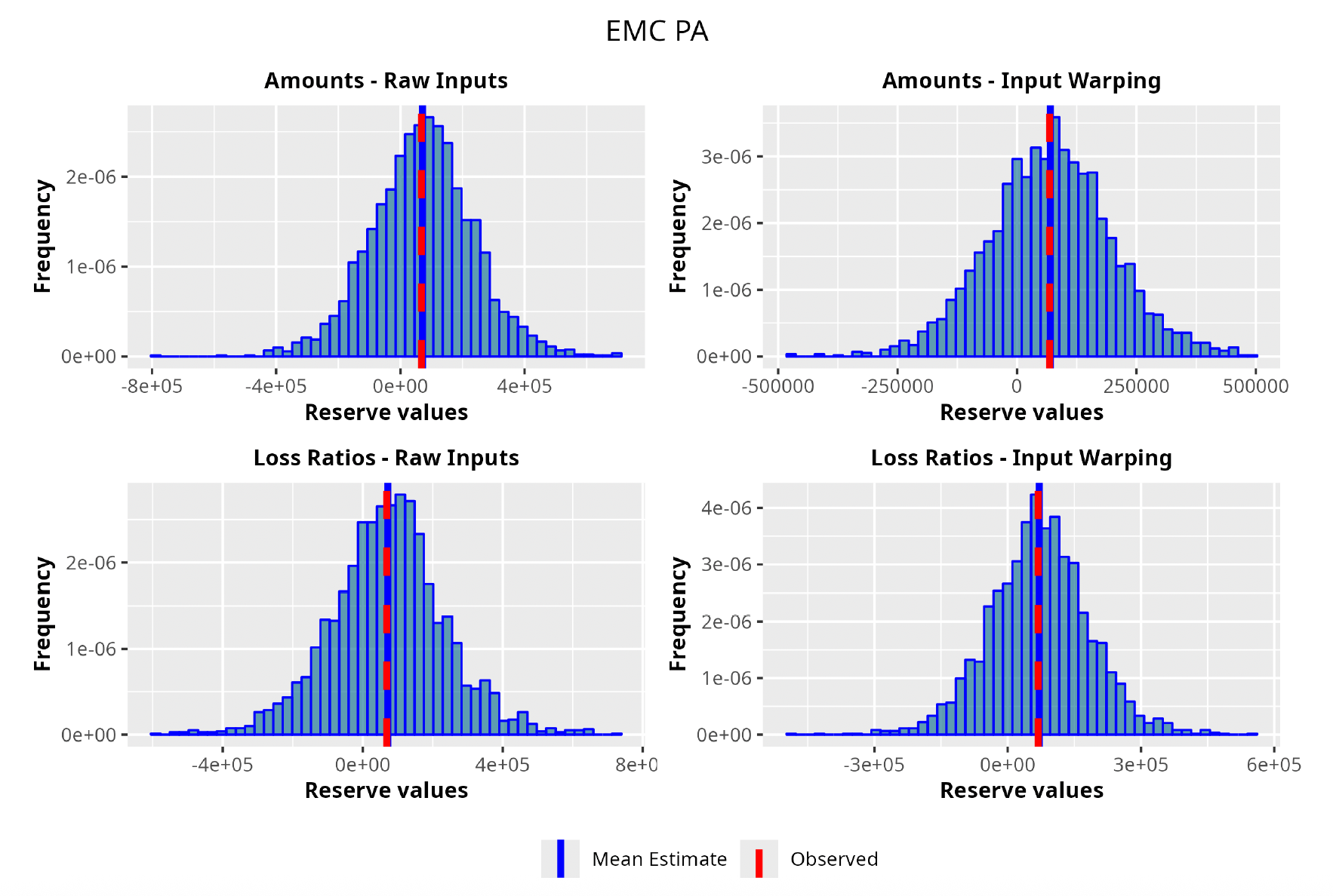
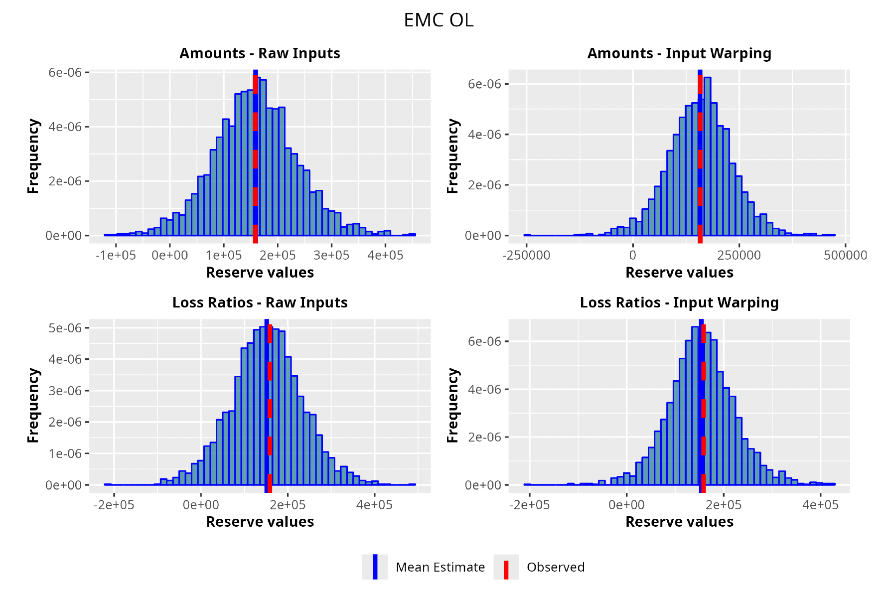
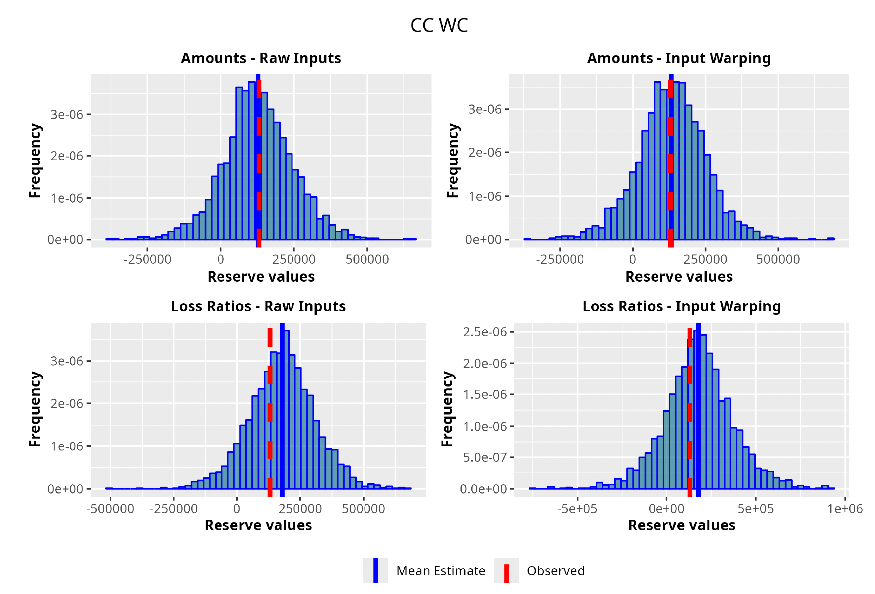
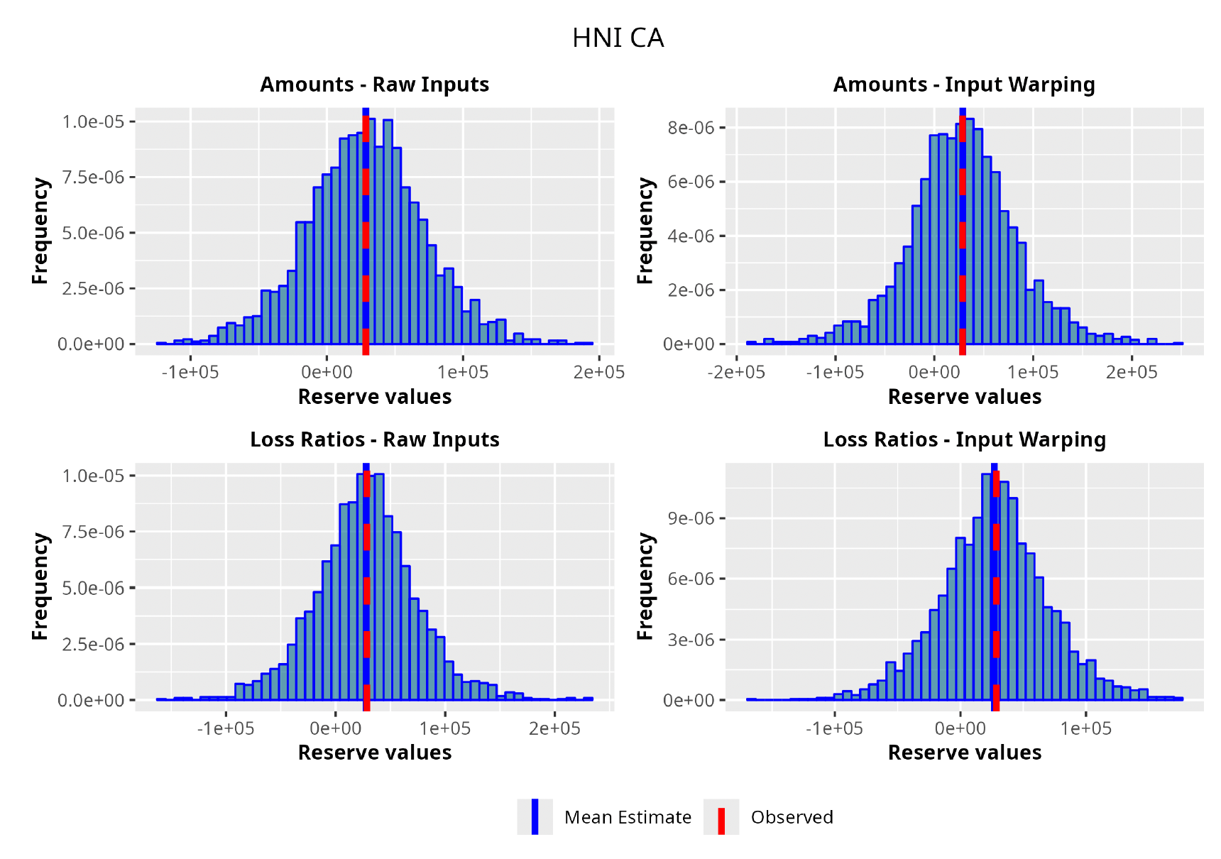
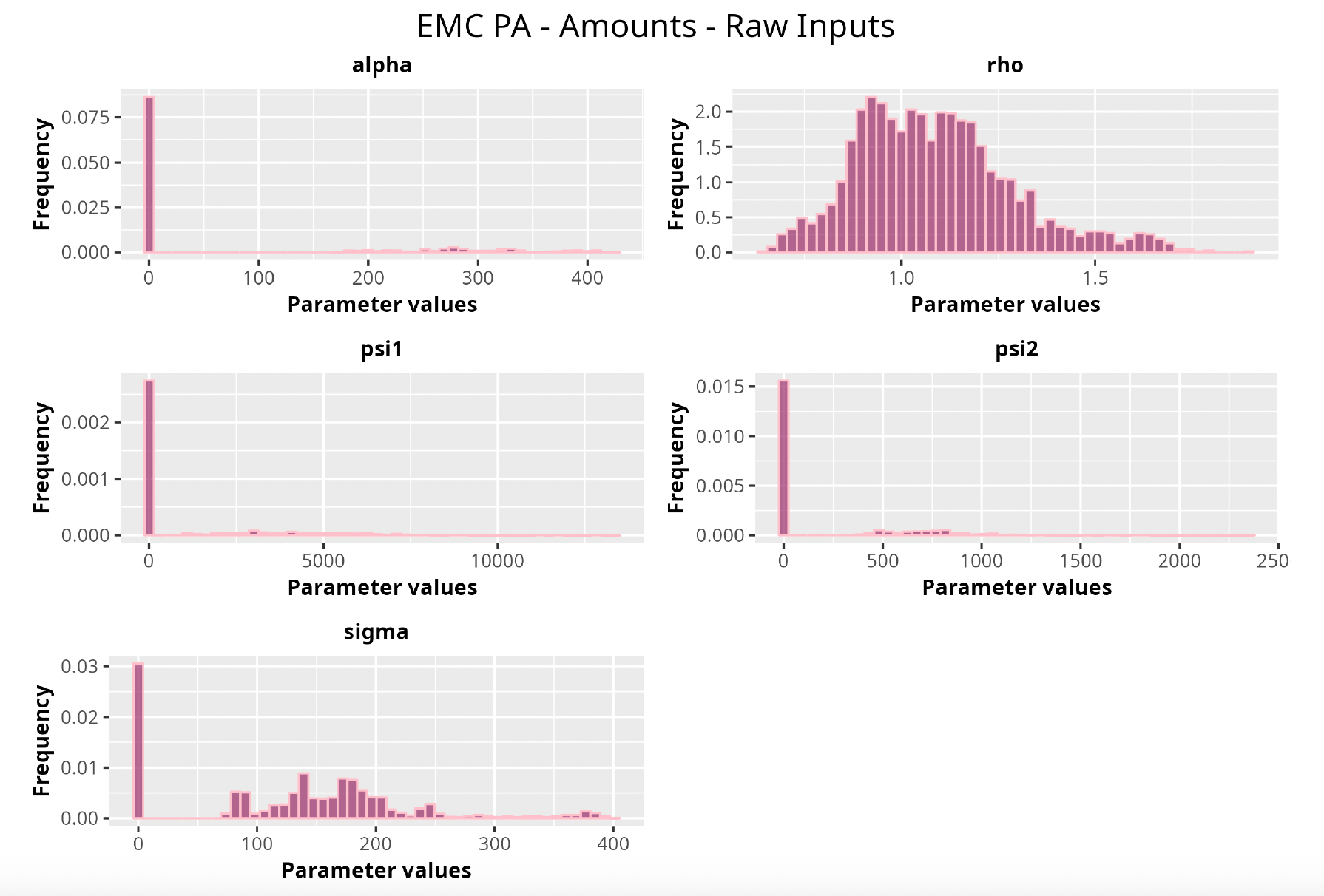
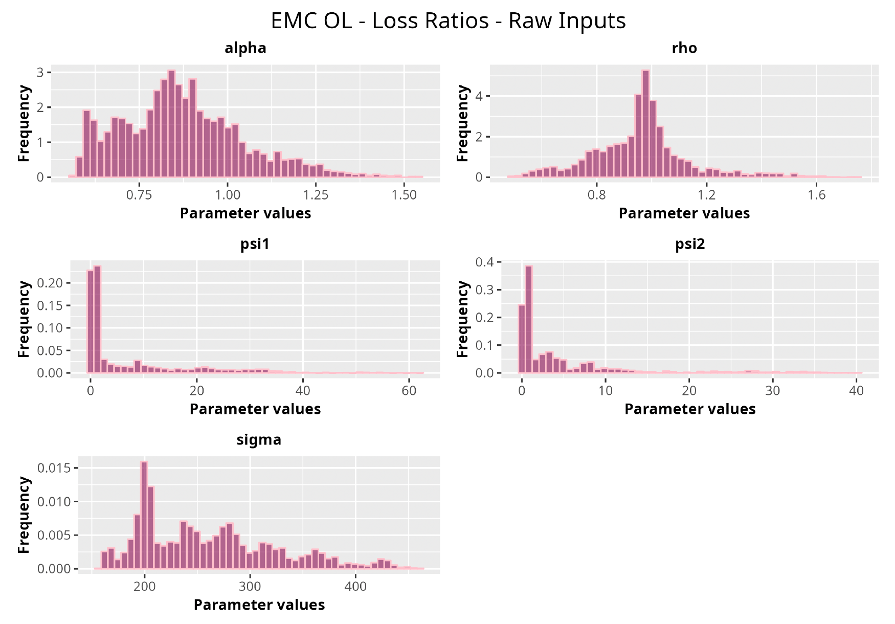
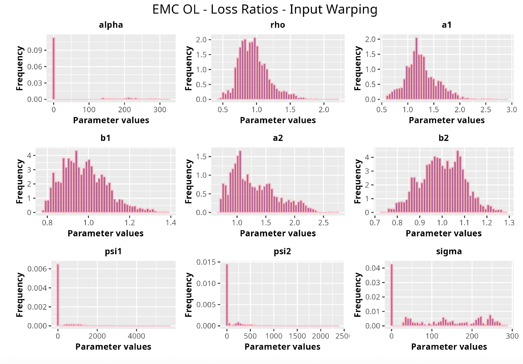
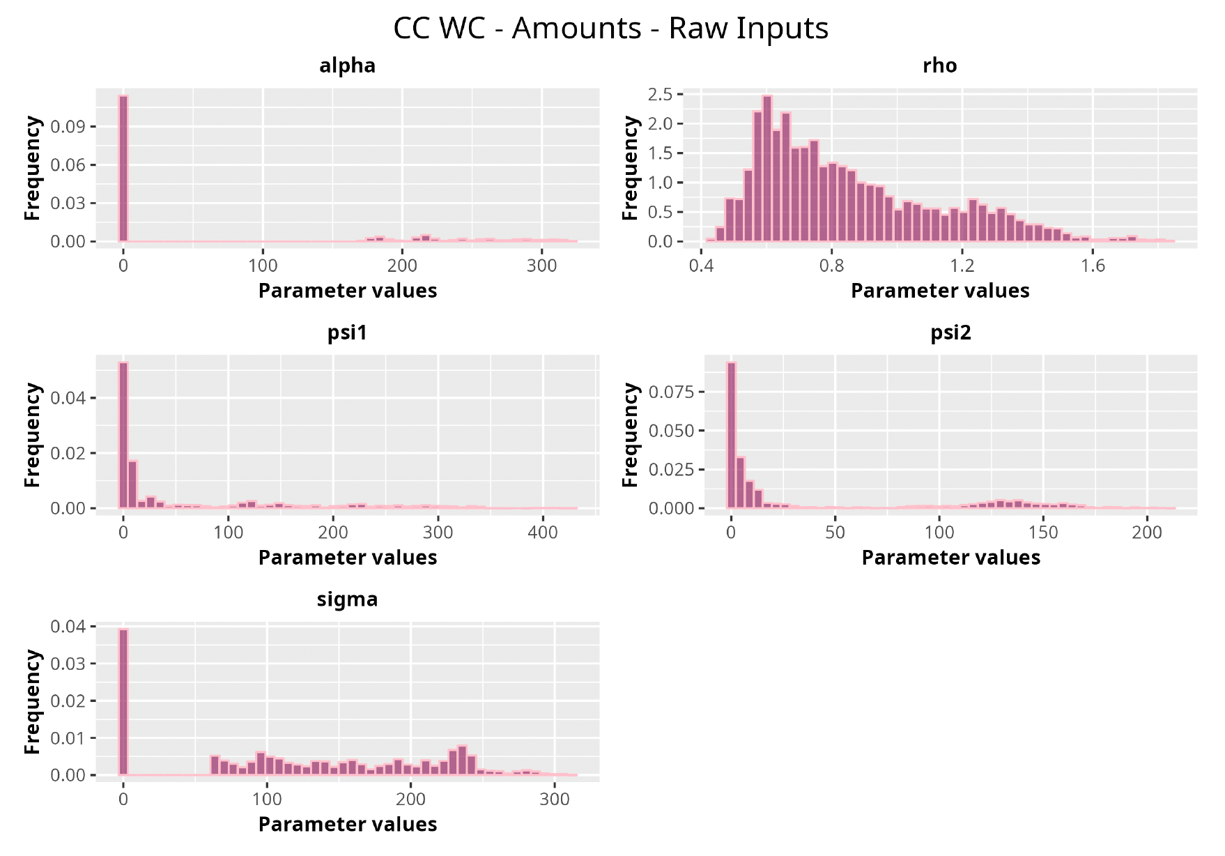
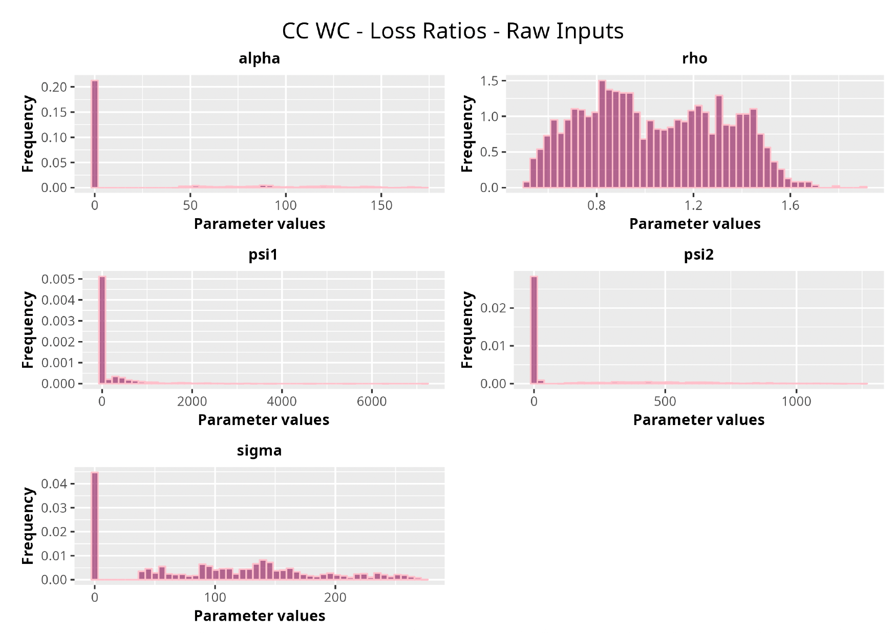
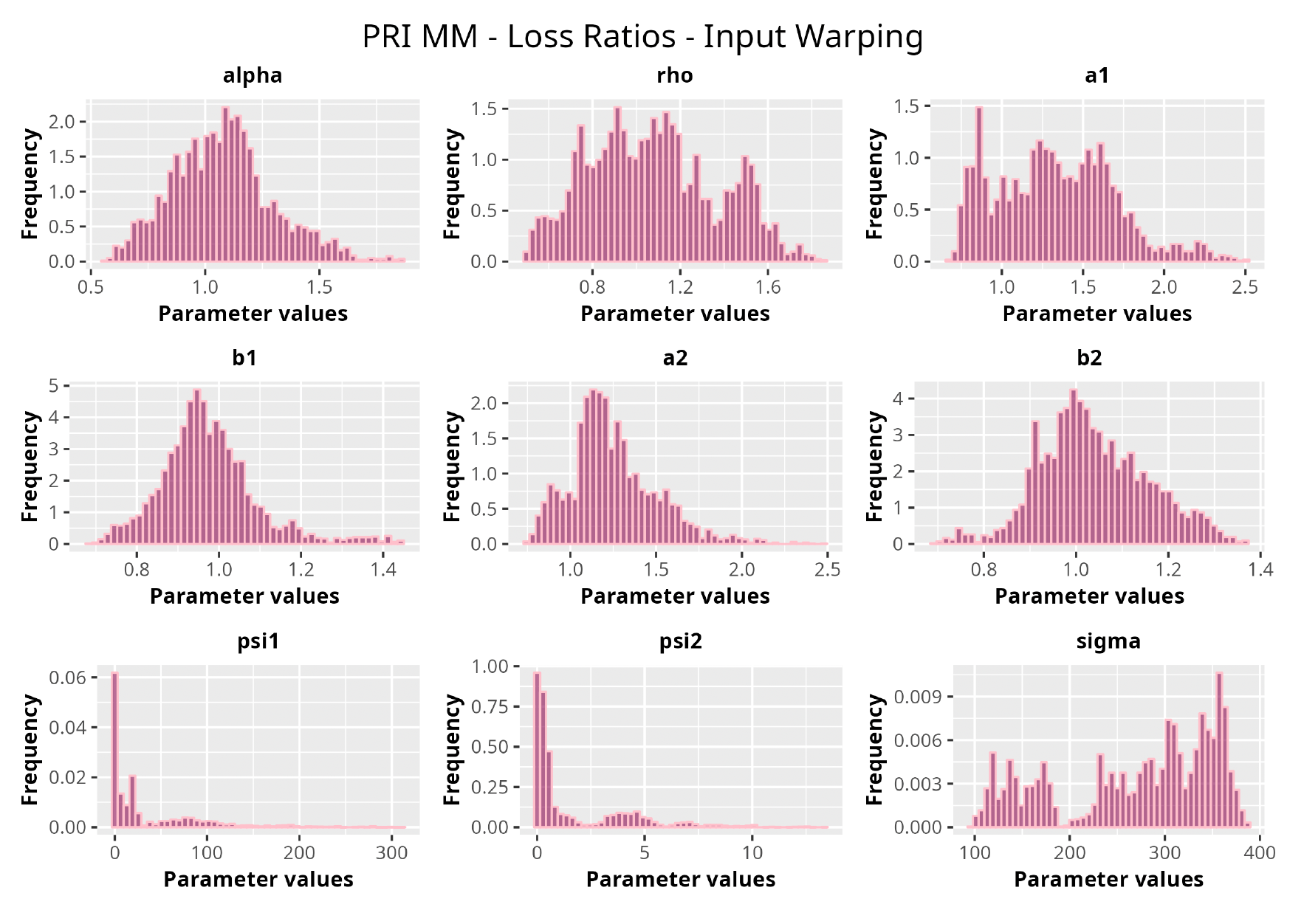
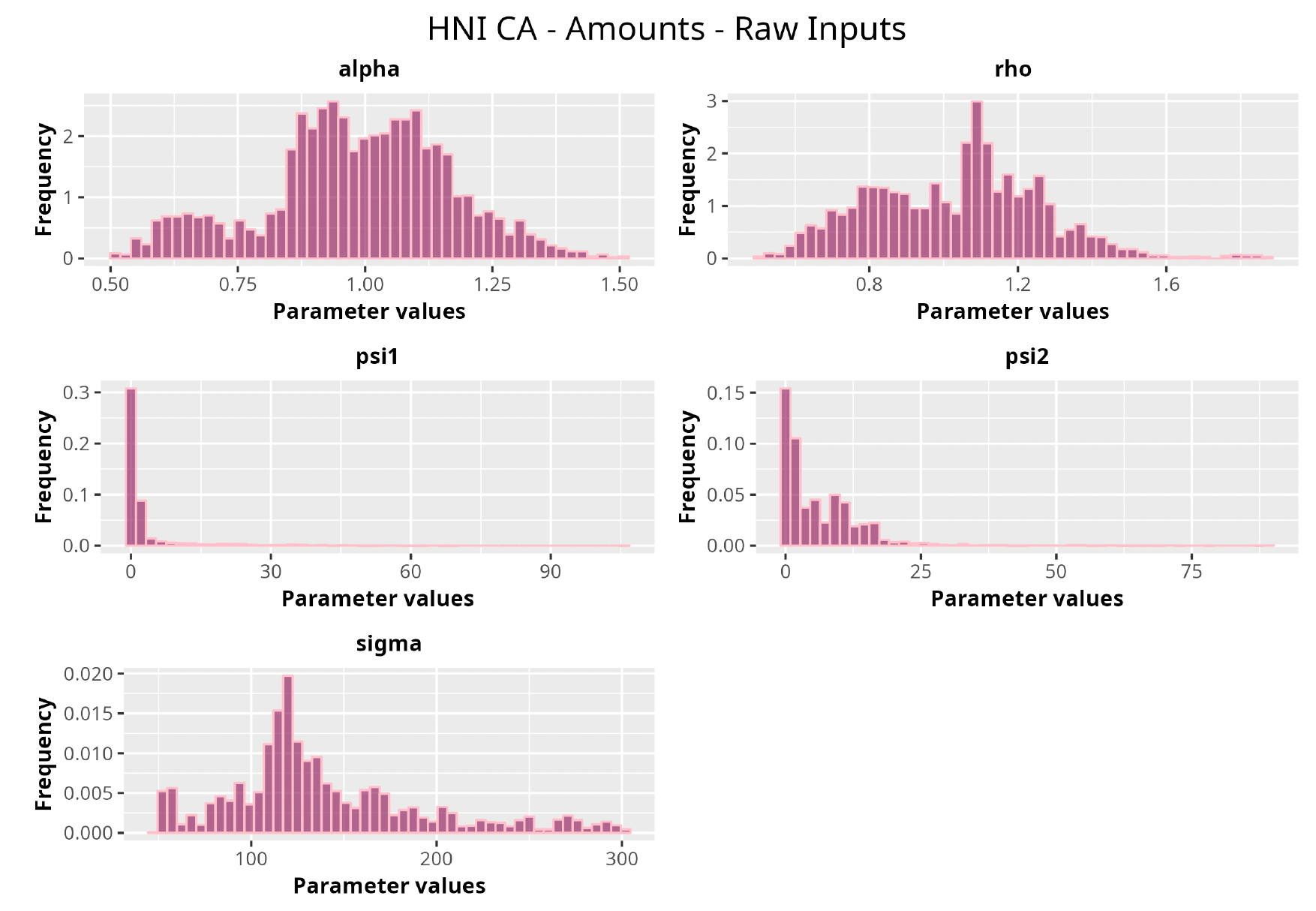
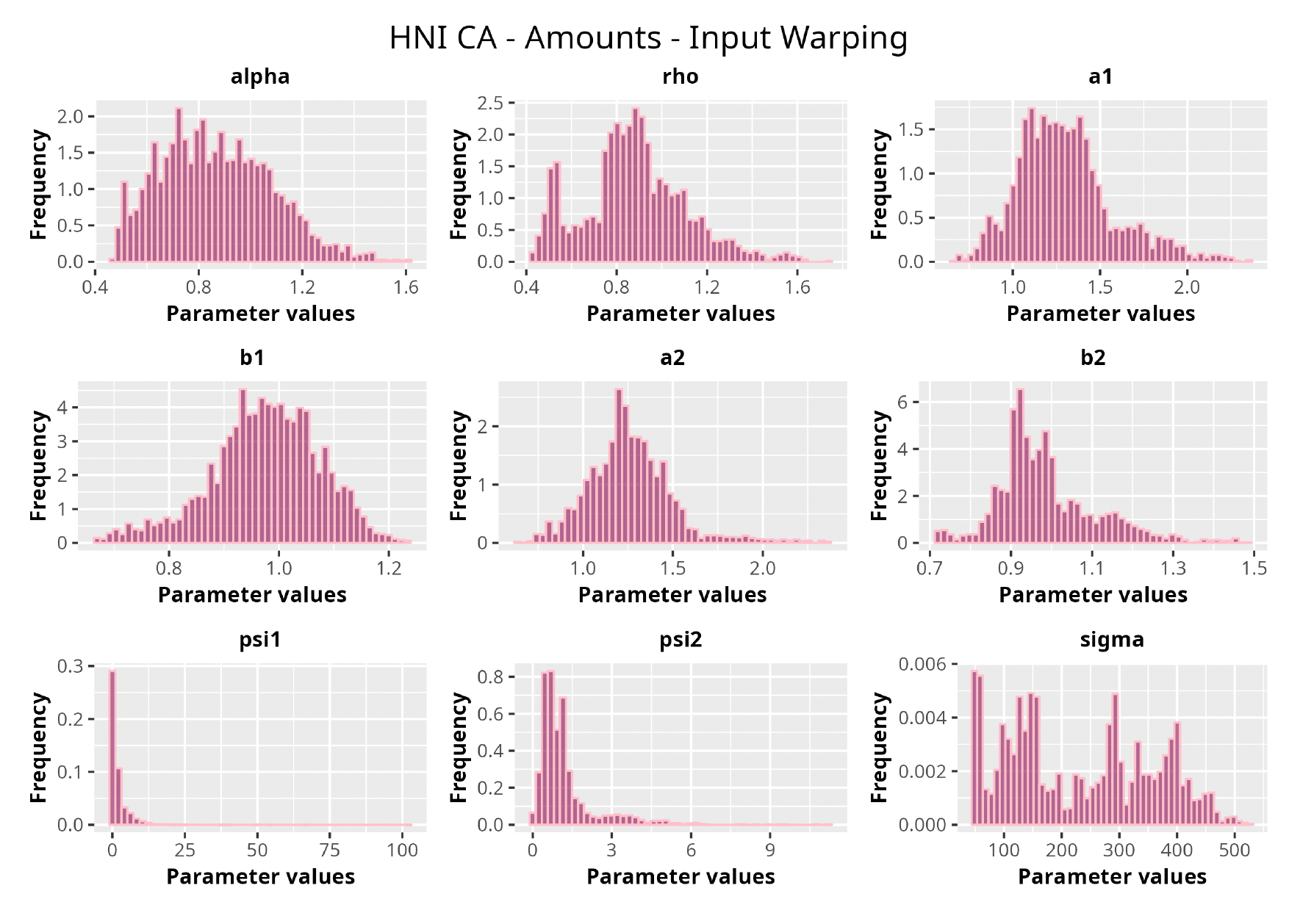
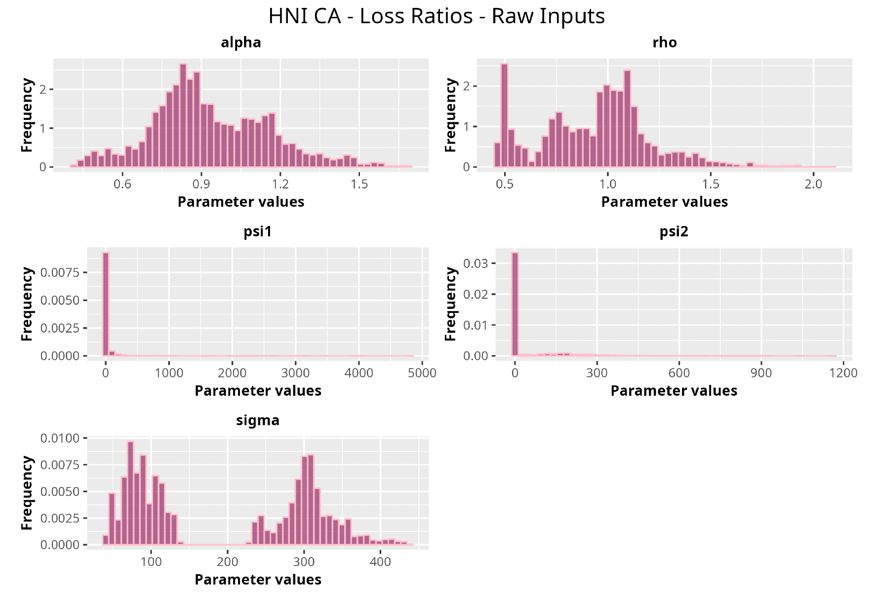
In the following plots (Figures 8 to 12), we show the predicted reserve distributions for each triangle and for each GPR procedure, i.e., LRs versus amounts and input warping versus raw inputs.

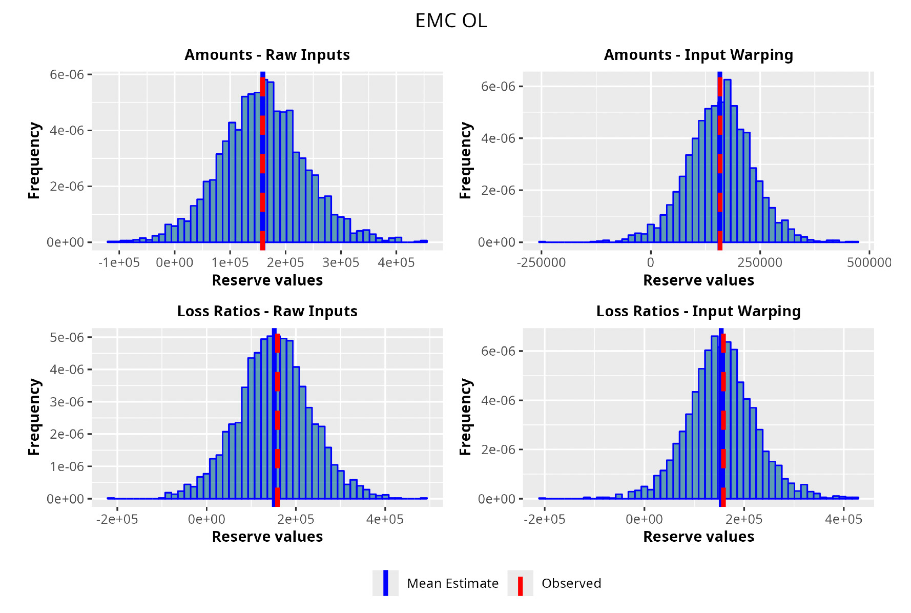
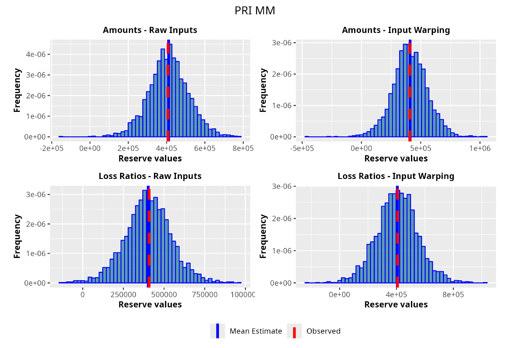
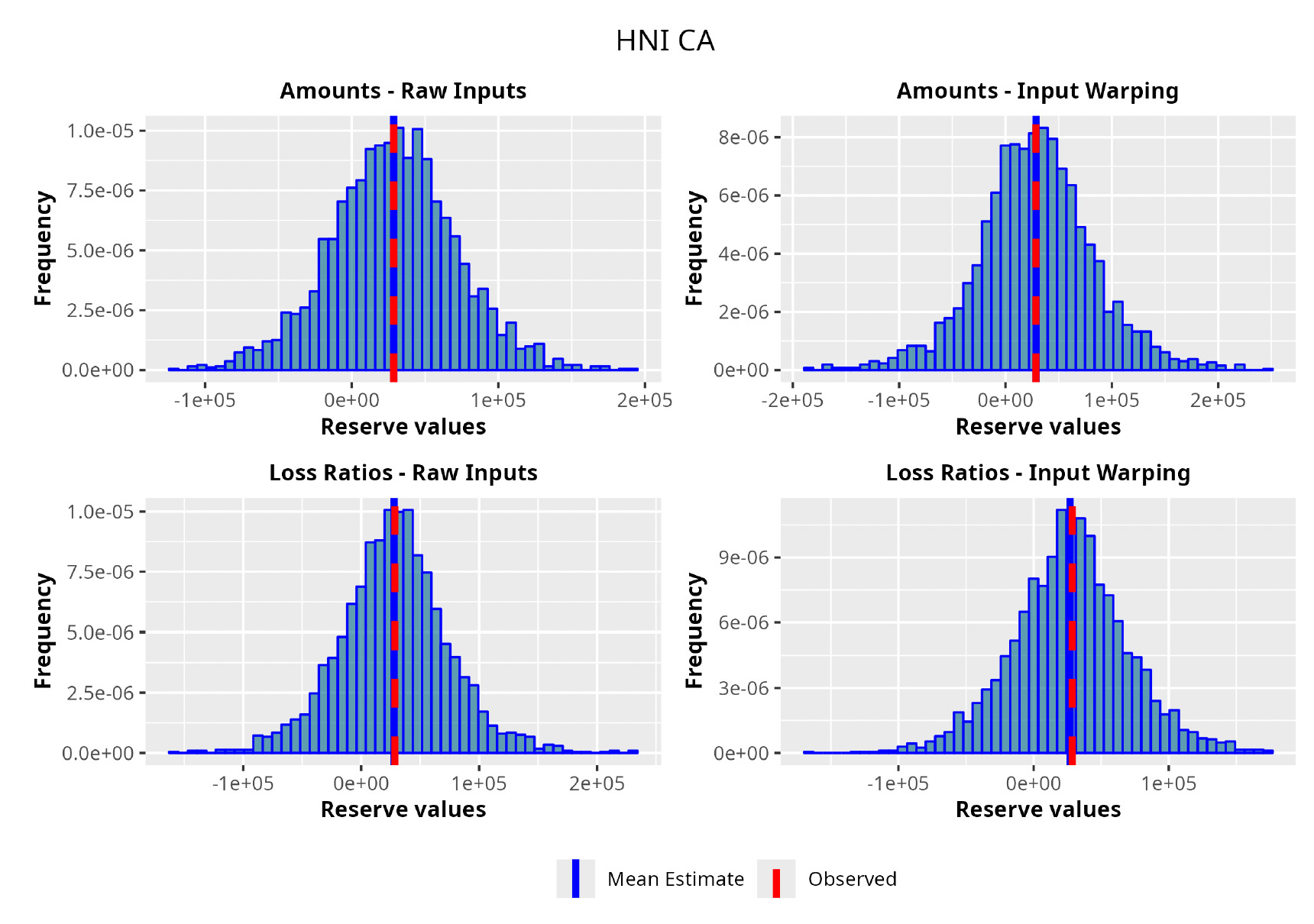
In summary, the GPR models return predictions closer to the actual ultimate loss and prove to be more adequate as risk models, providing distributions better able to capture the underlying reserve variability. Therefore, we can conclude that the GPR is a suitable Bayesian alternative to the well-established frequentist stochastic models, such as the ODP, and can be thought of as a valid option in the toolkit of the modern actuary.

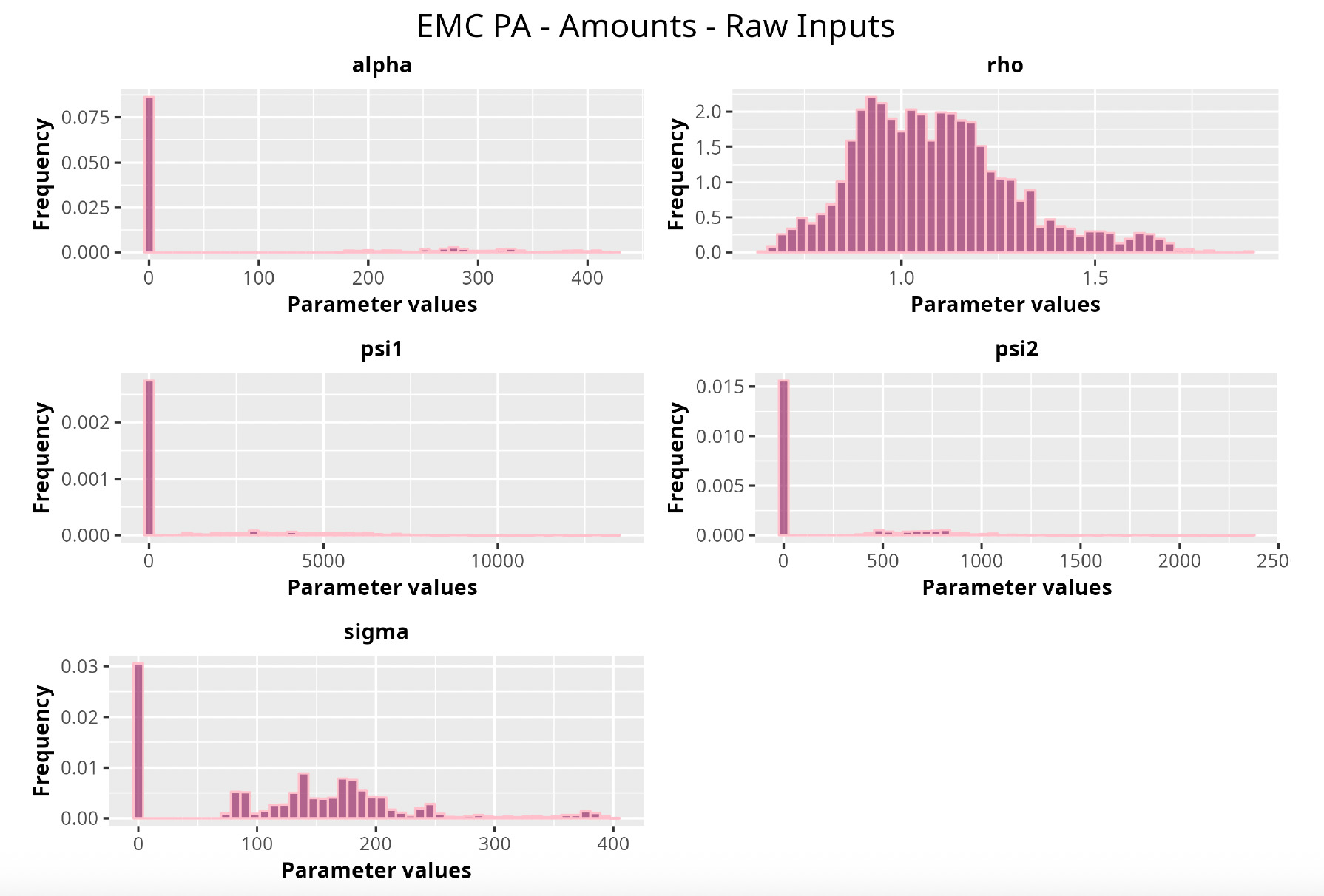
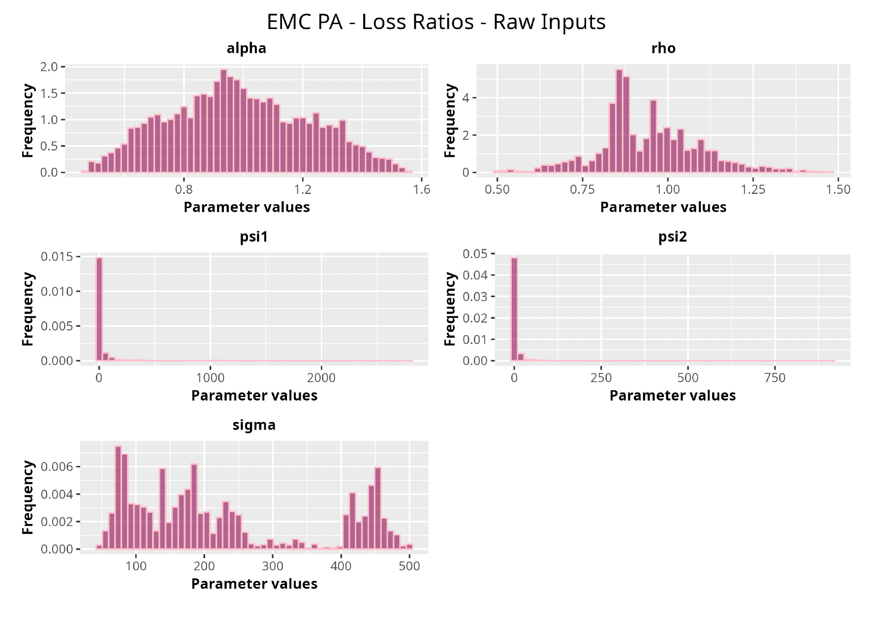
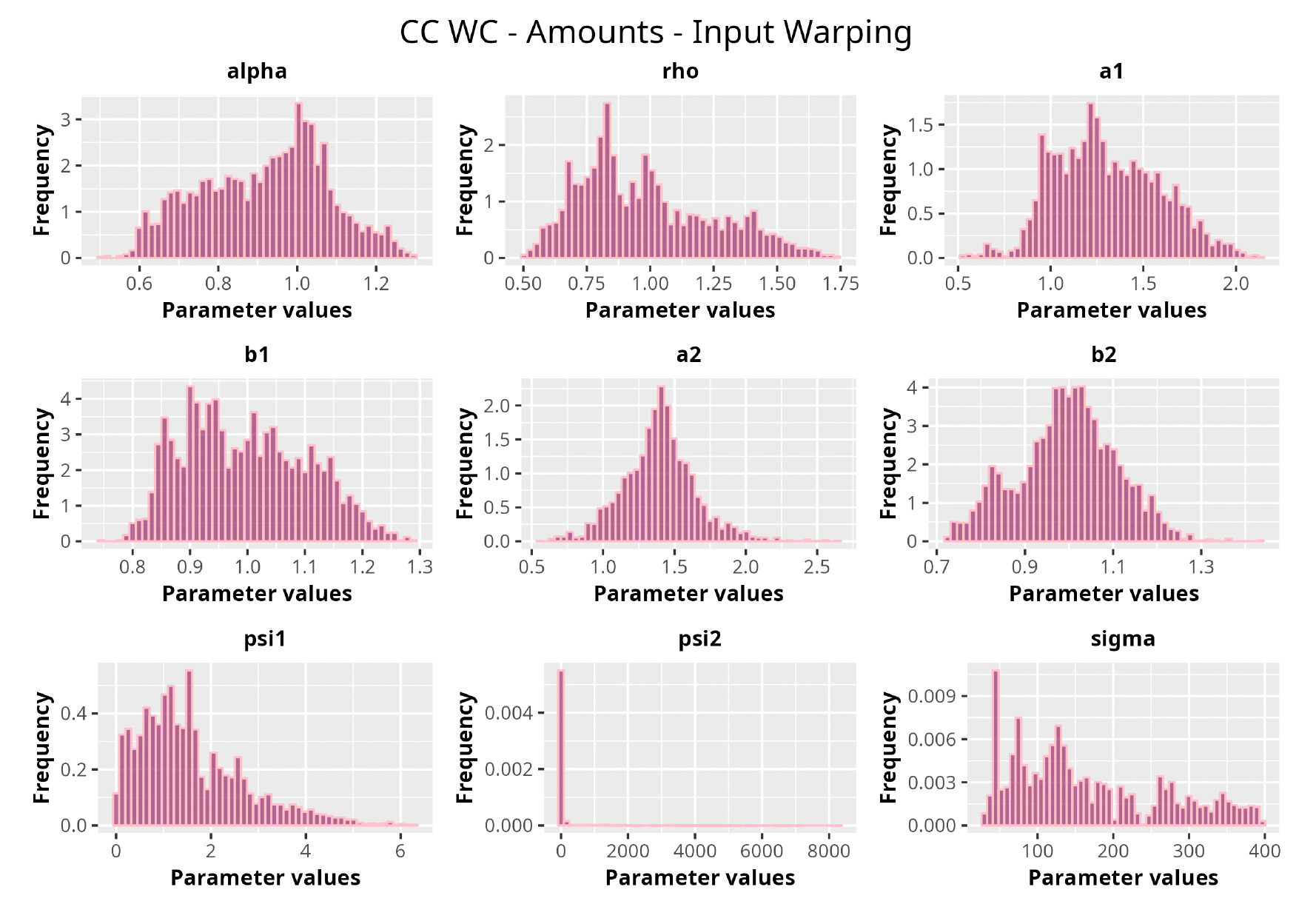
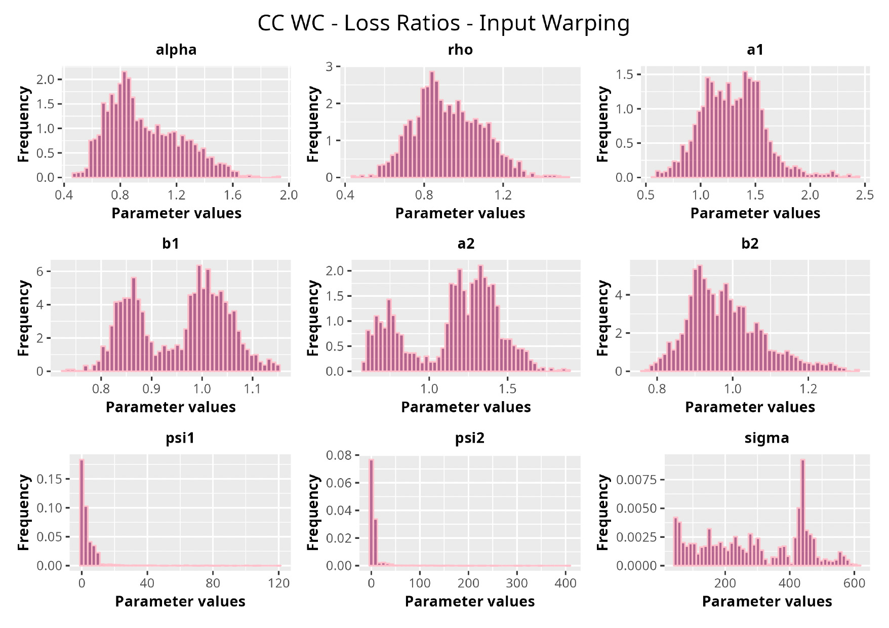
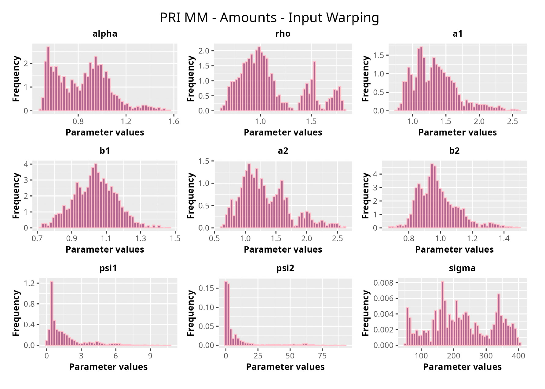
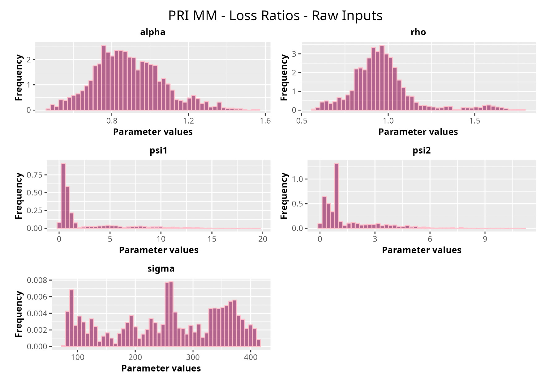
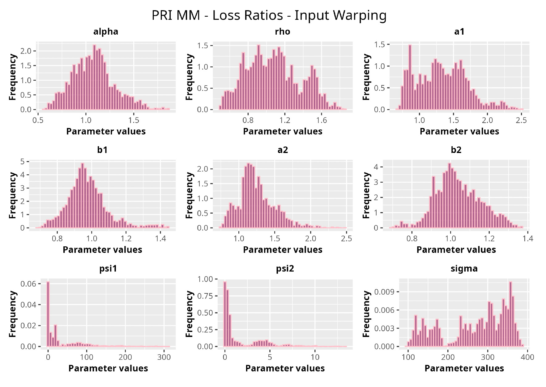
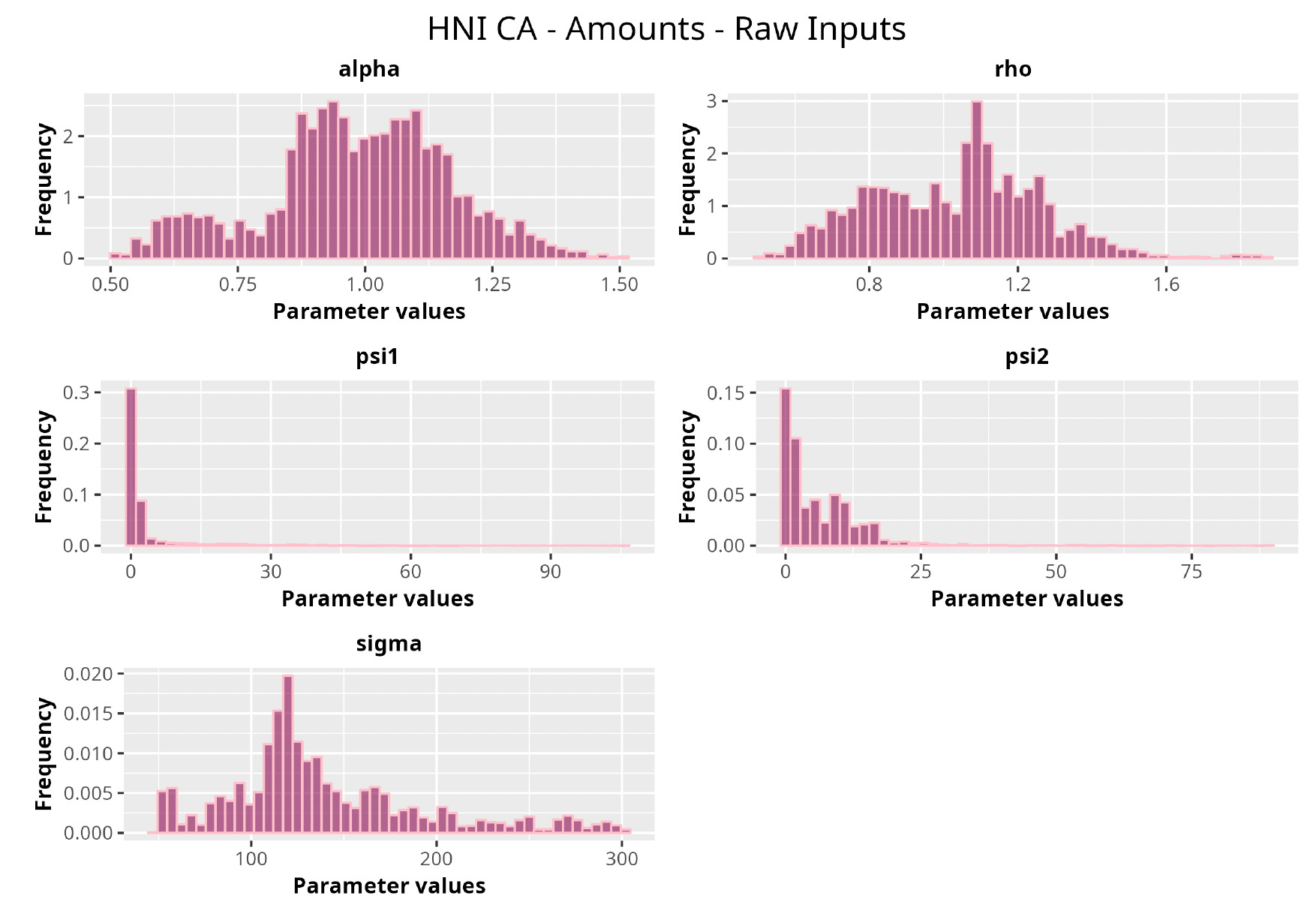
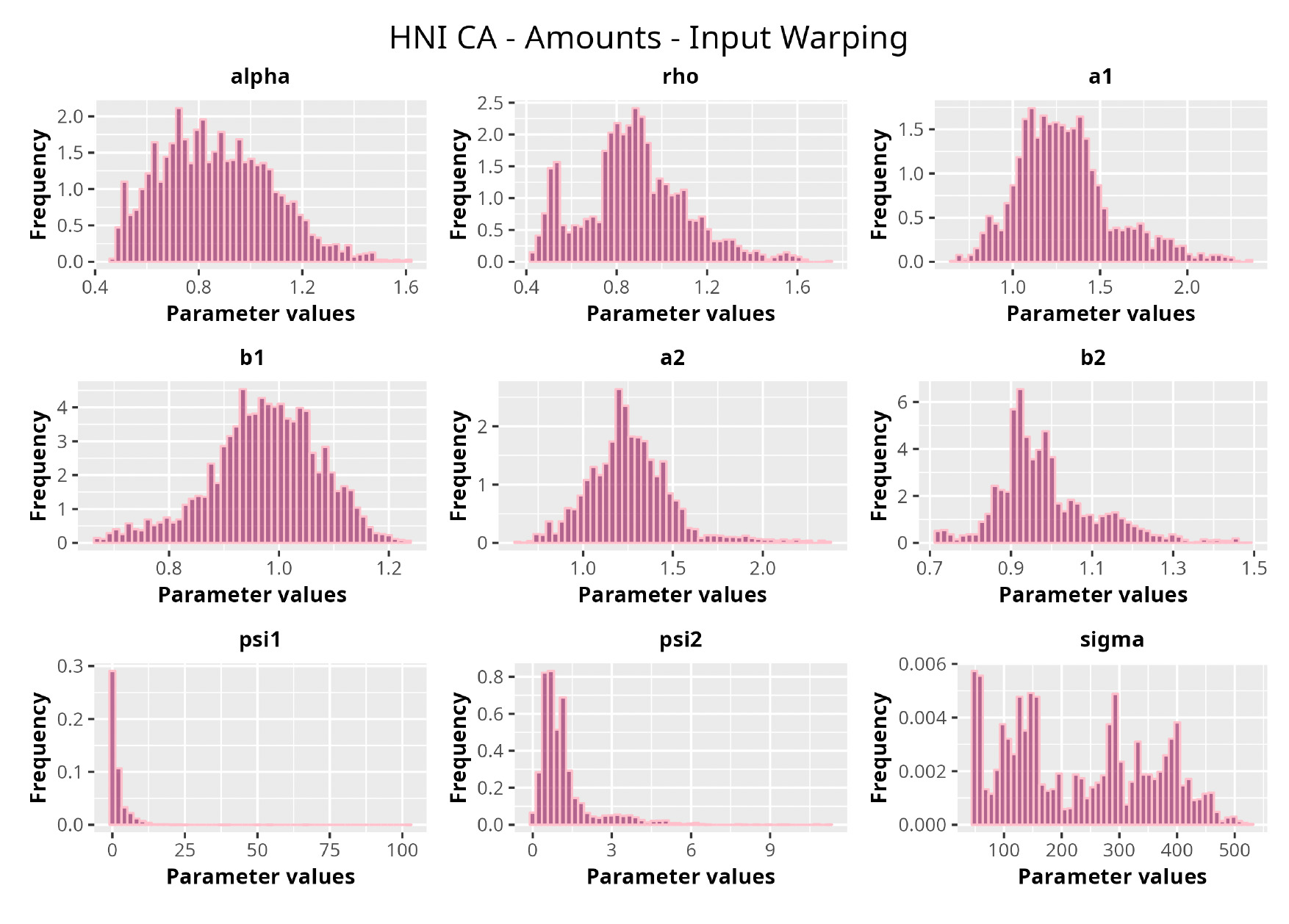
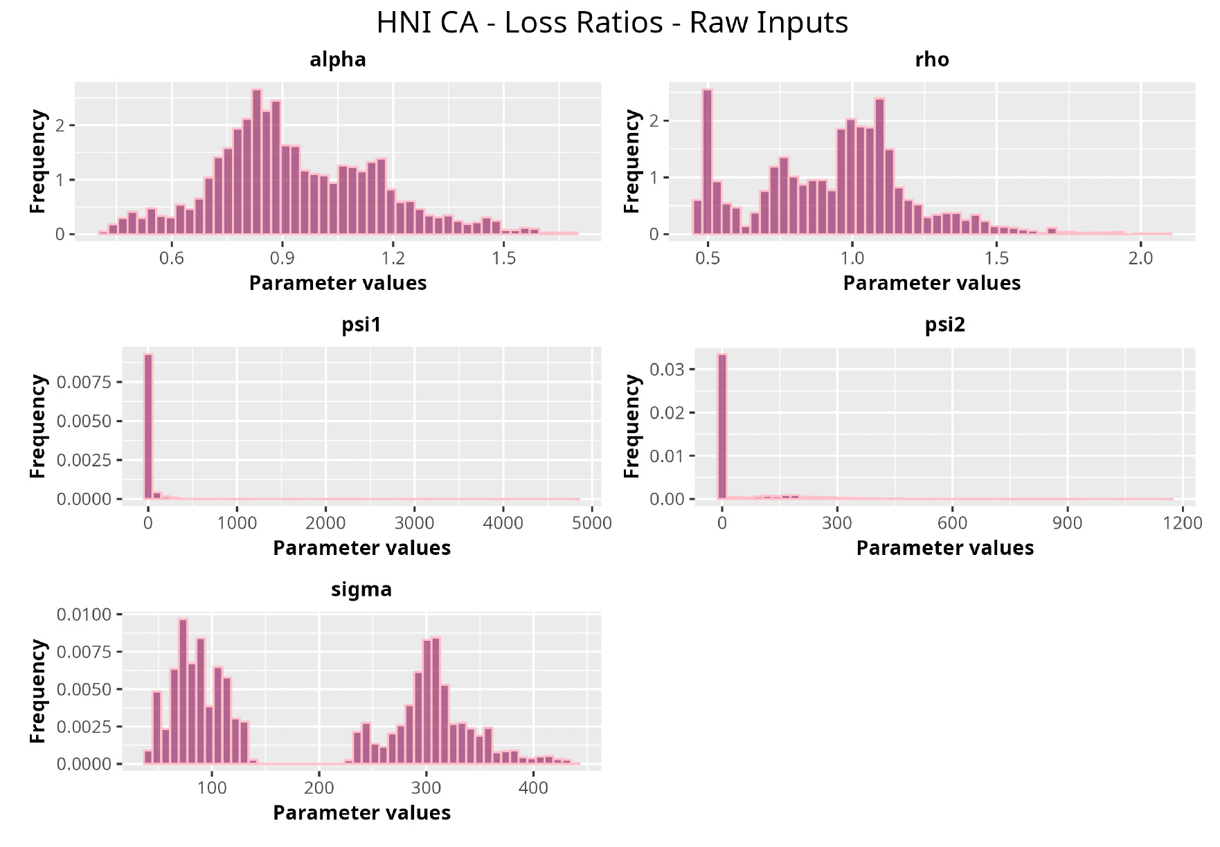
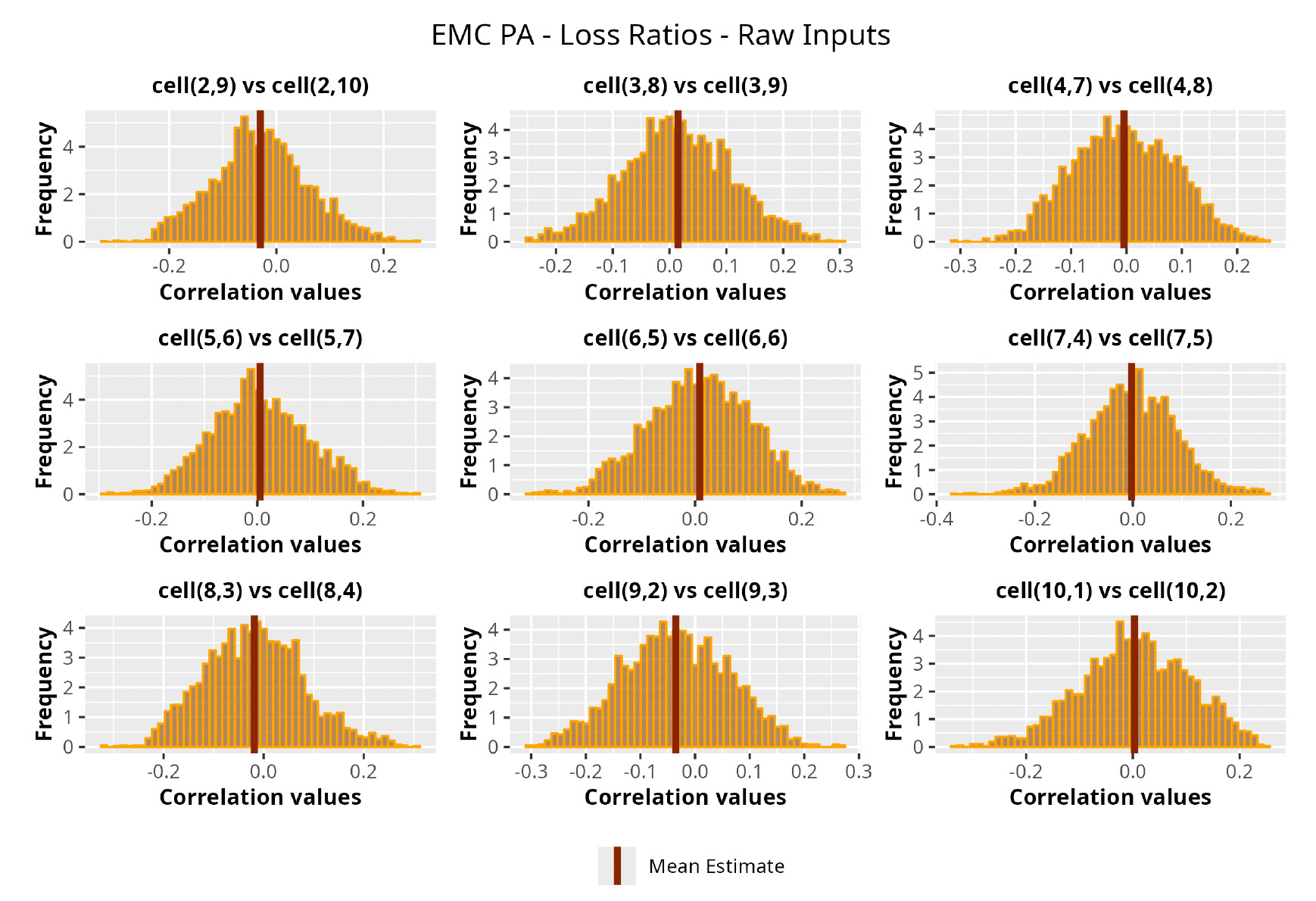
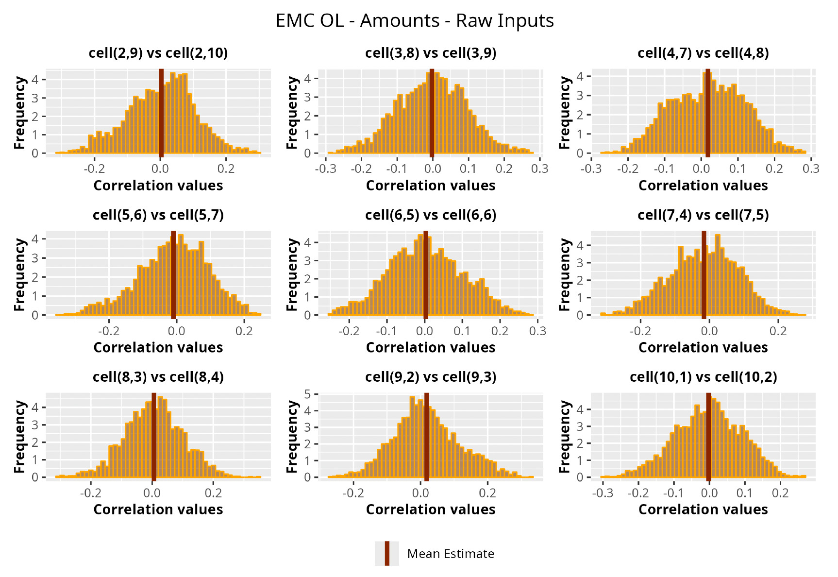
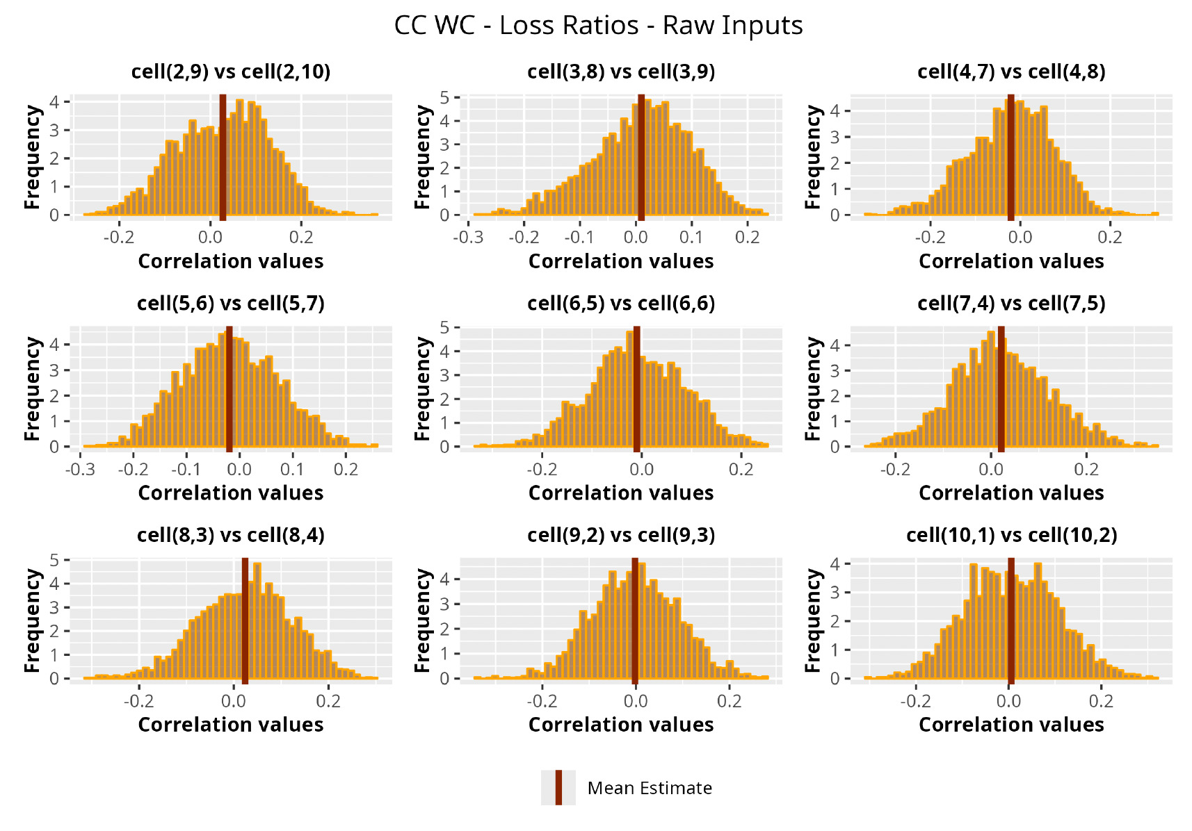
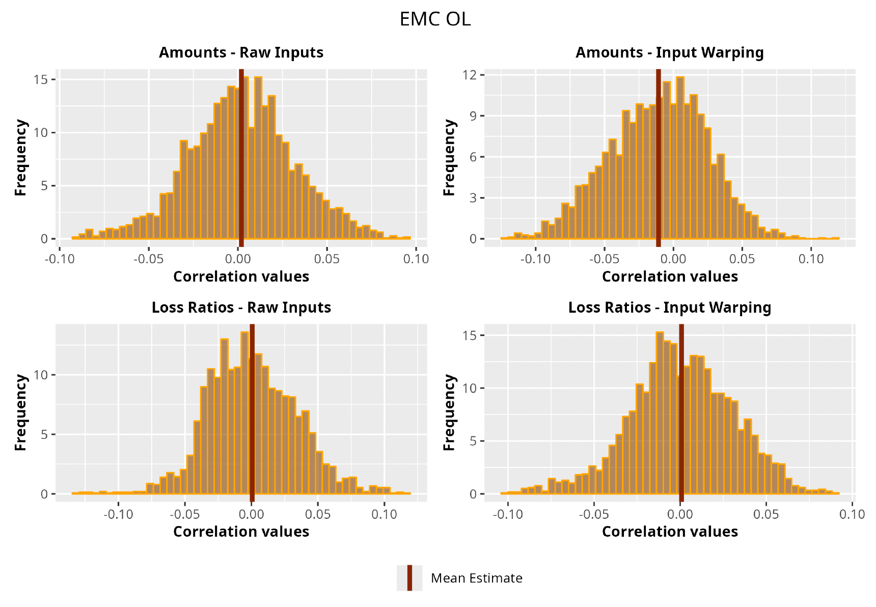
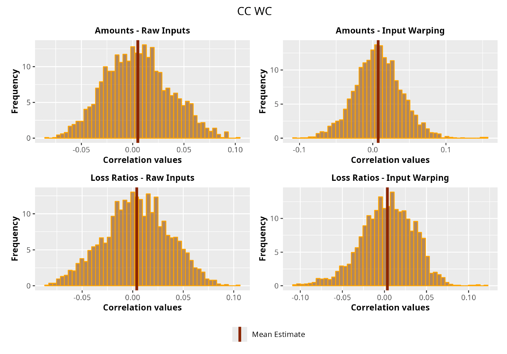
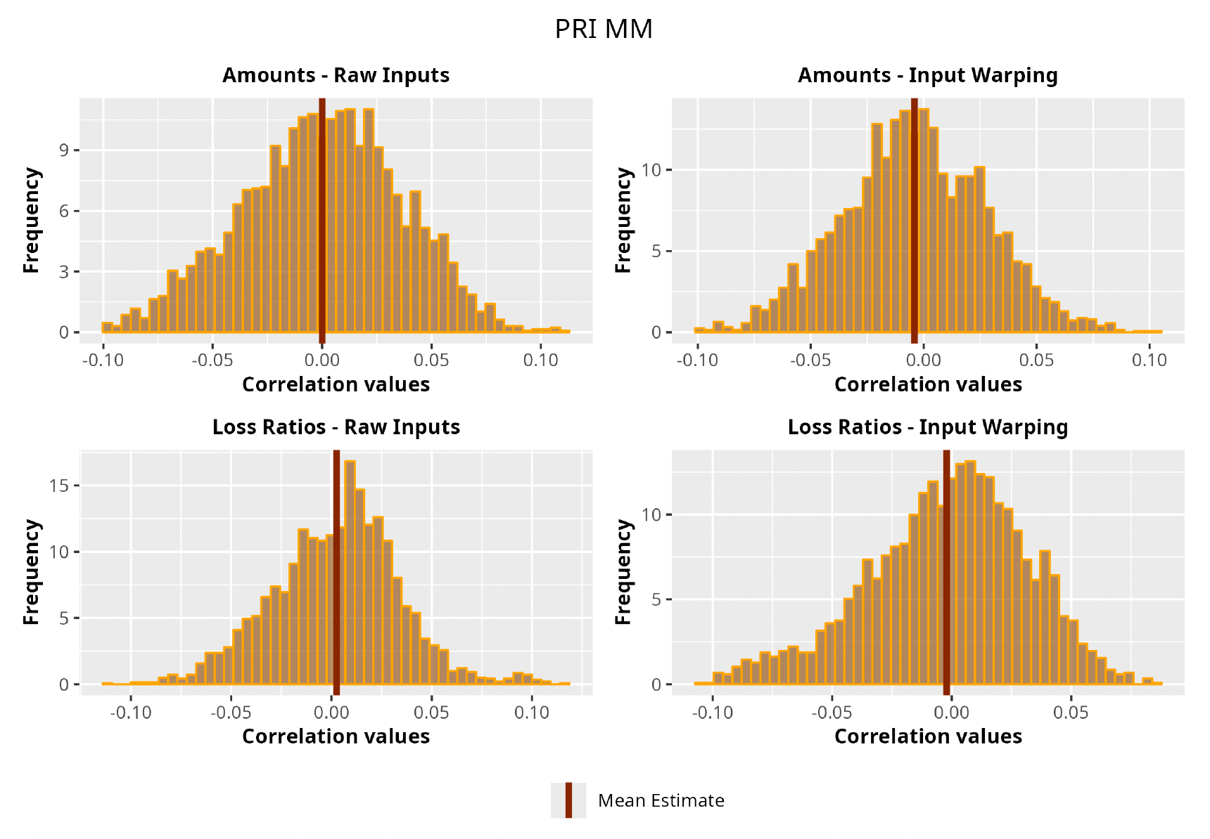
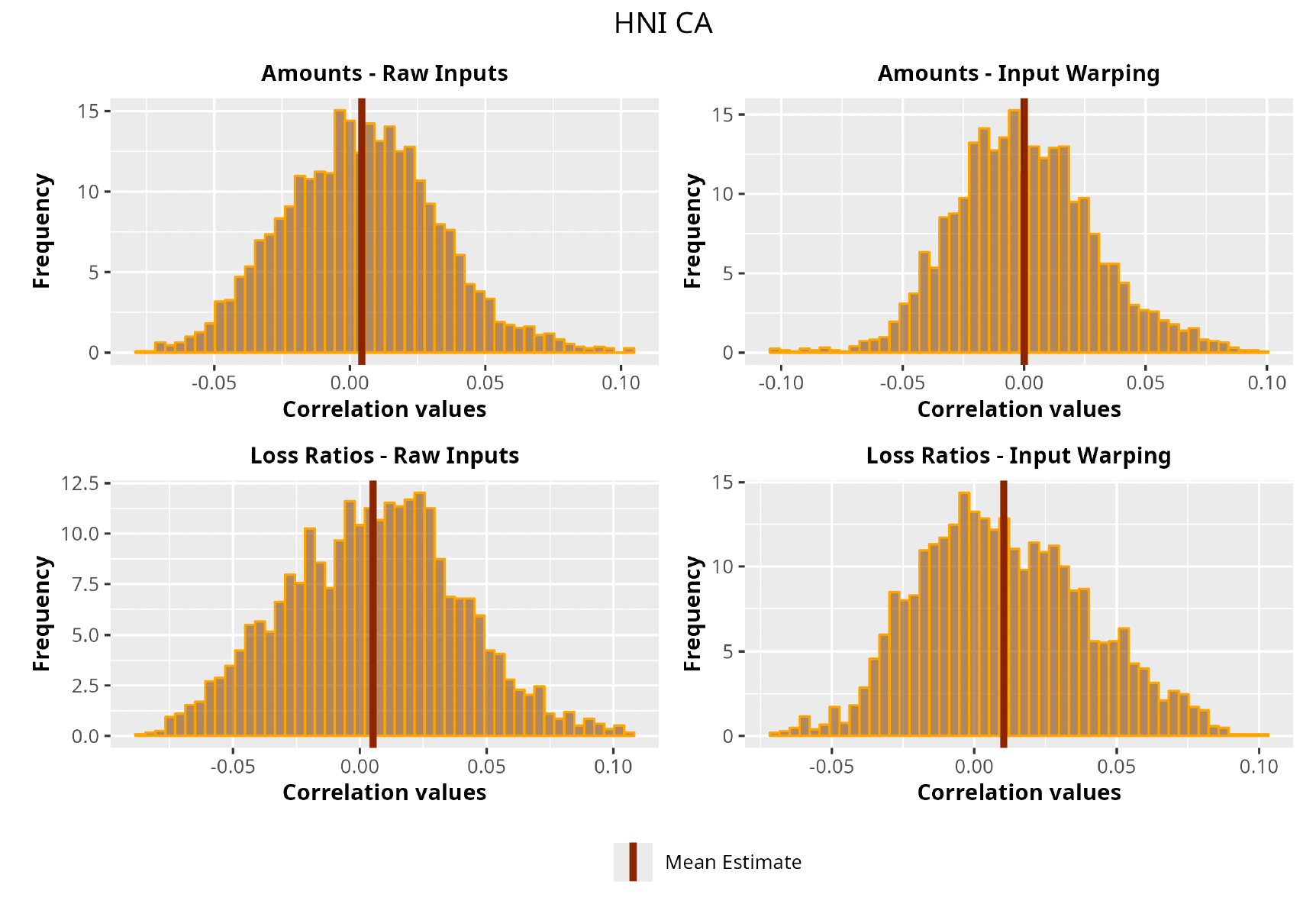
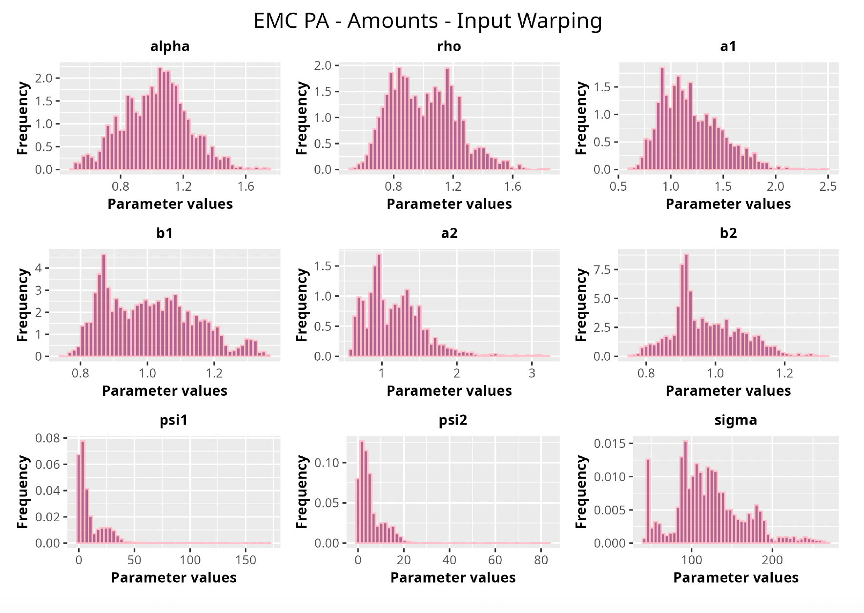
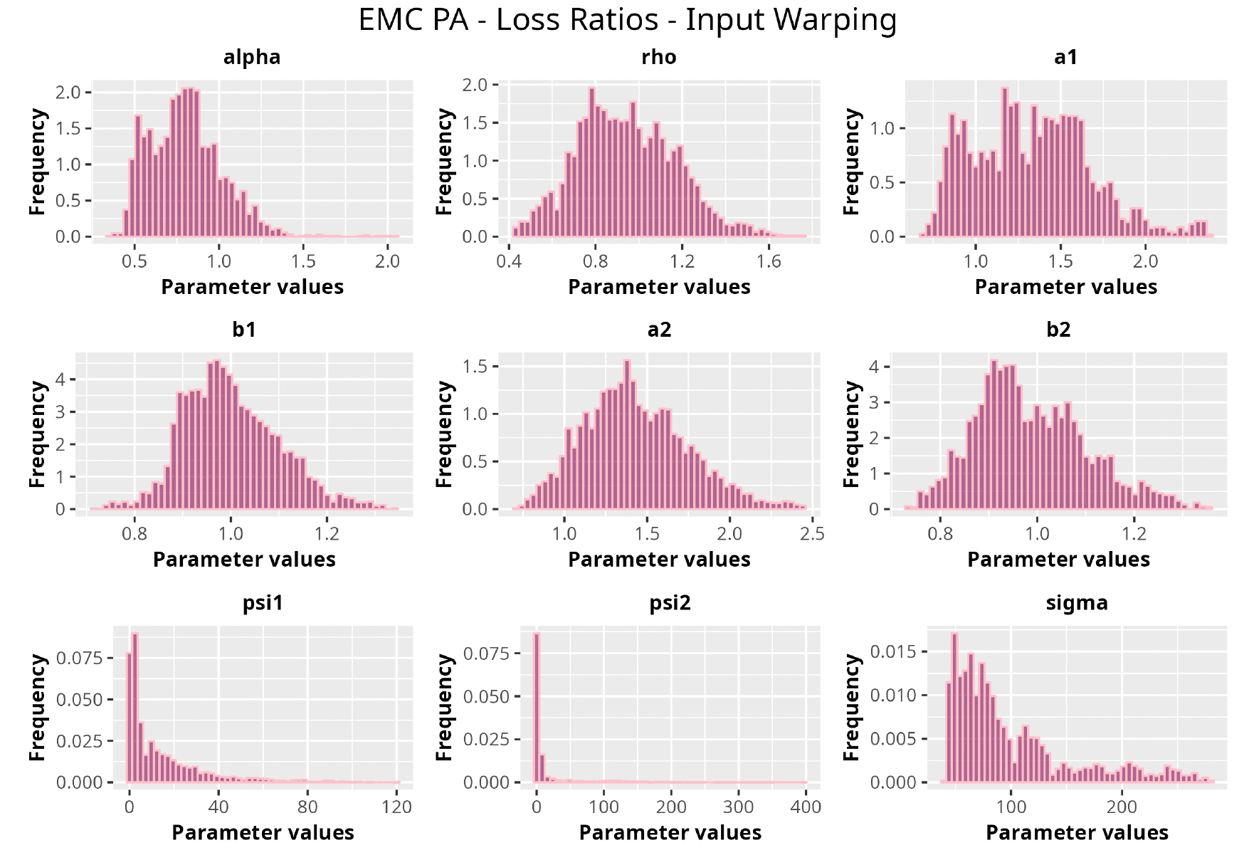
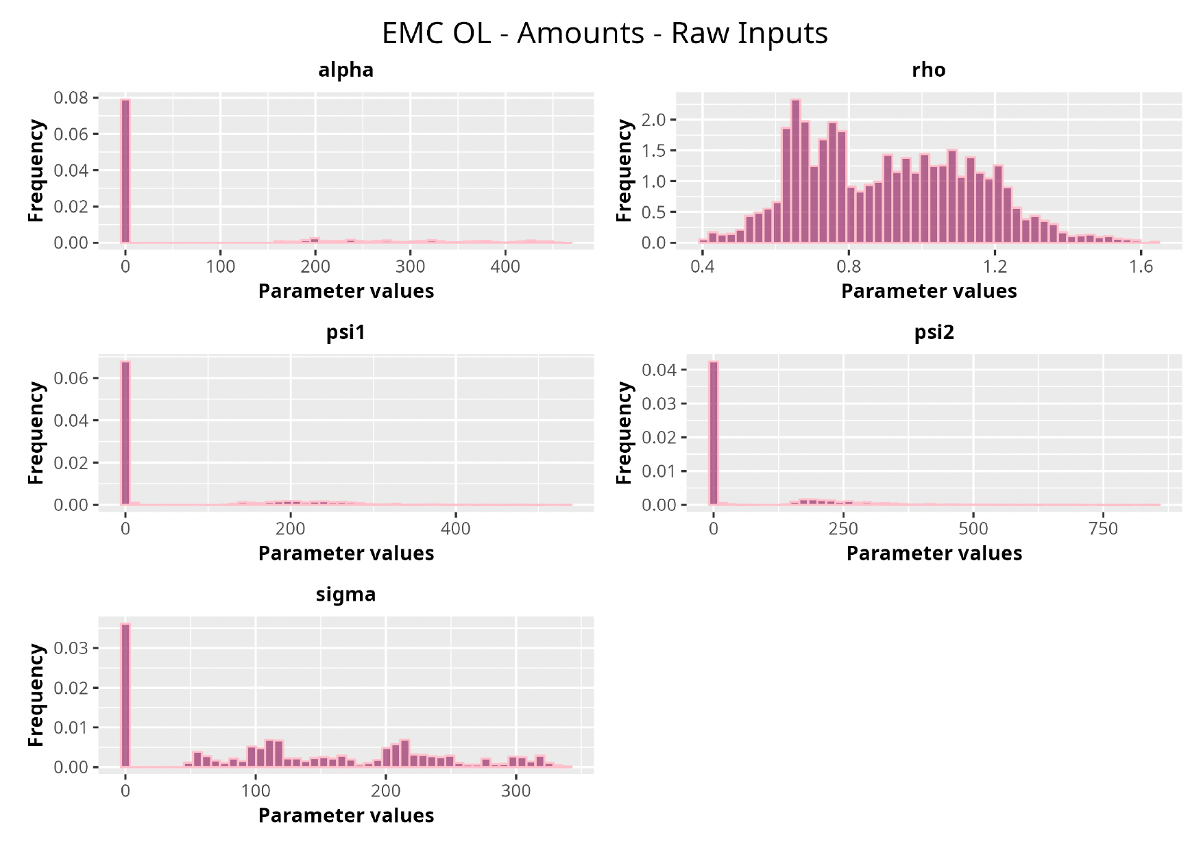
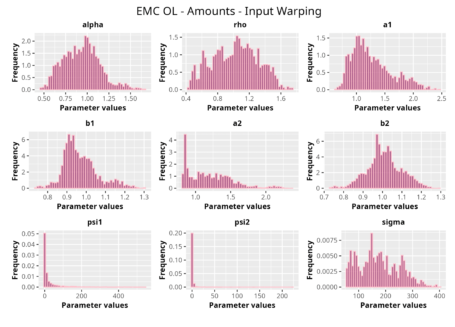
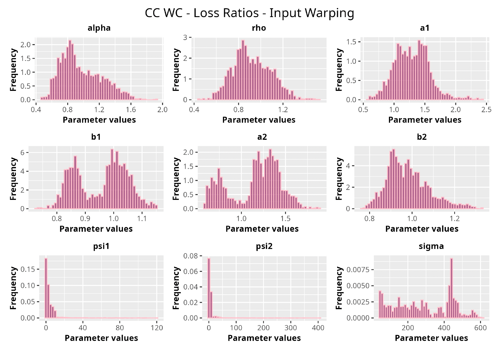
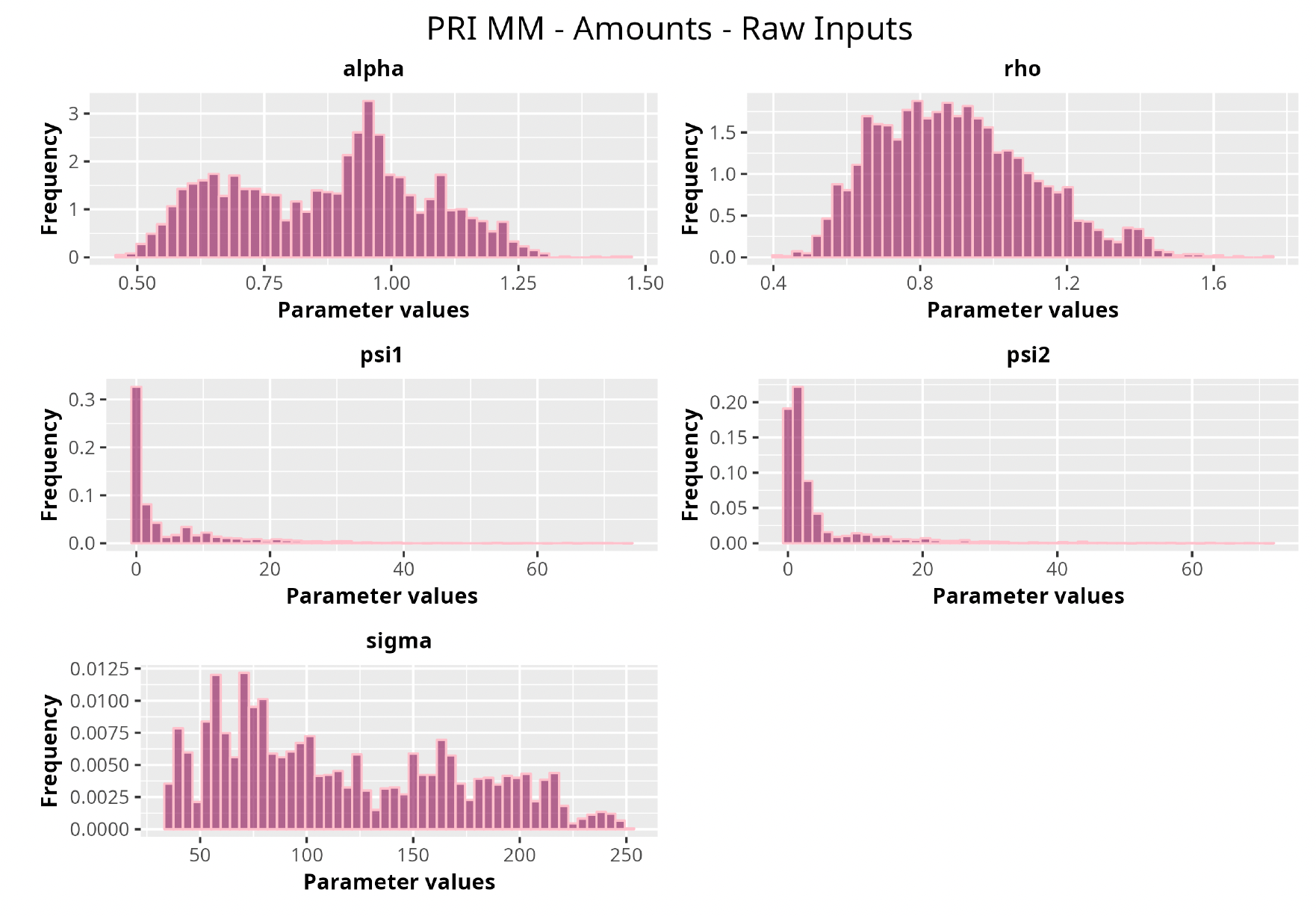
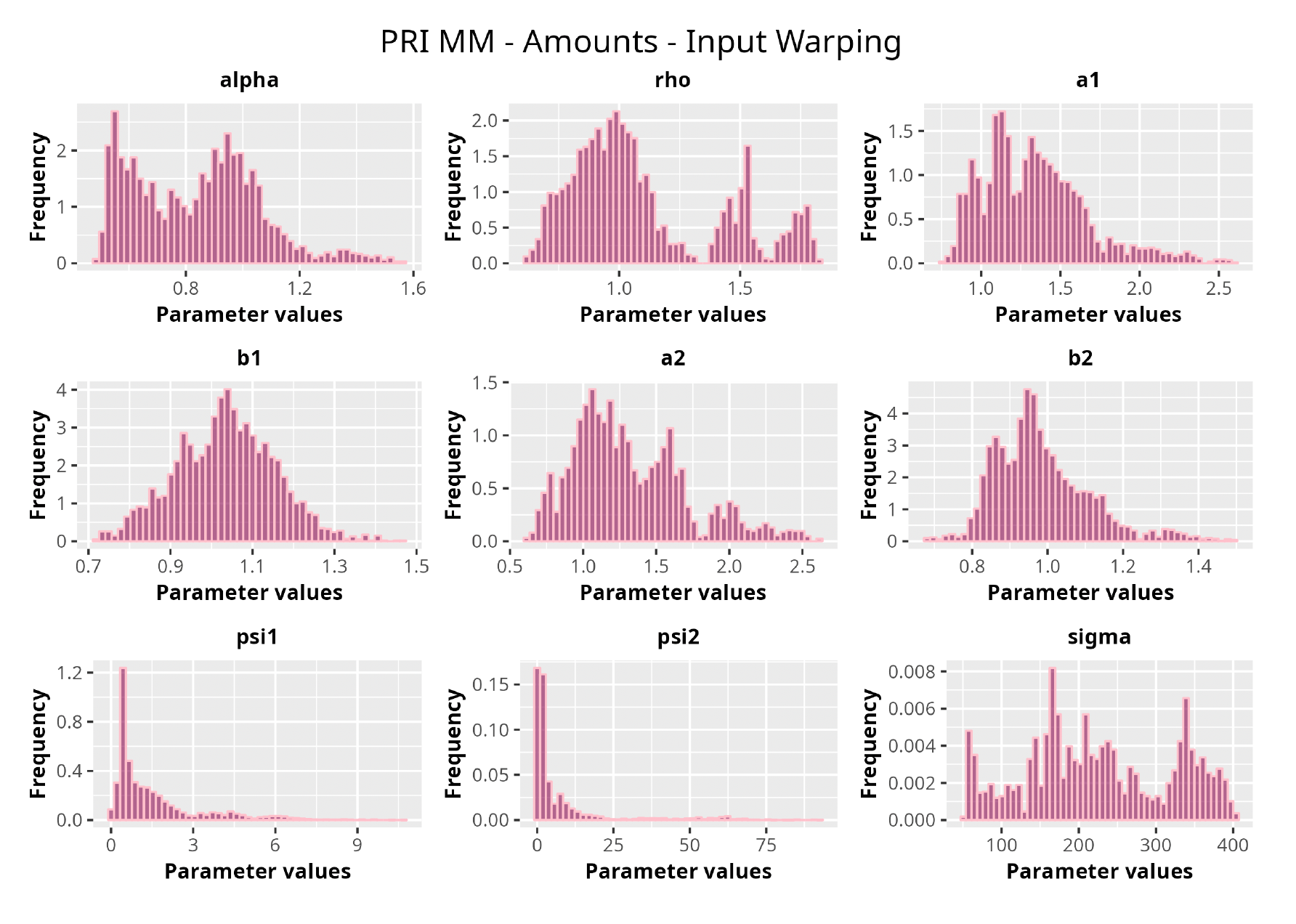
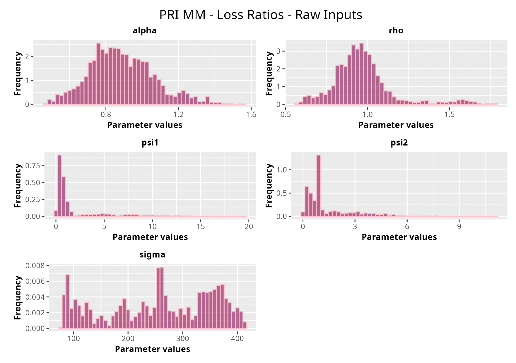
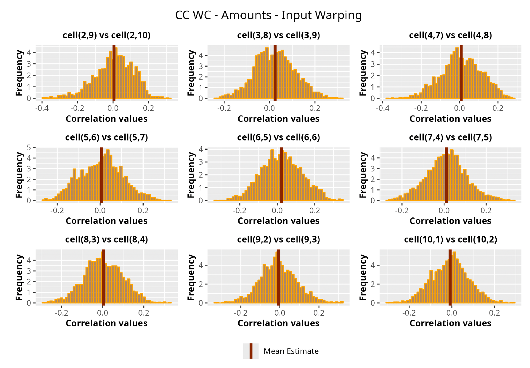
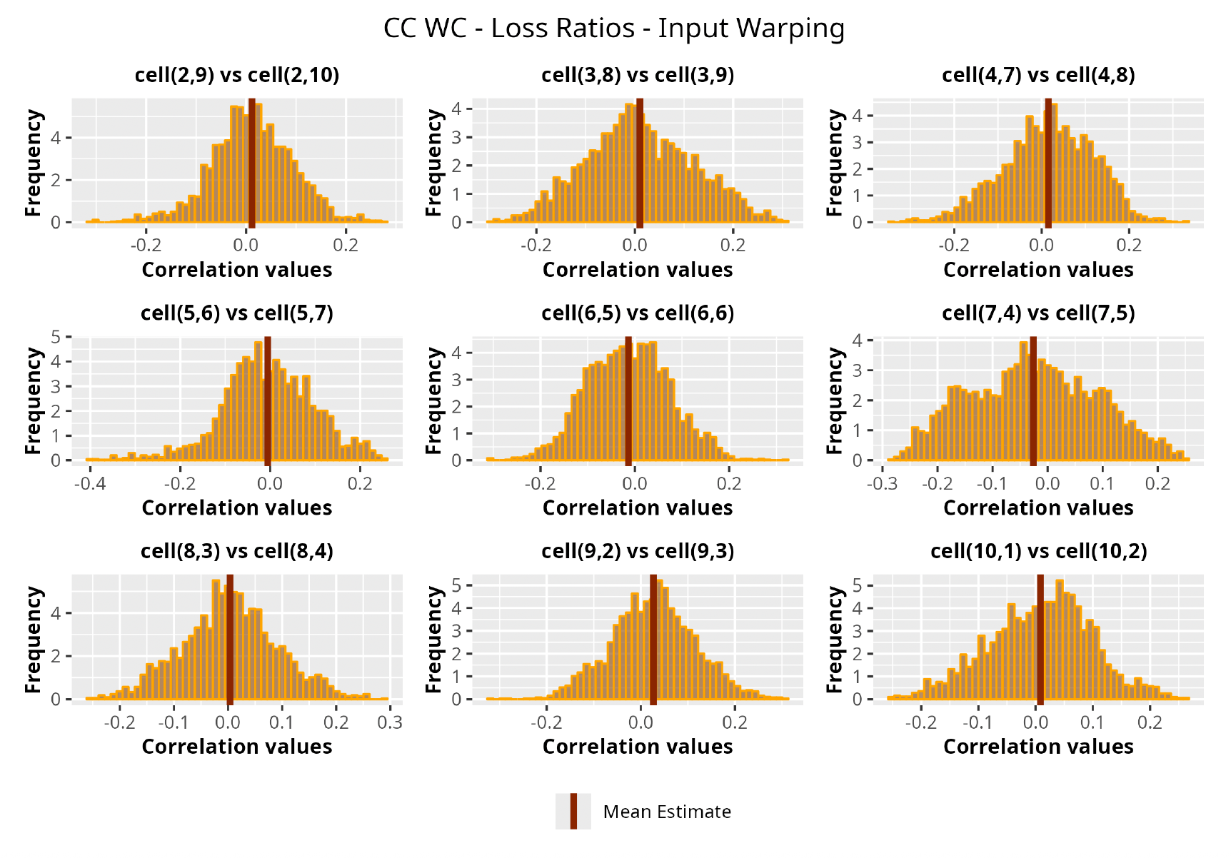
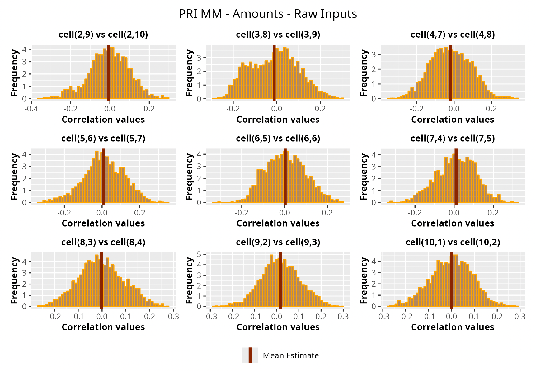
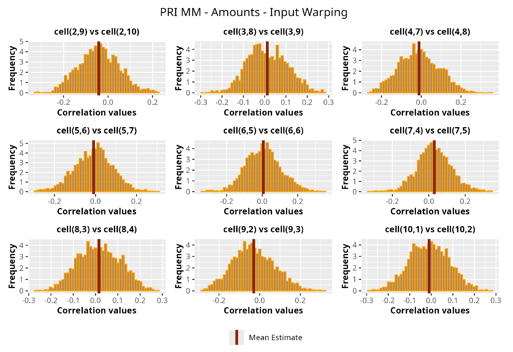
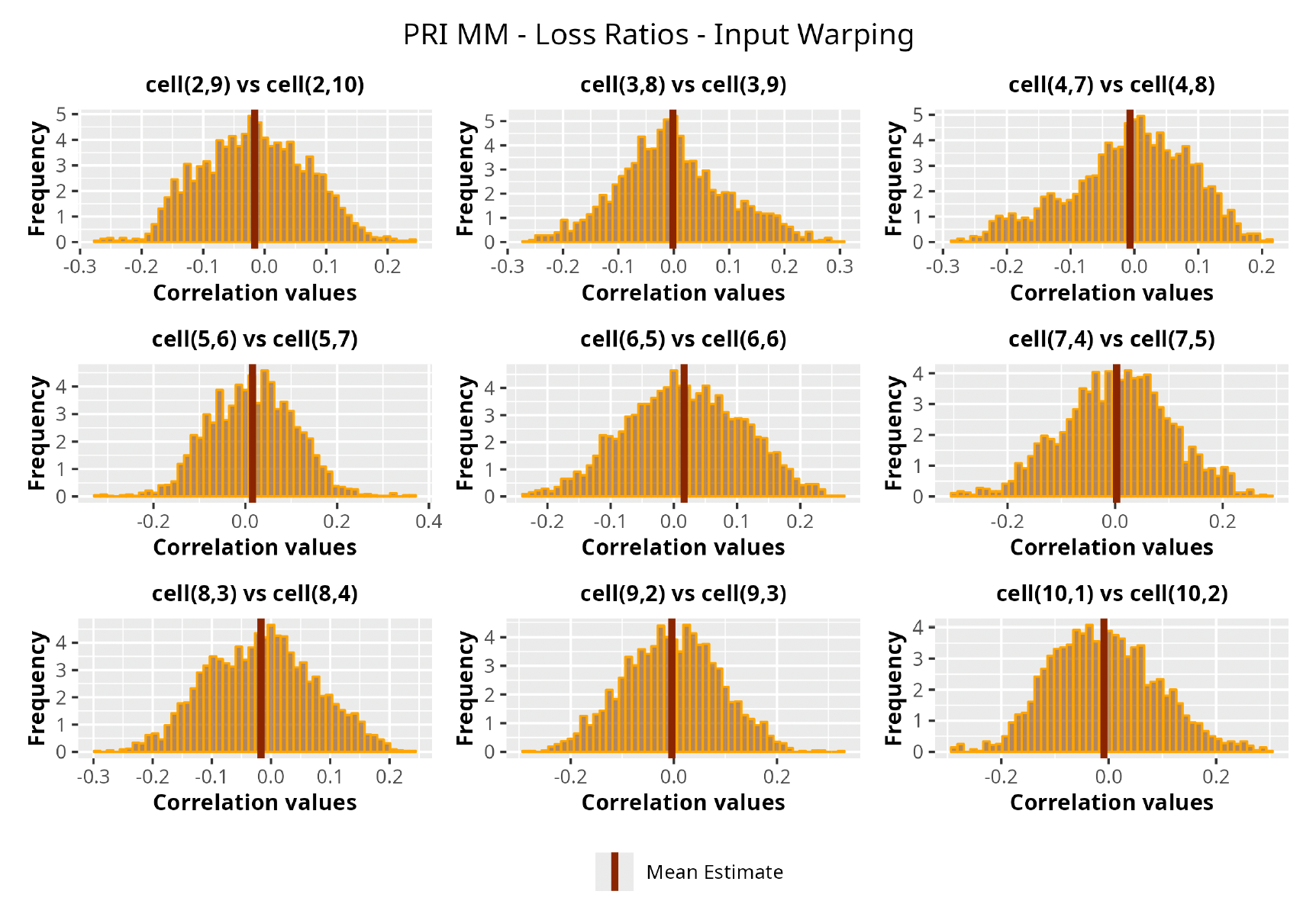
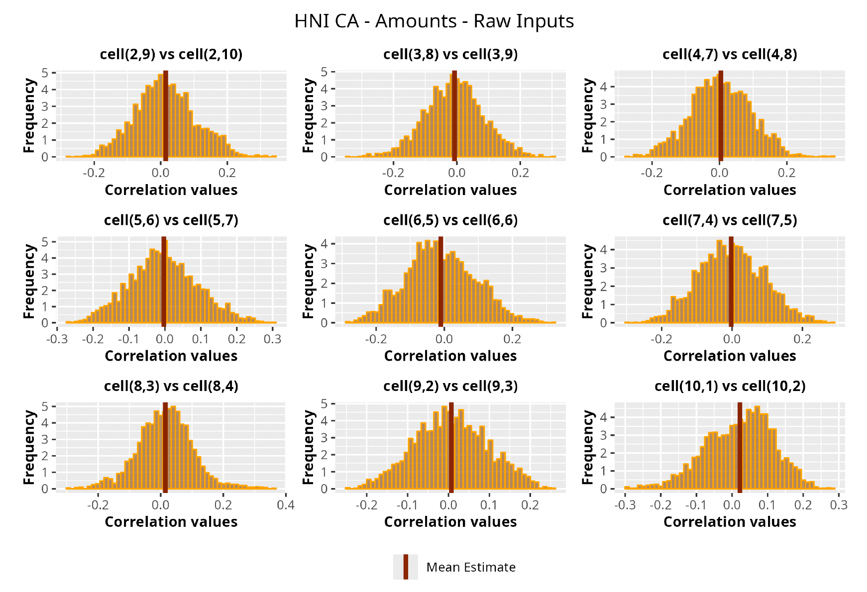
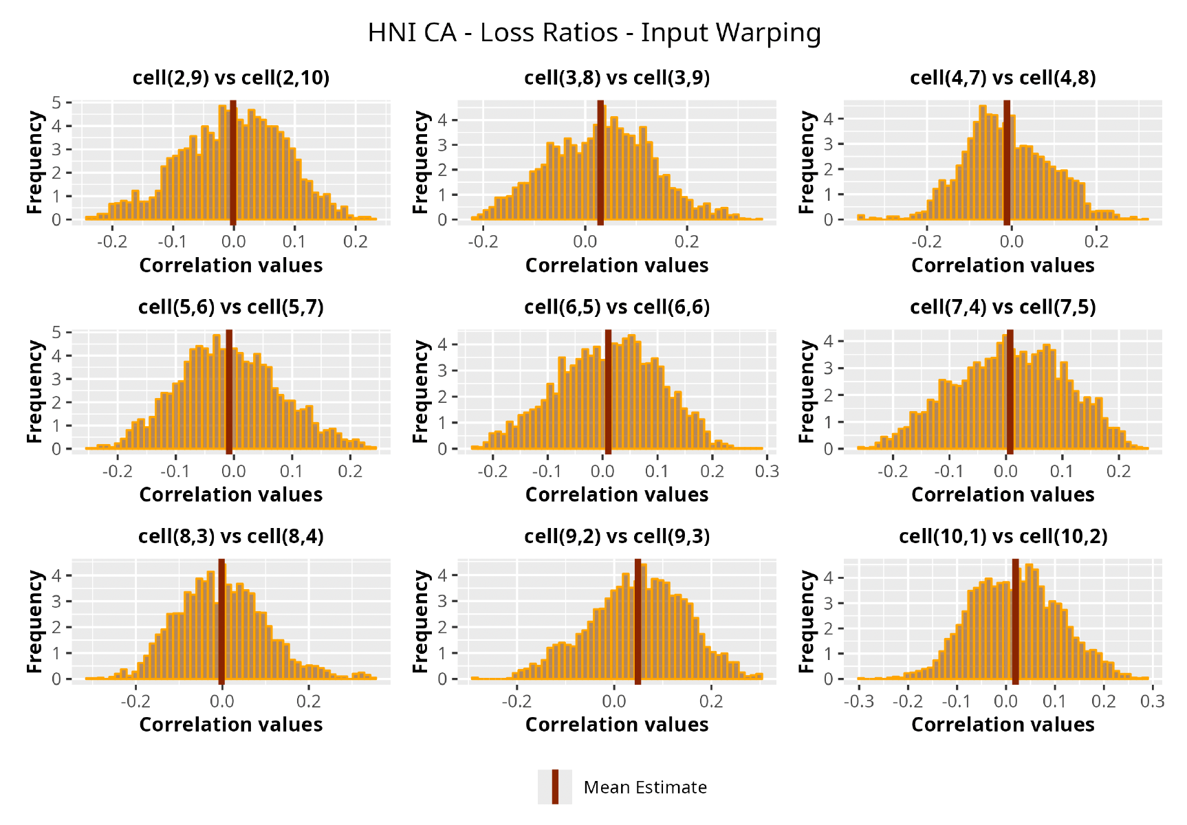
7.1. Correlation analysis

This section is dedicated to the analysis of the correlation matrices^[13] that define the GPR models implemented.

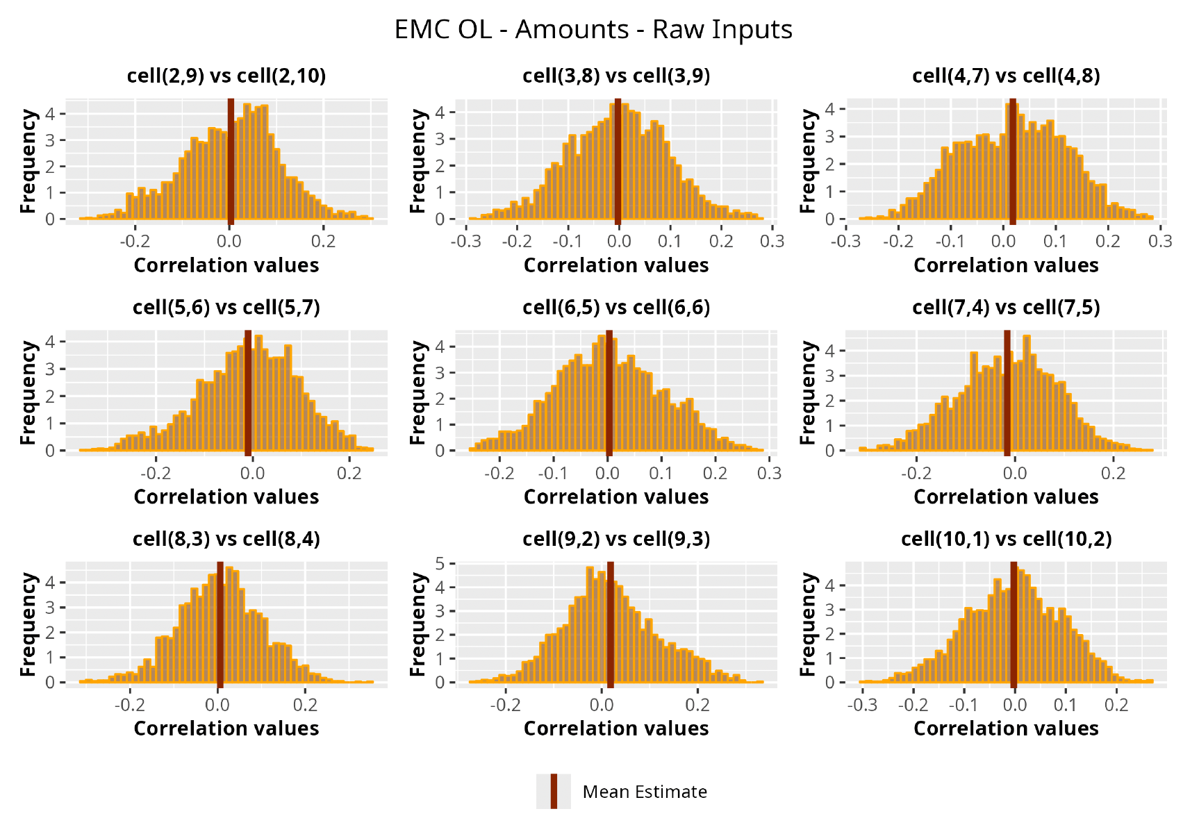
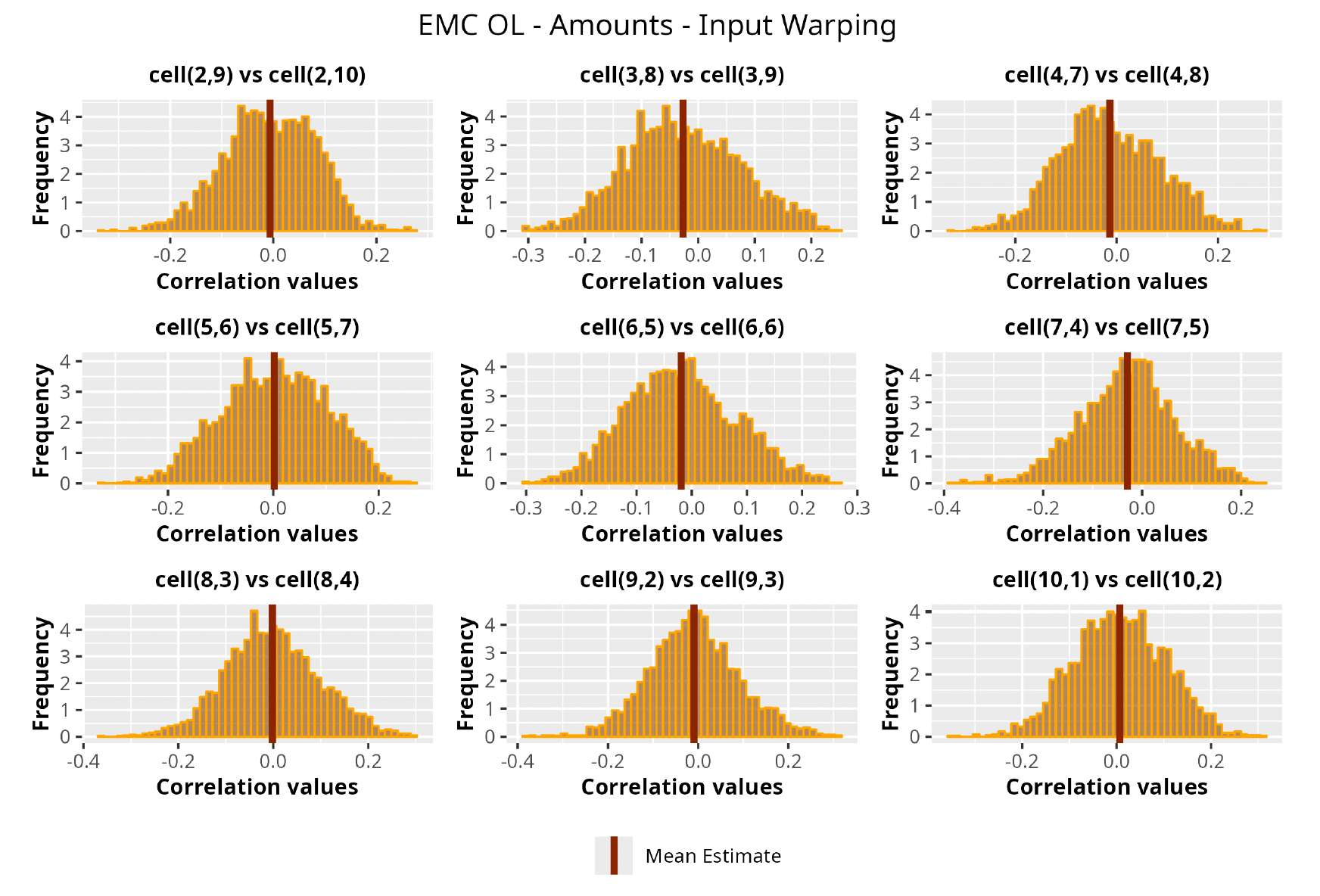
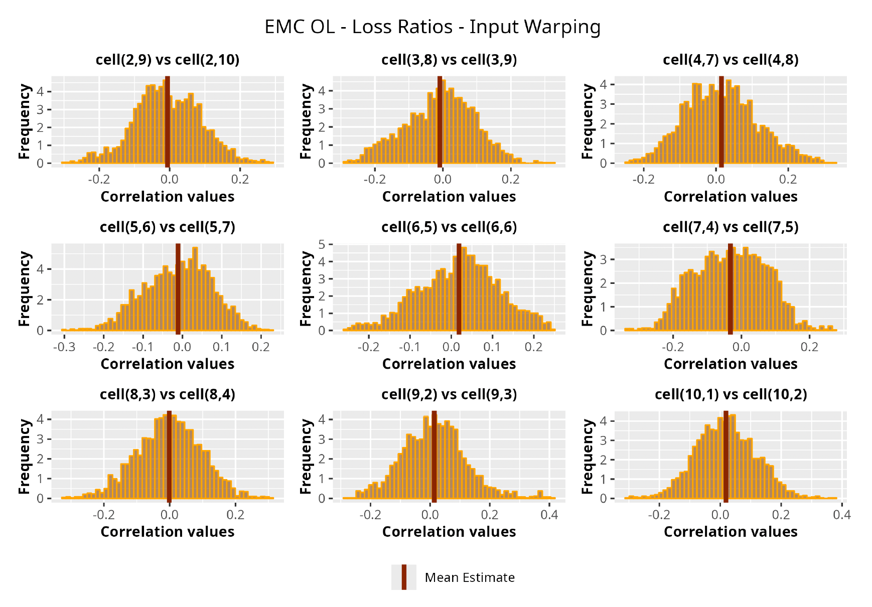
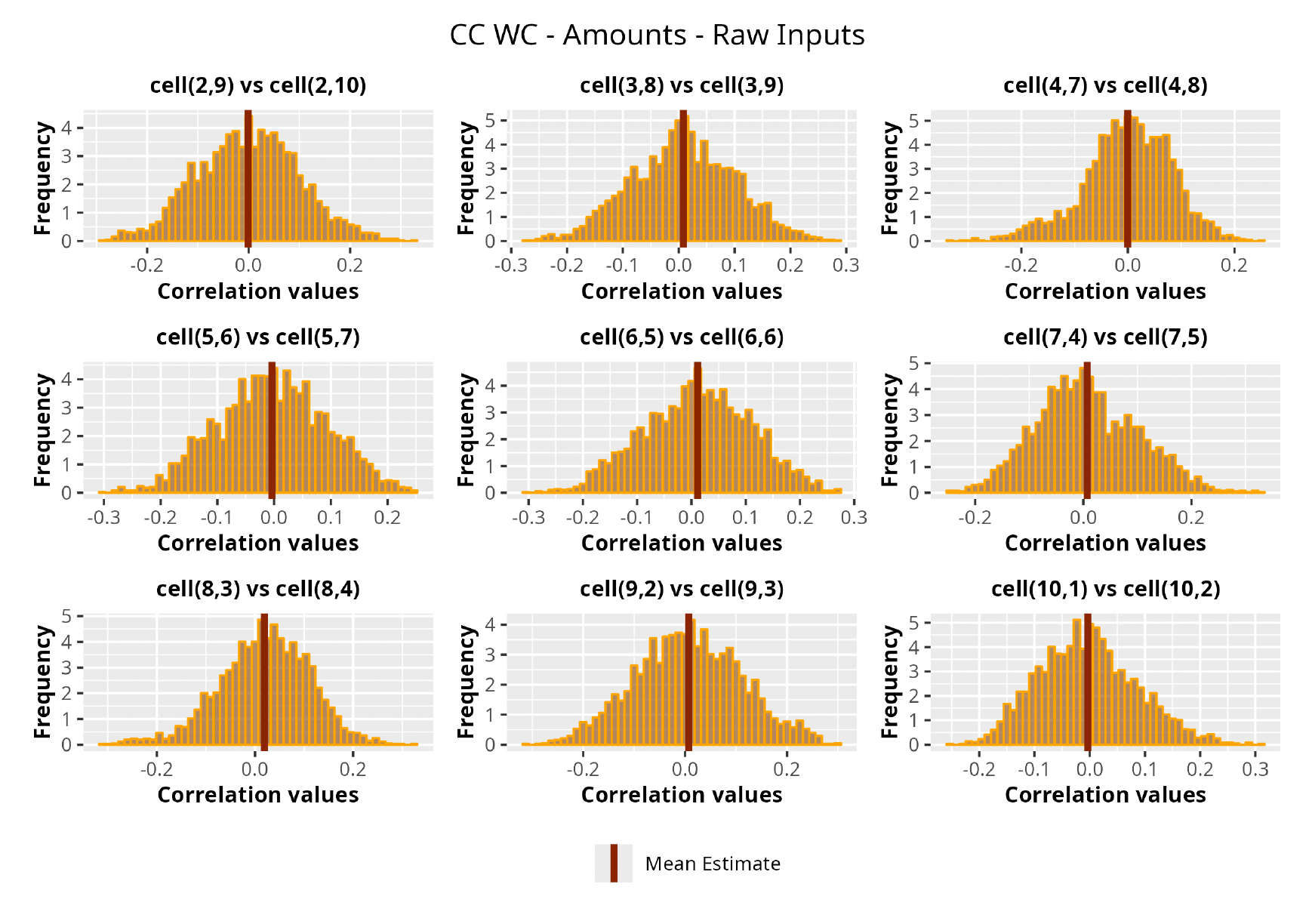
The procedure described in the previous sections models the posterior distribution of the covariance between all the pairwise combinations of the cells in the claims triangle as an inverse Wishart distribution. Analyzing the behavior of this stochastic matrix will give us more insight into how claims develop and, more important, whether any significant correlations exist between payments. This procedure could be useful for a variety of reasons—from claims reserving to setting capital requirements.

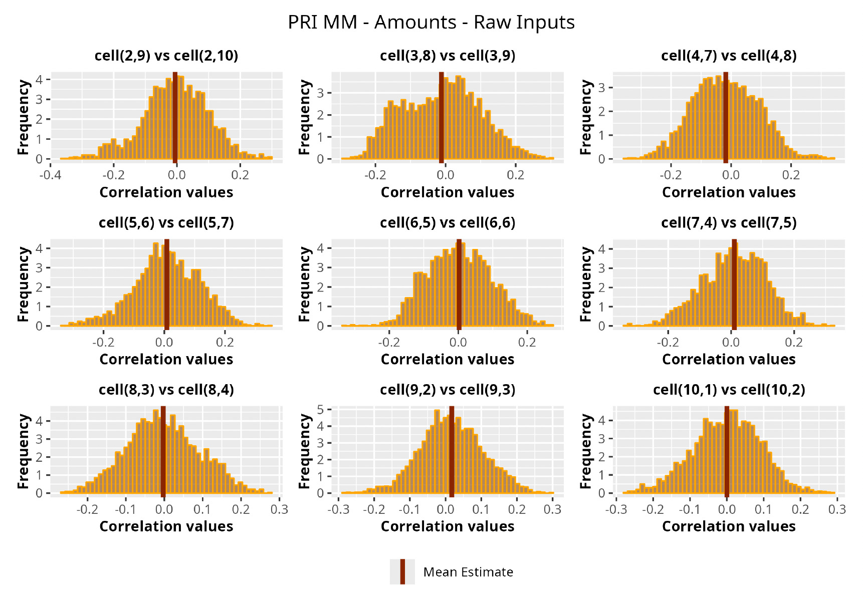
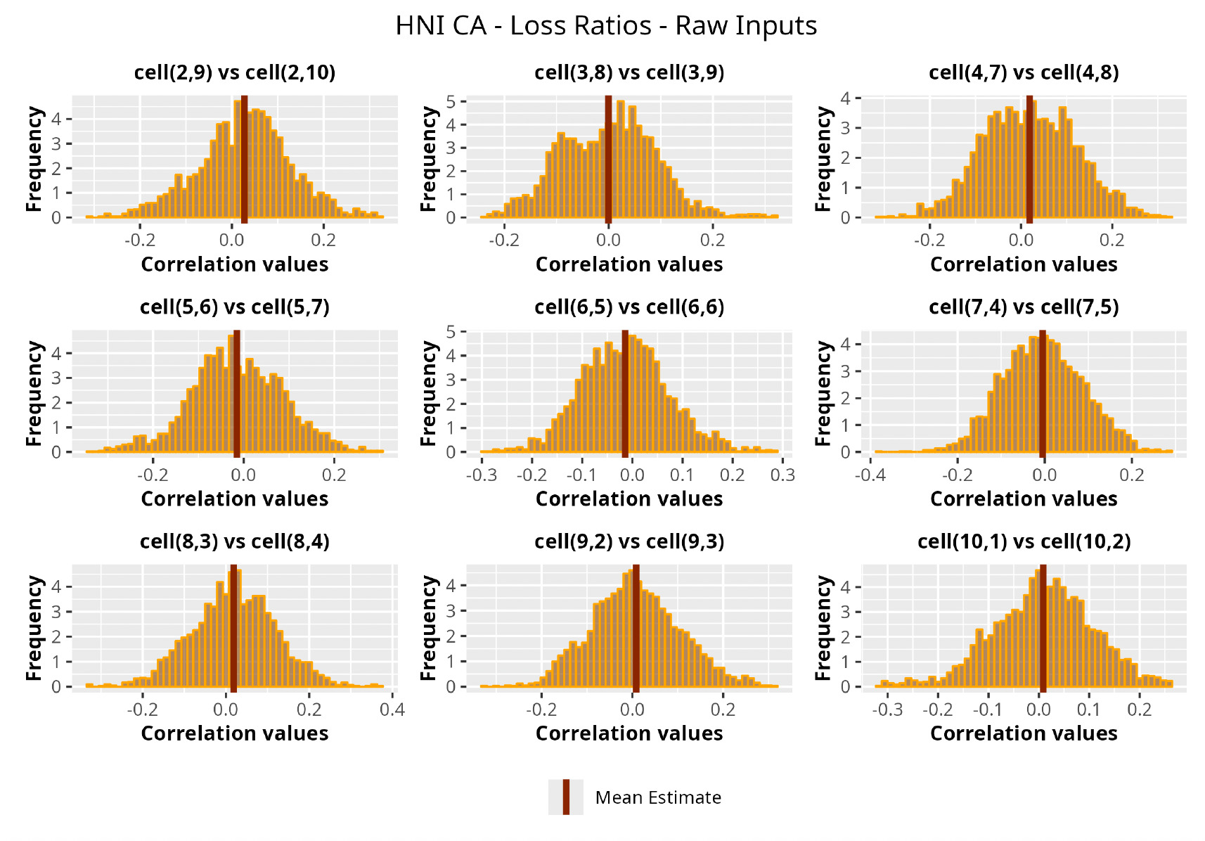
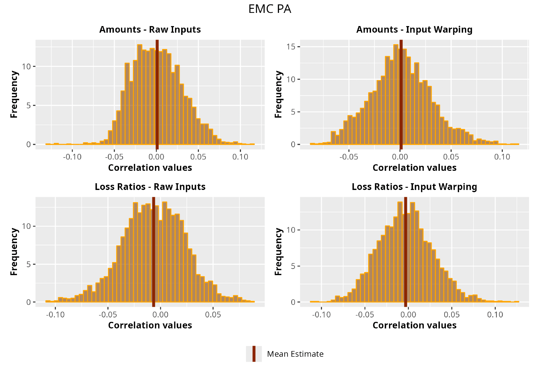
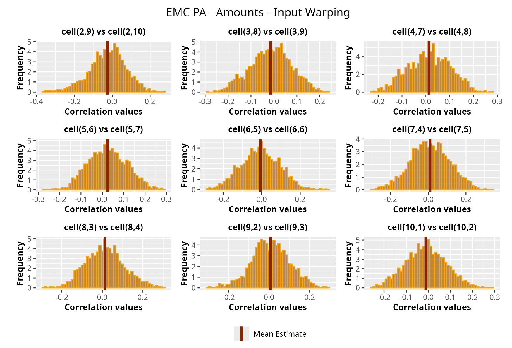
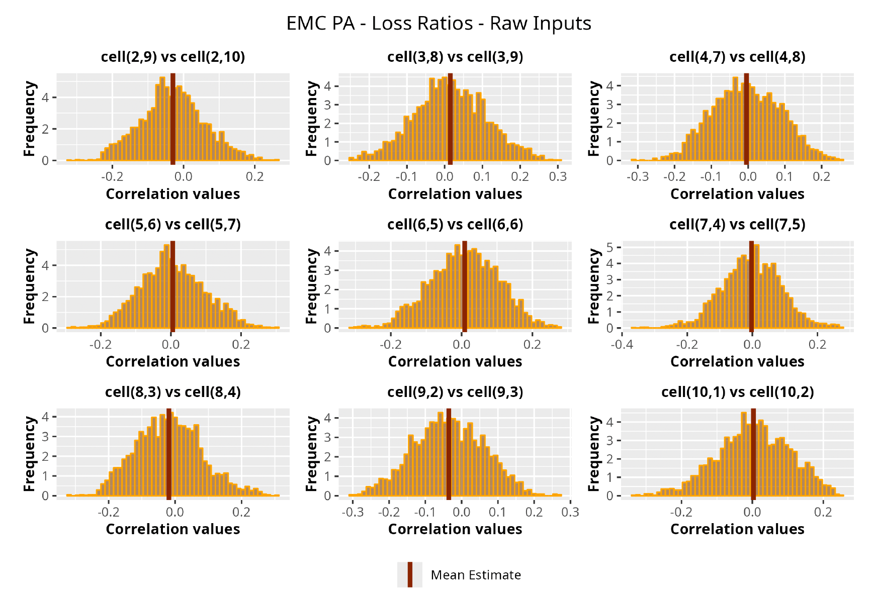
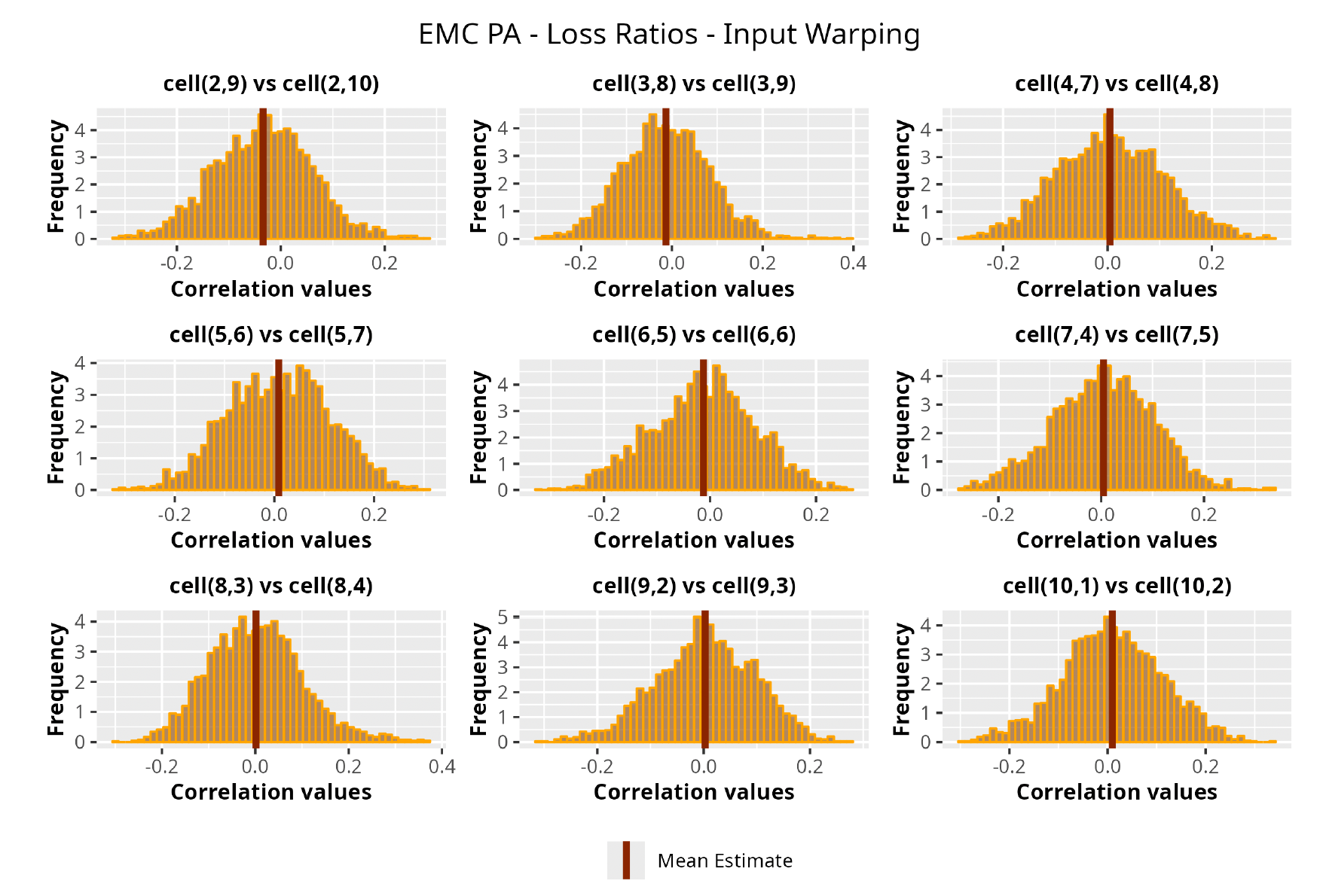
In Figures 13 to 17 we show the correlation between the leading diagonal, i.e., the current calendar year, and the subsequent one, i.e., the next calendar year, for each triangle and for each method. It is important to highlight that we are not analyzing the actual correlation values but their Fisher z-transformations; when the sample correlation coefficient is near the upper or lower boundaries, its distribution is highly skewed. The Fisher z-transformation solves this problem by yielding a variable whose distribution is approximately normally distributed (Wicklin 2017).

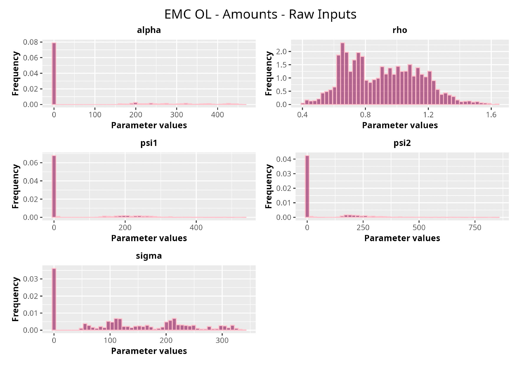
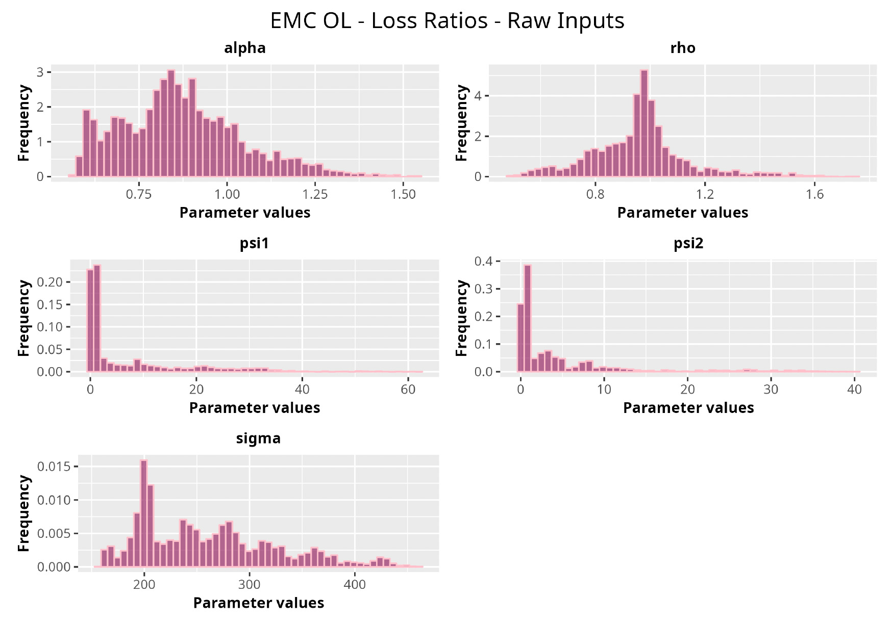
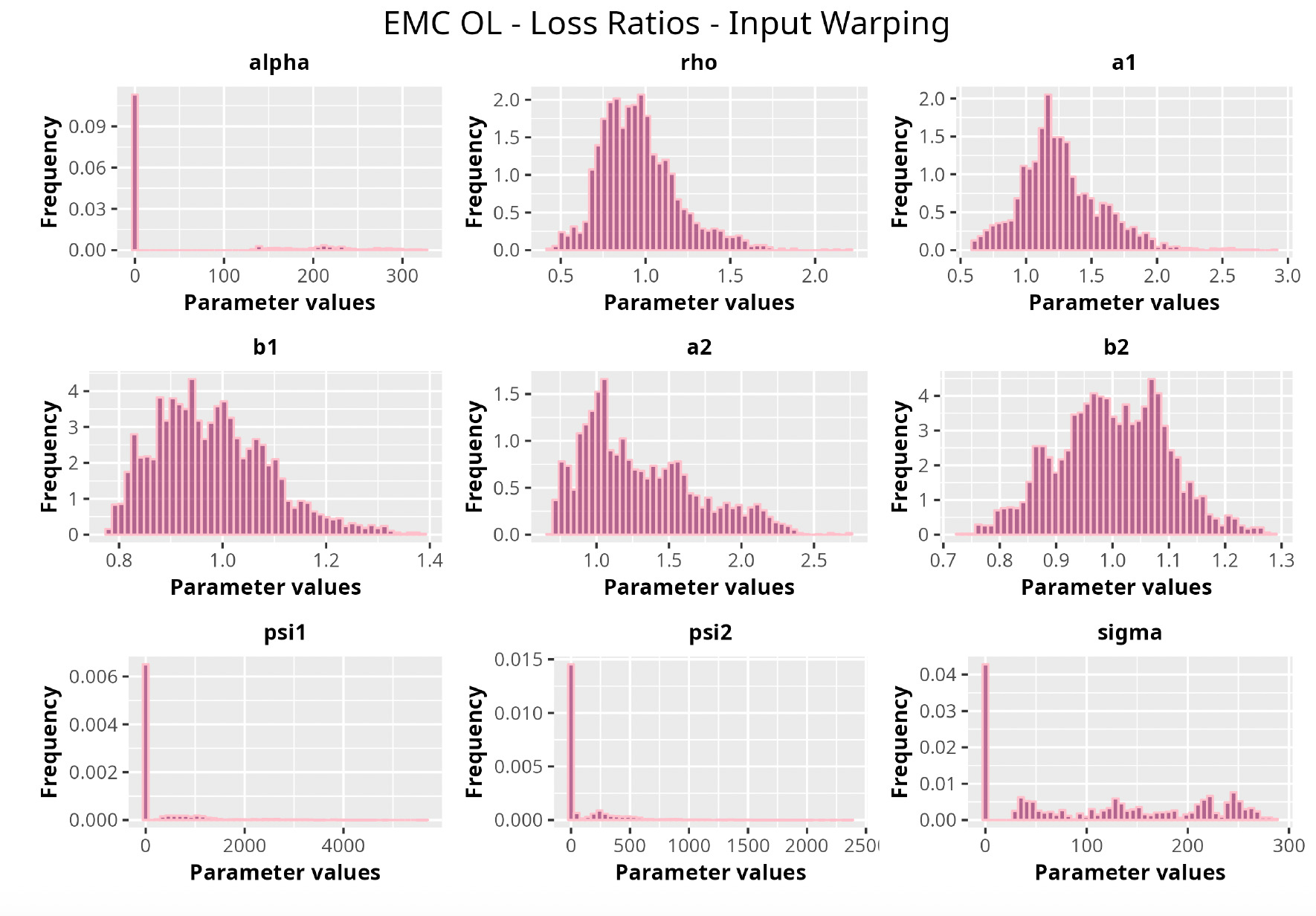
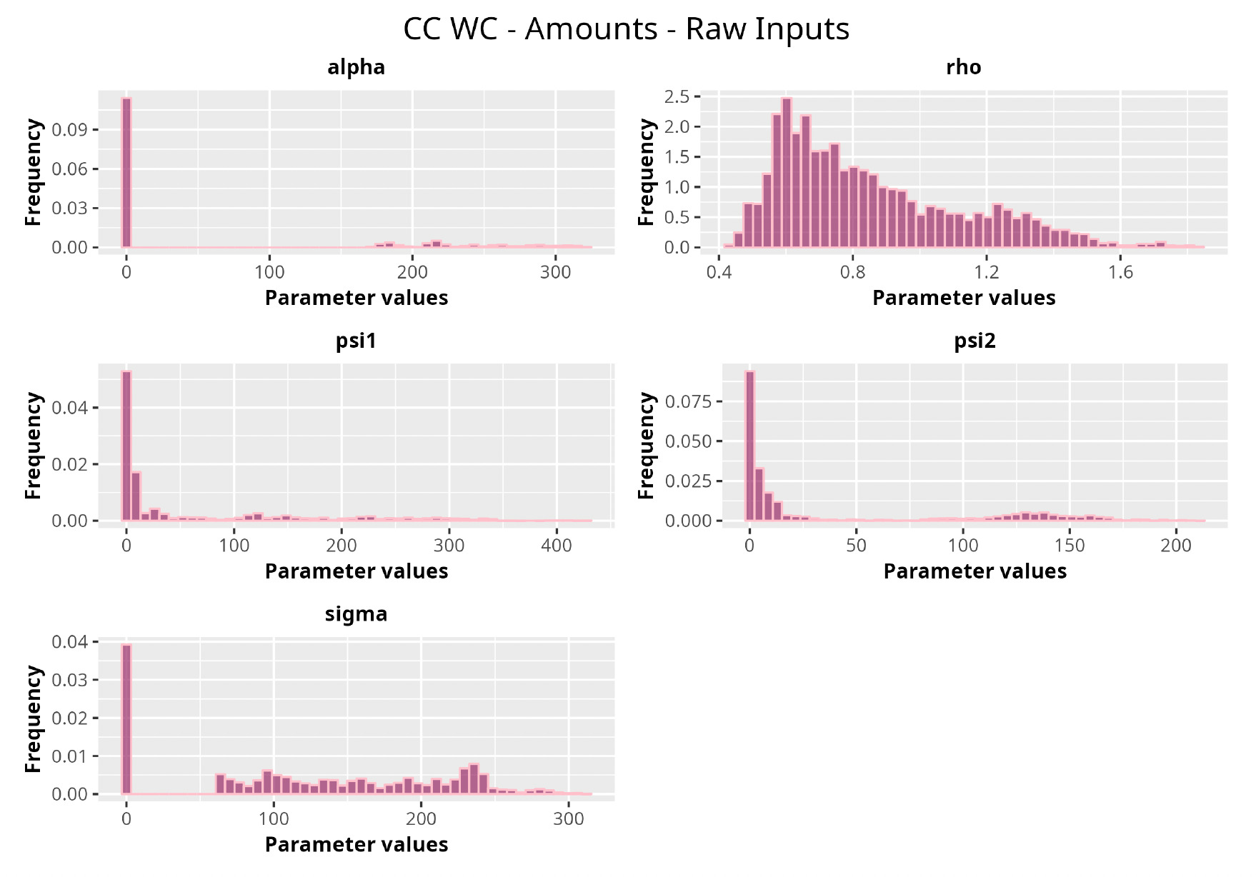
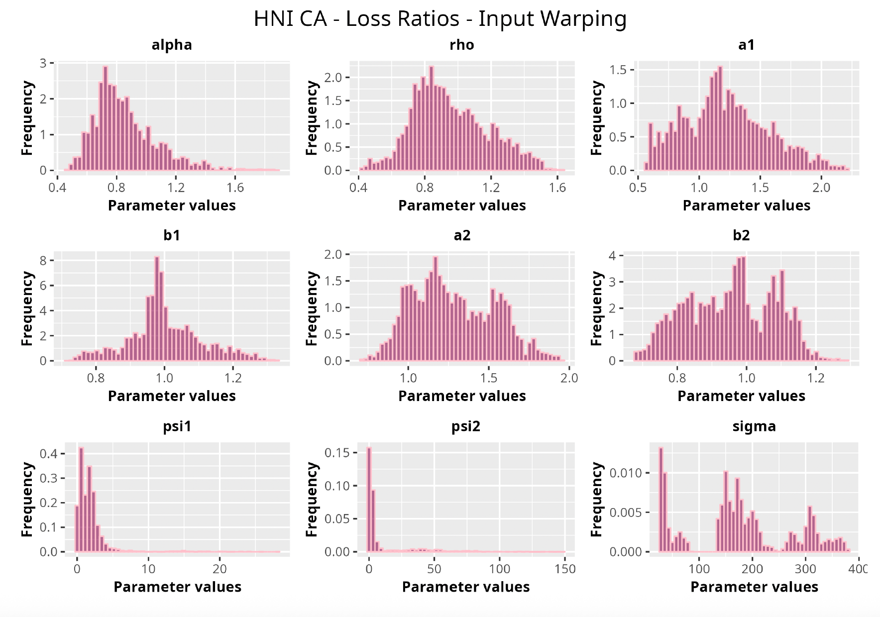
For completeness, in the appendix we also show the posterior distributions for all the individual pairs.

We can observe from the plots that, as expected given the specifics of the model, the average correlation is zero or near zero. This result implies that the amounts of payments during a calendar year, on average, do not affect the payments during the following year. The entire distribution, however, conveys more insight and information that can be used in several scenarios. From a risk management or capital requirement perspective, it is valuable to compute confidence intervals or specific percentiles on the distribution (e.g., VaR or TVaR) in order to estimate payments even in more remote eventualities that deviate from average values and can potentially cause financial impairment.

7.2. Loss development analysis

Next, we take a look at the loss development patterns and compare the expected versus observed cash flows. Such an exercise is useful for a variety of reasons and applications. One that we will explore is the possibility of applying loss development factors (LDFs) from one triangle (e.g., industry data) to another (e.g., company-specific data), a common practice when using Schedule T data to create a distribution of losses by state or in estimating due taxes under IRS reporting procedures (Odomirok 2020).

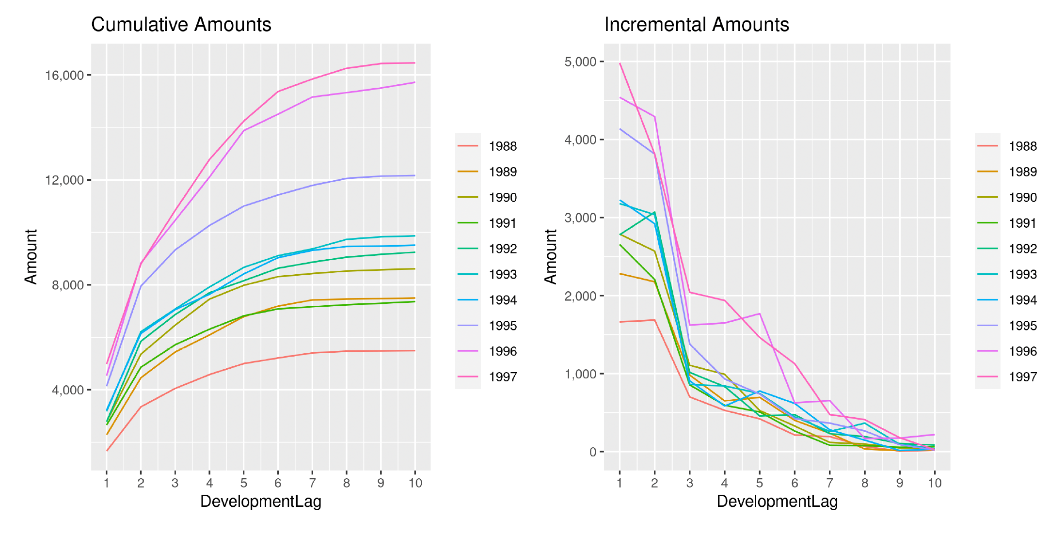
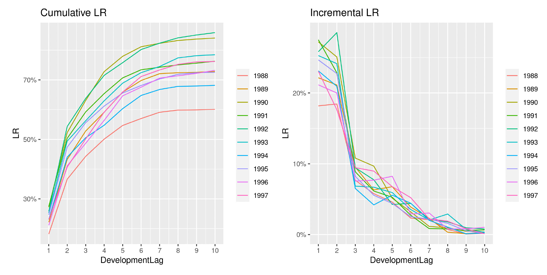
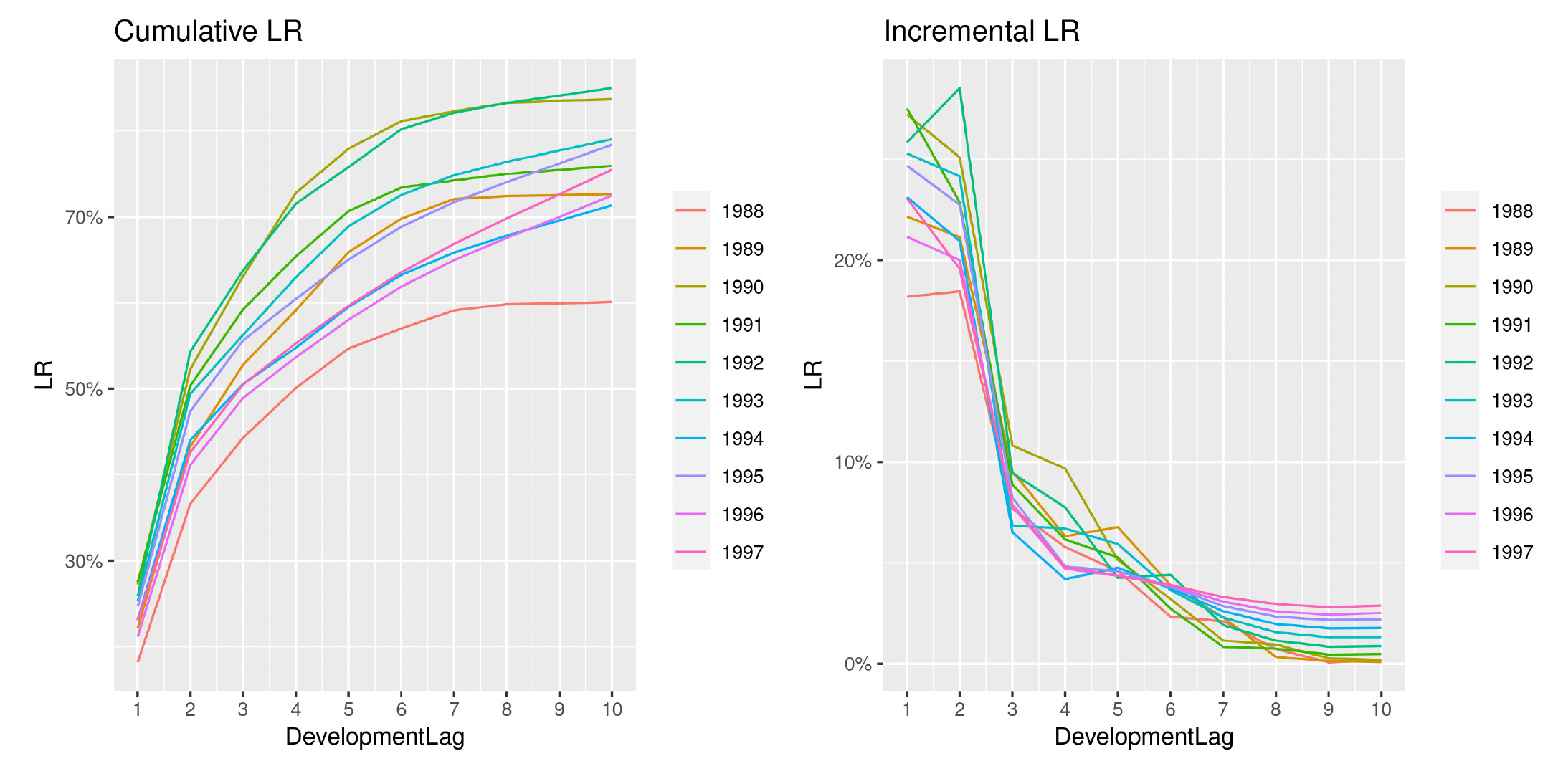
Directing our attention to one of the triangles analyzed (EMC PA) in the previous section, we show in Figures 18 and 19 the development of losses for both incremental and cumulative amounts, comparing the observed and the estimated ones.

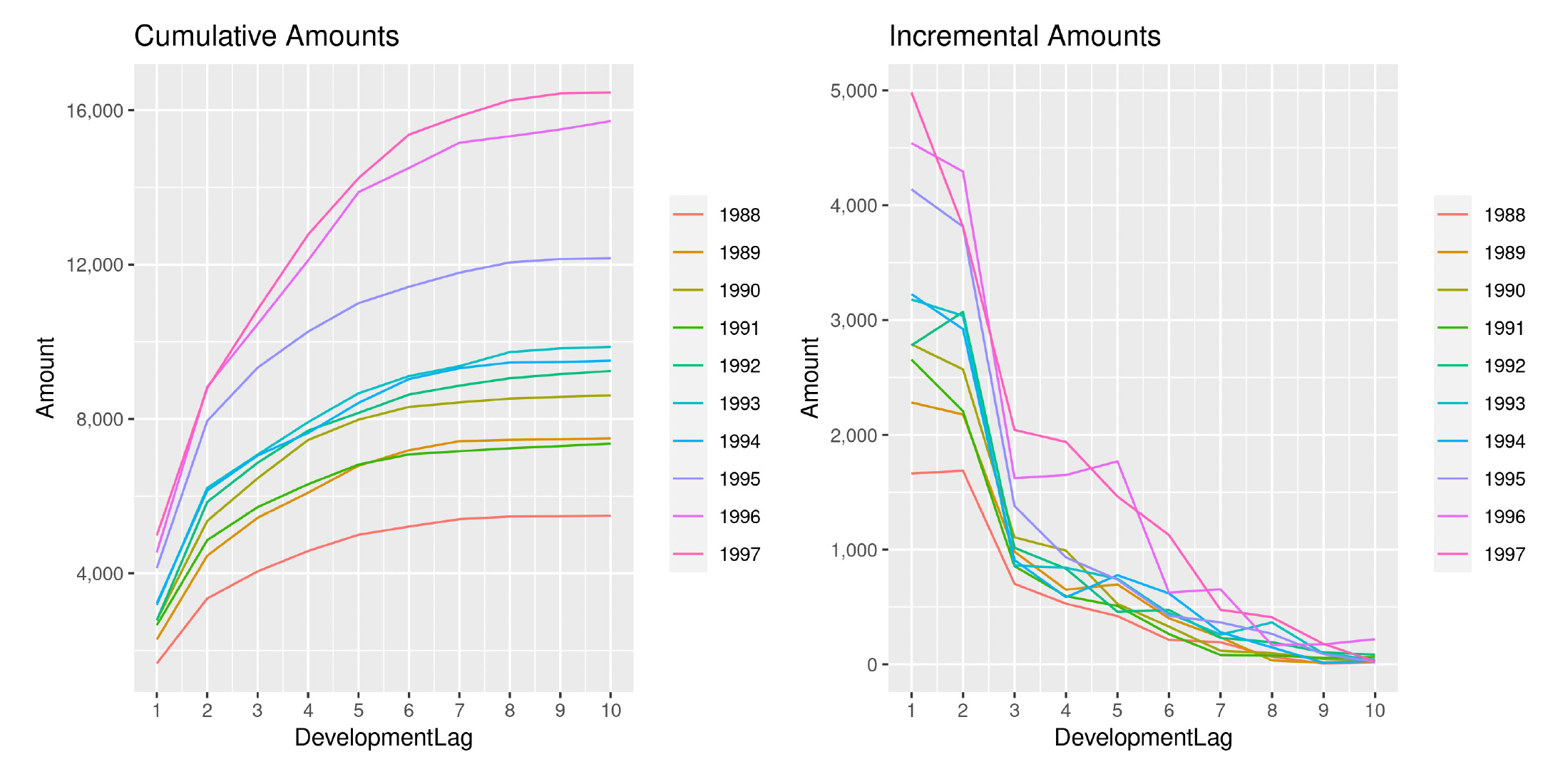
The two sets of graphs show the observed development of claim amounts and LRs until the ultimate value for each accident period. Thus we can appreciate how claims develop and the variability that affects the occurrence pattern. We can also understand why a more wiggly covariance function is able to better capture the payment pattern.

This is precisely the objective of choosing a specific function from among the ones available. It is important to understand the data and ensure that the chosen function is appropriate. Given the complexity of the methodology, an unsuitable choice could lead to inaccurate results.

Another interesting aspect is how the analysis of the LRs reduces the variability between AYs and has the effect of an implicit standardization of the claim amounts. We can, in fact, observe how the year-over-year claim inflation observable in Figure 18 is significantly reduced when compared to Figure 19. Moreover, the incremental patterns also appear more stable and less erratic.

It does not come as a surprise that GPR methodologies based on LR analysis are capable of producing more accurate results, in terms of both point estimates and stochastic robustness.

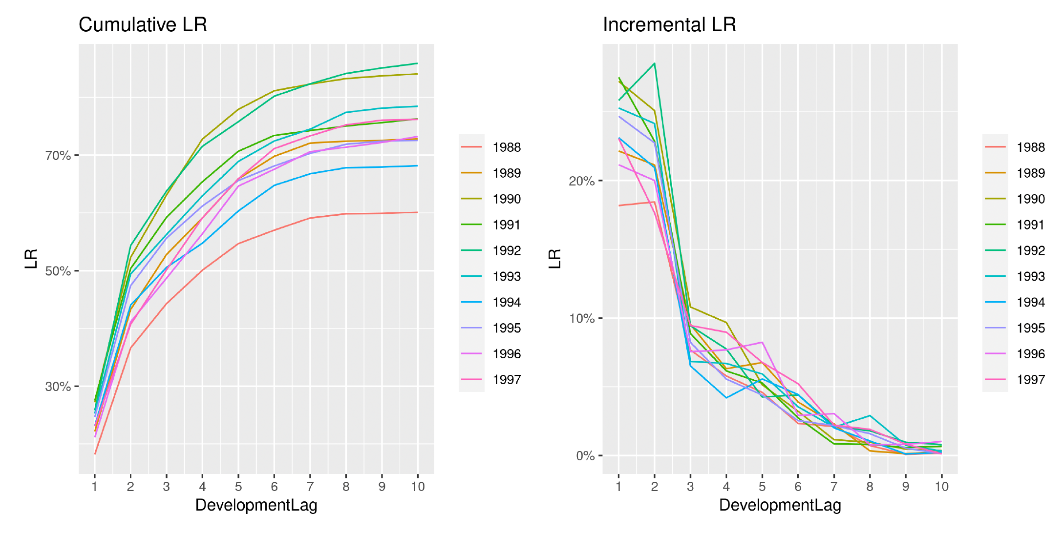
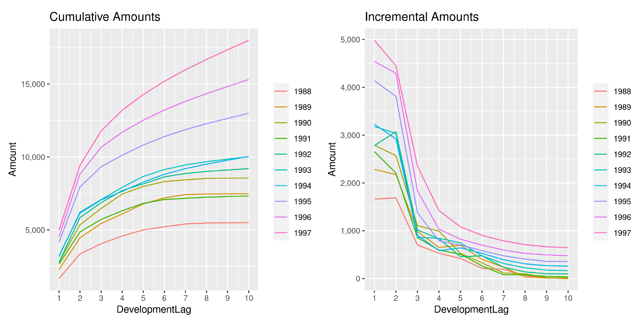
For completeness we shall compare observed patterns to estimated ones. In Figure 20, continuing the analysis from the previous section, we show the computed patterns based on observed claim amounts and LRs.

We can observe how the year-over-year effect is exacerbated and cumulative projections for very recent AYs appear to be too inflated and too regular, becoming less and less meaningful when compared to older AYs. This is due to the abundance of regularity introduced by the model in the estimation of incremental payments. As previously specified, the model is fit on incremental amounts rather than cumulative amounts.

We can observe this effect in the incremental patterns in Figure 20—the estimates for the most recent AYs are essentially older estimates just shifted upward.

This effect is removed when looking at LRs, shown in Figure 21, and the overall performances seem to improve.

These projections appear to be in line with the observed patterns, and they carry a very high level of accuracy. Including premiums in the analysis proves to be a good choice that has the potential to significantly increase the accuracy of the calculations. Overall, the GPR with the convolution between the Matérn 7/2 and the squared exponential covariance functions applied to the observed LRs led to the most accurate predictions. This behavior is due to two main reasons:

1. A more flexible covariance function better captures the real-world variability of data.

2. By using LRs, we can implement an initial standardization of the claims, which gives us more information about the insurance business, e.g., increased claim costs due to increasing business volumes rather than adverse experience.

7.3. Loss development uncertainty

In this last section, focusing on loss development patterns, we examine the role of estimated loss development patterns and the possibility of transferring and applying patterns between different sets of claims. This falls into the stream of actuarial work dedicated to loss development pattern analysis (Clark 2003; De Virgilis 2020), and it helps bridge the gap between traditional and more sophisticated methods. Because the GPR methodology is inherently stochastic, it is possible to extract LDFs from the distribution of future claims. It is also possible to create confidence intervals around them in order to produce optimistic and pessimistic scenarios.

This procedure can be useful when analyzing small sets of data, e.g., a newly established insurance business, which do not allow us to apply deterministic or stochastic methods in a robust and reliable way. Estimating LDFs on industry data and then applying the patterns on our data can still give us the possibility to develop the claims to their ultimate values and also to construct confidence intervals around them, a common procedure when producing the actuarial opinion summary (Committee on Property and Liability Financial Reporting 2018).

Figure 22 shows such patterns and their 95% confidence interval built with the GPR methodology.

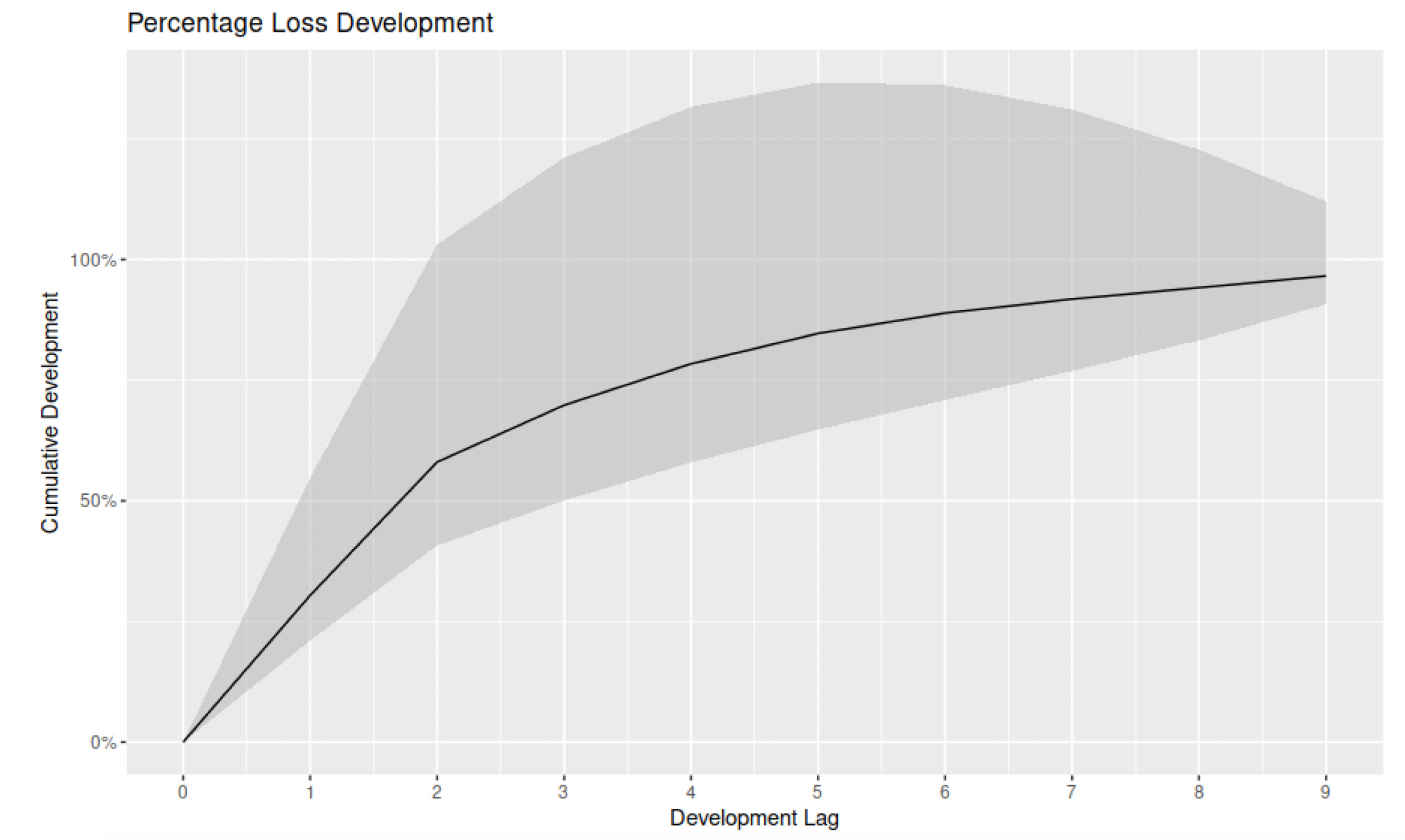
The graph shows the average LDFs alongside the 95% confidence interval. Such curves can then be applied to different sets of claims and also used to test patterns developed with other methods. The GPR methodology can, therefore, be used to enhance the accuracy of other estimates, providing an additional validation tool.

8. Conclusions

Overall, our intent in this paper is to provide the actuarial practitioner an overview of GPR techniques from both a theoretical and a practical standpoint. An example of a reproducible application is also provided. In so doing, we hope to spark interest in applying more advanced techniques that traditionally are not part of the classical actuarial toolkit. GPRs, in fact, have mainly been adopted in the context of geospatial statistics.

More precisely, the paper presents how to apply GPR techniques with several covariance functions in the context of actuarial loss reserving.

We implement an inverse Wishart distribution and several covariance functions alongside their combinations to fit multivariate Gaussian distributions, taking as input the AY and the DP through the use of beta input warping functions. We apply such models on incremental claim amounts as well as incremental LRs; the results are analyzed and compared against traditional methodologies found in the actuarial literature.

Our findings show that GPR models can outperform traditional techniques from a deterministic, as well as a stochastic, point of view. And given the nature of the method, we can also further investigate the distributions of the model parameters in order to further study the variability of the claim estimates. In a context where the stochastic behavior of the reserve estimate is valuable, such an approach can act as a hedge against more simplistic methodologies, e.g., ODP.

The methodology, as presented, could certainly be improved and refined. Further studies could focus on the implementation of different covariance functions such as the periodic covariance function or different orders of the Matérn formulation. Another area of improvement could be the introduction of further dimensions. In our study we employed the AY and the DP as inputs. However, in some contexts where inflation is an important factor to consider (e.g., structured settlements analysis), using the calendar year as an additional predictor could bring additional value.

Overall, this work shows the additional value that the implementation of GPRs could bring to the actuarial sciences. There are, however, some inconveniences to consider before implementing a Bayesian framework. One of the main difficulties is the choice of prior distributions (Lemoine 2019). Another complication that may arise is related to the technological infrastructure; complex inference analysis may require long runtimes.

All of the analysis and the code used throughout the paper is public and available at the following GitHub repository: https://github.com/marcopark90/GaussianProcesses.

A preliminary summary of the paper results was presented at the CAS Annual Meeting on November 9, 2022:
https://www.casact.org/sites/default/files/2022-11/CS-5_Applications_of_Gaussian_Process_Regression_Models.pdf.

---

Acknowledgments

This work was sponsored by the Casualty Actuarial Society, the Actuarial Foundation’s research committee, and the Society of Actuaries’ Committee on Knowledge Extension Research. The authors wish to give special thanks to all the CAS staff who supported the ongoing research and to the anonymous reviewers who provided extremely useful insights that significantly improved the quality of our paper.

Finally, the opinions expressed in this paper are solely those of the authors. Their employers neither guarantee the accuracy nor the reliability of the content provided herein nor take a position on it.