Improved Estimation of Parametric Tail Factor Models

1. Introduction

A common challenge in actuarial practice is estimating how losses will develop beyond the point to which historical data is available. For example, an $N$-by-$N$ loss triangle may be available for a certain portfolio of business, but 2% of claims in the first accident year may still be open after a development lag of $N$ years. It would be unreasonable to assume that there will be no more loss payments on those open claims, and it would be equally unreasonable to assume that every open claim will eventually require payments up to policy limits. It is less unreasonable, but still unsatisfying, to assume that future loss payments will be exactly equal to case reserves at that point in time.

Standard loss development techniques can be used to estimate loss development from lag 1 year to lag 2 years, from lag 2 years to lag 3 years, and so forth. However, these techniques are typically unable to provide development factor estimates past the highest development lag available in the training data. The problem of extrapolating loss development patterns beyond the edge of a loss triangle is known as tail modeling and is typically framed in terms of estimating a tail factor that, when multiplied by the estimated losses as of lag $N$ years, yields the estimated ultimate losses.

Tail factor methods are typically important in two cases: when claims take a very long time to be reported and resolved, and when little historical data on loss development is available. In this paper, we concentrate more on the latter case. Estimating future claim payments associated with asbestos, sexual assault, and other causes of loss with exceptionally long reporting lags are typically better handled with techniques that explicitly incorporate domain-relevant knowledge, rather than relying on context-free curve-fitting.

1.1. Parametric extrapolation methods

Our focus in this paper is on the estimation of parametric extrapolation tail factor methods. We consider a parametric extrapolation tail factor method to be any method that satisfies the following criteria:

1. Given the estimate of losses for accident year $w$ at development lag $d$ (written $c(w, d)$), then the estimate of losses at the next development lag has the form $c(w, d+1) = c(w, d) \cdot f(d)$. We refer to the proportional factor $f(d)$ as the age-to-age (ATA) factor.

2. The estimated ATA factor at development lag $d$ years, $f(d)$, is a function that only depends on $d$.

3. $f(d)$ has a finite number of parameters $\{\beta_0, \beta_1, \dots\}$ that control its behavior.

4. The values of $\{\beta_0, \beta_1, \dots\}$ are estimated, directly or indirectly, from a loss triangle.

5. The tail development factor from development lag $n$ to infinity, $T(n)$, is defined as $\prod_{i=n}^\infty f(i)$.

A number of models in the literature conform to this basic structure. Six prominent examples are shown in Table 1, along with their functional forms and restrictions on the values of their parameters. References to further discussion of each of the models are provided. In some cases, the symbols used for the parameters in each of the models have been changed for the sake of uniformity.

The notation $F_W(d; \beta_0, \beta_1)$ indicates the cumulative distribution function of the Weibull distribution with parameters $\beta_0$ and $beta_1$ evaluated at point $d$.

The condition on the value of $\beta_1$ in the inverse power model is required to ensure that the tail factor from the inverse power curve is finite; see Evans (2014) for a rigorous proof of this.

In this paper, we focus on experiments with the exponential decay and inverse power models, which perform reasonably well in real-world circumstances. The inverse power model tends to yield larger tail factors than the exponential decay model, and unsurprisingly it tends to outperform other models on famously long-tailed lines of business such as workers’ compensation. The generalized Bondy model tends in practice to yield estimates that are nearly identical to those of the exponential decay model, the inverse power model tends to better predict tail estimates than the Weibull model, and the shifted inverse power and shifted Weibull models tend to be overparameterized, particularly given the sparse nature of tail development data.

1.2. Current estimation methods

In current practice, most parametric extrapolation tail methods are estimated by first selecting a set of ATA factors $\hat{f}(d)$ based on the available loss development triangle, then finding the values of the parameters $(\beta_0, \beta_1)$ that minimize some measure of error. The most common choice of error metric is the sum of squared log-incremental errors (SSLIEs):

$$SSLIE = \sum_{d=1}^D \left( \ln (f(d) - 1) - \ln (\hat{f}(d) - 1) \right) ^ 2. \tag{1}$$

In practice, there are a small handful of other common variations on this basic idea, such as minimizing the sum of squared errors between selected and fitted ATA factors, instead of between selected and fitted log-incremental ATA factors.

There are several reasons why ATA-based tail estimation methods are so popular. By operating on ATA factors rather than on triangles, the computational resources required to estimate a tail factor are significantly reduced. ATA factor selection is a standard part of almost any actuarial analysis that would also require a tail factor estimate, so the additional effort required to prepare ATA factors for the sake of inputs to the tail factor model is essentially zero. ATA factors are (essentially by construction) less volatile than the loss triangles on which they are based, so the estimation method can afford to be less robust to the presence of outliers. Finally, actuaries frequently exercise their professional judgment by manually adjusting one or more aberrant ATA factors, further smoothing the inputs to the tail factor model.

However, there are also some significant drawbacks to estimating tail models in this fashion. We will describe these drawbacks in more detail as we present our proposed alternatives.

2. Proposed estimation technique

2.1. Basic form

As an alternative to ATA-based methods, we propose to fit parametric development curves directly to the triangle itself. We can directly maximize

$$\small{ \begin{align}LLT &=\sum_{w=1}^W \sum_{d=1}^D \ln \phi \left( c(w, d+1) \; | \; f(d) \cdot c(w, d) \; , \; \sigma^2_{w,d} \right) ; \\w + d &\leq n + 1 \end{align} \tag{2} }$$

where $\phi(x | \mu, \sigma )$ represents the probability density of a gamma distribution with mean $\mu$ and variance $\sigma$ evaluated at a point $x$. (We are using the nonstandard notation $\phi(\cdot)$ here instead of $f(\cdot)$ because of the notational conflict with ATA factors.)

Here, the target label LLT stands for log-likelihood of triangle, because that is exactly what the optimization target is: the log-likelihood of the entire observed triangle, conditional on the development factor curve $f(d)$.

In theory, we could select any continuous distribution with at least two parameters and support over the positive reals for our choice of $\phi$. In practice, we have seen good results with this estimator by using the gamma distribution, which is efficient to evaluate and is a common choice of distribution in actuarial applications of generalized linear models. It is also easy to convert a given mean and standard deviation to corresponding parameters of a gamma distribution via the method of moments: the shape parameter $\alpha = \mu^2 / \sigma^2$ and the rate parameter $\beta = \mu / \sigma^2$.

Estimating the parameters of a parametric tail factor model directly from a triangle, rather than from ATA factors, has a couple of distinct advantages. First, the amount of data underlying each ATA factor is far from uniform. In particular, later ATA factors are based on a small handful of observed link ratios, even on the extreme of a single link ratio for the last ATA factor. This implies that later ATA factors are more volatile and that the sampling distribution of ATA factors is strongly dependent on development lag. By estimating the tail factor model parameters directly from the triangle, we sidestep these issues.

Second, the estimator Equation (1) is unusable if any of the ATA factors are less than 1.0. It is tempting to argue that an ATA factor below 1.0 is a sure sign that continued material tail development is no longer a concern, but unfortunately the truth is not so simple. Negative incremental development factors are not uncommon for smaller triangles, even on long-tailed lines of business with a significant amount of remaining development. By contrast, modeling cumulative losses as a gamma distribution means that our estimator works well as long as losses are strictly positive—a condition that is much easier to satisfy.

2.2. Functional form of variance

In the likelihood Equation (2), the variance component of the distribution is written as $\sigma^2_{w,d}$. The subscripts suggest that the modeled variance varies by cell, but it was not practical for us to estimate a separate value of $\sigma^2$ for every single cell in the triangle.

Instead of trying to use a large number of degrees of freedom to estimate the triangle’s variance as a function of development lag (as in Mack’s method), or assuming that variance is constant across the entire triangle, we choose to estimate variance with a relatively economical function of three variables:

$$\mathrm{Var}(c(w,d+1) | c(w,d)) = \exp(\psi_0 + \psi_1 \ln c(w,d) + \psi_2 d).$$

In effect, we are assuming that the two most important features that determine the variance of a cumulative loss amount are the volume of losses and the current development lag. Both of these features are easily justifiable on theoretical grounds, and some practical experimentation has revealed that including additional predictors of cumulative loss variance does little or nothing to improve goodness of fit. Intuitively, we expect that $\psi_1 > 0$ and $\psi_2 < 0$, and indeed this is what we see in practice.

The SSLIE estimator’s use of squared error as an optimization target means that the estimator is equivalent to assuming that log-incremental ATA factors are normally distributed with a constant variance. Due to the nature of the log-incremental transform, this implies that the variance of ATA factors decreases as the magnitude of the factors decreases. This basic tendency is similar to the effect of the $\psi_2$ parameter in our proposed estimator, but there is no a priori reason to expect that log-incremental ATAs should have exactly constant variance. In contrast, our parameterization allows the evidence to dictate exactly how much variance of link ratios decreases as a function of development lag.

2.3. Relevance weighting

If we fit our model by considering each of the observation pairs $(c(w, d), c(w, d+1))$ independently, it is natural to consider whether all of the observation pairs are equally relevant to the task of estimating the tail factor. We can construct a weighting function $\omega()$ that gives more or less weight to each observation based on its perceived relevance to the task at hand. (Traditionally, weighting functions are written as $w()$, but we already use the letter $w$ to index experience periods in loss triangles.)

There are two strategic objectives for which observation-level weighting is well suited: relevance weighting and recency weighting.

All of the tail factor models we consider in this paper assume that expected ATA factors follow some parametric function that depends on $d$. These parametric forms are generally chosen because they are reasonably effective at approximating the shape of empirical ATA factors for later development lags. However, these same parametric forms commonly do a very poor job of matching empirical ATA curves for early development lags. This is not terribly surprising. Loss development is a complex process, and assumptions about development that may be approximately true under steady-state conditions with almost all claims reported may not hold earlier in the development process, when claims behavior is more dynamic.

This observation suggests that, rather than fit tail curves to all of the available data in a loss triangle, we focus the tail-fitting effort on later development lags where the tail curve is a better approximation to the data. We refer to this idea as relevance weighting.

The crudest way to do relevance weighting is simply to drop all data prior to some minimum development lag $d^*$. This is simple and easy to implement, but the sharp cutoff for relevance isn’t necessarily realistic.

A better alternative is to use the cumulative log-log function:

$$\omega(w, d) = \exp\left( -\phi_1 \cdot \exp(\phi_0 - d) \right).$$

In this parameterization, the parameter $\phi_0$ represents the development lag at which there is an inflection point between less and more relevance weighting—effectively, the fuzzy analog to the minimum development lag $d^*$. The parameter $\phi_1$ represents sharpness of the transition from low to high relevance weights. As $\phi_1$ approaches infinity, the weighting function approaches a step function from 0 to 1 with the step at $d = \phi_0$. For lower values of $\phi_1$, the transition is more gradual.

The cumulative log-log function is asymmetric and in a way that lines up well with our intuition about relevance. It seems typical that there is some point on the x axis before which the behavior of the ATA factor curve is clearly dissimilar to the parametric assumptions of a tail factor method, but the point at which the ATA factor curve has clearly settled down is less obvious. The cumulative log-log function drops to zero very quickly for $d < \phi_0$, but the increase to 1 when $d > \phi_1$ is considerably more gradual. This nicely mirrors our intuition.

2.4. Recency weighting

The other type of observation-level weighting we find useful is recency weighting. Recency weighting simply puts more emphasis on more recent information. In the context of weighting loss triangles, it is typically most useful to apply recency weighting as a function of the accounting period $k = w + d$. Our goal in designing a recency weighting function is to give full weight to development information on the most recent available diagonal and progressively less weight to information from older accounting periods. A convenient functional form for recency weighting is

$$\omega(w,d)_{\textrm{Recency}} = \gamma ^ {(n - w - d + 1)}; 0 < \gamma \leq 1 ,$$

where $n$ is the total number of accident/development periods in the triangle. The exponential decay functional form assigns full weight to the most recent accounting period and allows weights to decrease smoothly for older accounting periods.

Besides its convenience and simplicity, there are reasonably strong theoretical grounds for preferring this functional form for recency weighting. If we assume that ATA factors for a given development lag $d$ follow a random walk process with respect to $w$, the optimal estimator for $\hat{f}(d)$ is an exponentially weighted moving average of the observed $f(d)$ values. By using exponential decay recency weighting, we are heuristically doing something similar to assuming that development lags follow a random walk. Of course, just as with the assumption that ATA factors are static, the assumption that ATA factors follow a random walk process is almost never exactly true—but this assumption is usually less wrong than assuming that ATA factors are perfectly static with respect to time.

2.5. Bayesian estimation

In our proposed tail factor estimation method, we have five separate parameters to estimate: $\phi_0$, $\phi_1$, and $\phi_2$ from the variance model, plus the $\beta_0$ and $\beta_1$ parameters that describe the development curve itself. This is a relatively large number of parameters to fit to a relatively small amount of data. Even when fitting a standard two-parameter tail factor model to a dozen or so data points, there are still times when it is reasonable and prudent for an actuary to step in and apply their professional judgment in order to manually adjust a parameter whose maximum likelihood estimate borders on the absurd.

In the context of a study to assess the empirical accuracy of tail factor estimation methods, it is impractical to employ actuarial judgment on thousands of triangles and judgmentally select parameter values for each one. Even if doing so were practical, it would raise questions as to whether any improvement in predictive accuracy should be attributed to the new estimation method or to the quality of actuarial judgment.

A convenient solution to this problem is to avoid estimating the tail model parameters for each triangle in isolation. Bayesian hierarchical estimation provides an attractive way to avoid the volatile estimates that maximum likelihood estimates fit to each individual triangle would produce, while still allowing parameters for each individual triangle to vary to the extent warranted by the data.

When we estimate tail factor models for a few dozen separate loss triangles, we do so by fitting all of the triangles simultaneously with a single Bayesian model, where values of $\phi_0$, $\phi_1$, and $\phi_2$ (the variance model parameters) are shared by all triangles, but $\beta_0$ and $\beta_1$ (the curve-specific parameters) are estimated hierarchically (or as random effects, in classical parlance). We applied reasonable, mildly informative priors to each of the parameters—just enough to discourage the model from exploring entirely improbable portions of the parameter space.

3. Data and comparison methodology

Given that our motivation is to develop an estimation method that is more accurate than extant techniques, it is imperative to compare the predictive accuracy of our method with the conventional baseline on a relatively large corpus of loss triangles—large enough that we can say with a reasonable degree of certainty that differences in accuracy are due to characteristics of the estimation methods themselves and not merely due to random chance.

It is easy enough to obtain a fairly large corpus of loss triangles from statutory filings. Schedule P of the annual statement contains 10-by-10 annual triangles for roughly a dozen lines of business. From that universe of data, we have curated a corpus of 8,193 10-by-10 loss triangles from Schedule P of annual statements, spanning accident years 1987 through 2021. The corpus covers four lines of business: medical liability (claims made basis), other liability (claims made basis), other liability (occurrence basis), and workers’ compensation. These four lines of business are all reasonably long-tailed, as measured by the ratio of paid to booked losses at development lag 10 years.

The corpus was curated by only considering annual statements from top-level NAIC entities and removing triangles with less than $10 million of mean net earned premium per accident year for that line of business. We further removed triangles where less than 50% of gross premium in that line of business was retained on a net basis, because Schedule P triangles are presented on a net basis, and complex reinsurance structures could potentially distort development patterns. Finally, we removed a handful of clear outlier triangles in the data.

Summary statistics of the corpus are presented in Table 2.

3.1. Measuring tail model performance

One of the essential challenges of tail modeling is that the task is one of extrapolation rather than interpolation. If we are trying to estimate a tail factor $T_n$, it is almost always because we have no data past development lag $n$. In spite of the obvious data limitations, there are two methods we can use to estimate the performance of tail factor methods on statutory data: we refer to these as censoring and proxying. Both of these methods are obviously inferior to comparing model predictions to true ultimate losses $c_\mathrm{paid}(w, \infty)$, but they represent complementary strategies for making the best use of the limited available data. If both methods indicate that one estimation technique is superior to another, this serves as strong evidence of a material difference in the predictive performance of the techniques.

3.2. Censoring

In censoring, we artificially limit the amount of data available to estimate the tail factor. We can fit a tail factor to data $c_\mathrm{paid}(w, d)$ where $w + d \leq n'$ for some $n' < n$. For example, on statutory data, where $n = 10$, we could fit a tail model to an $n' = 7$ year triangle. Given the parametric curve fit to this limited data, we can then construct an estimate of $\hat{c}_\mathrm{paid}(1, 10)$ as $c_\mathrm{paid}(1, 7) \cdot f(7) \cdot f(8) \cdot f(9)$. Given that all of the parametric development curves we are considering provide explicit estimates for every $f(d)$, this is entirely feasible. Given our restricted estimate of $\hat{c}_\mathrm{paid}(1, 10)$, we can compare this against the true hold-out value $c_\mathrm{paid}(1, 10)$.

Censoring suffers from the problem that we are only measuring the extrapolation performance of the tail factor curve over a relatively short time horizon of a few years. It could be that an estimation method works well for fitting development curves in the near future but degrades significantly when extrapolating into the distant future. This happens fairly often in practice, typically when a very low degree of decay in ATA factors yields good predictions for the next handful of development lags but gives implausibly large tail factors when carried many years further.

3.3. Proxying

In proxying, we rely on the fact that Schedule P data includes several measures of losses: paid losses, which we denote as $c_\mathrm{paid}(w, d)$; reported losses (i.e., paid loss plus case reserves but excluding incurred but not reported (IBNR) reserves and bulk reserve adjustments, often referred to in the literature as “incurred” losses), which we denote as $c_\mathrm{rptd}(w, d)$; and booked losses (i.e., reported losses plus IBNR reserves and bulk reserve adjustments), which we denote as $c_\mathrm{book}(w, d)$.

The proxy measurement of tail performance compares a tail factor–based estimate of ultimate loss $\hat{T}_n \cdot c_\mathrm{paid}(1, n)$ against $c_\mathrm{book}(1, n)$. This does not require any unavailable data and is out-of-sample with respect to the model because the model was only trained on paid losses.

Proxying is problematic because it assumes that actuarial estimates of ultimate losses (i.e., the booked losses) are accurate and unbiased estimates of what the true ultimate losses will be. There are many historical examples of booked losses, even at 10 years’ development, being materially wrong. Companies routinely revise their estimates of older accident years, which is reflected in the “Prior Years” row in Schedule P, Sections 2–4.

However, these problems do not mean that proxying is a meaningless measure or that proxying is just an exercise in pitting one tail factor estimate against some other tail factor fit by another actuary to the same data. In general, actuaries on staff at an insurance company have significantly more information available than what is revealed in Schedule P, such as triangles that extend beyond 10 years, claims files for potentially large losses that are still pending, and detailed breakdowns of losses at a finer degree of granularity than statutory lines of business.

3.4. Implementation of the SSLIE estimator

Given that we are studying tail model predictive performance on a large corpus of backtest data, we do not have the luxury of hand-selecting ATA factors for every triangle. Even if it were logistically feasible, it would not necessarily be desirable, as the performance of the estimation method would be intrinsically linked to the quality of the ATA factors fed into the method and therefore to the skill of the person exercising actuarial judgment in selecting the ATA factors. To sidestep this, we will consider all ATA factors to be traditional chain-ladder volume-weighted averages, without any regularization or smoothing:

$$\hat{f}(d) = \frac{\sum_{w=1}^{n-d-1}c(w+1,d)}{\sum_{w=1}^{n-d-1}c(w,d)}.$$

As noted earlier, the SSLIE estimator cannot easily handle $\hat{f}(d)$ values that are less than or equal to 1.0. Our simple adjustment for handling these cases is to replace all $\hat{f}(d)$ below $f_{crit} = 1.001$ with $f_{crit}$. The choice of 1.001 for $f_{crit}$ appears to be a reasonable trade-off between eliminating extreme outliers and avoiding adjustments to too many ATA factors.

3.5. Implementation of the proposed Bayesian estimator

When using our Bayesian hierarchical estimator, we partitioned the triangles in the backtest corpus by line of business and maximum accident year. For example, all 10-by-10 workers’ compensation triangles with latest accident year 2002 were fit via the same Bayesian hierarchical model.

Rather than performing full stochastic sampling from the posterior distribution for each model, we simply took the maximum a posteriori parameter values. We used Stan’s implementation of L-BFGS as the optimizer (Carpenter, Gelman, Hoffman, et al. 2017).

Within a Bayesian context, it is difficult to directly estimate values of the weighting parameters $\gamma$, $\phi_0$, and $\phi_1$. Optimization of the weighting parameters would be best performed by a difficult and time-consuming hyperparameter optimization exercise. In lieu of that, we use the values $\gamma = 0.85$, $\phi_0 = 4$, and $\phi_1 = 1$ as reasonable values that should be adequate to show at least some benefit over flat weighting.

4. Results

For this study, we measure model performance as the root mean square of the log-scale predictive error. For censoring, the error term is defined as

$$\epsilon = \ln \hat{c}_\mathrm{paid}(1, 10) - \ln c_\mathrm{paid}(1, 10),$$

and for proxying, the error term is defined as

$$\epsilon = \ln \hat{c}_\mathrm{paid}(1, 10) - \ln c_\mathrm{book}(1, 10).$$

Our proposed method for estimating tail factors deviates from commonplace methodology in at least seven respects:

1. Fitting the development curve to a loss triangle rather than a set of selected ATA factors.

2. Assuming that cumulative losses are gamma-distributed rather than implicitly assuming that (cumulative or incremental) ATA factors are normally or log-normally distributed.

3. Directly estimating the variance of one-step-ahead development errors from the data itself rather than assuming constant variance.

4. Giving less weight to older observations within the triangle rather than weighting all observations equally.

5. Letting weight as a function of development lag vary via a complementary log-log function rather than imposing a hard cutoff.

6. Using informative Bayesian priors on tail model parameters rather than estimating via maximum likelihood.

7. Estimating tail factors for multiple triangles simultaneously via a hierarchical model structure rather than estimating each triangle’s tail factor independently.

It is natural to question the extent to which each of these individual differences contributes to any overall difference in predictive performance of the tail factor method as a whole. If, for example, it turns out that the vast majority of the improvement comes from item (4) above, then it would be much easier to implement that change by itself into a standard actuarial workflow, as opposed to using an entirely new and relatively complex tail factor estimation methodology.

However, the sheer number of differences in methodology makes attribution fairly challenging. If each of the differences is considered as an independent binary choice, there are 128 possible estimation methods to evaluate. If we consider the fact that some of these differences contain additional degrees of freedom (for example, the coefficients in the complementary log-log weighting function, the parameterization of the variance function, and the priors on the model parameters), we are faced with evaluating thousands of alternatives.

As a compromise, we compare our proposed tail factor estimation methodology with two alternatives. The first alternative is plain SSLIE estimation, without any of the methodological changes we are proposing. The second is a Bayesian hierarchical version of SSLIE with relevance weighting—effectively, the combination of differences (5), (6), and (7) above.

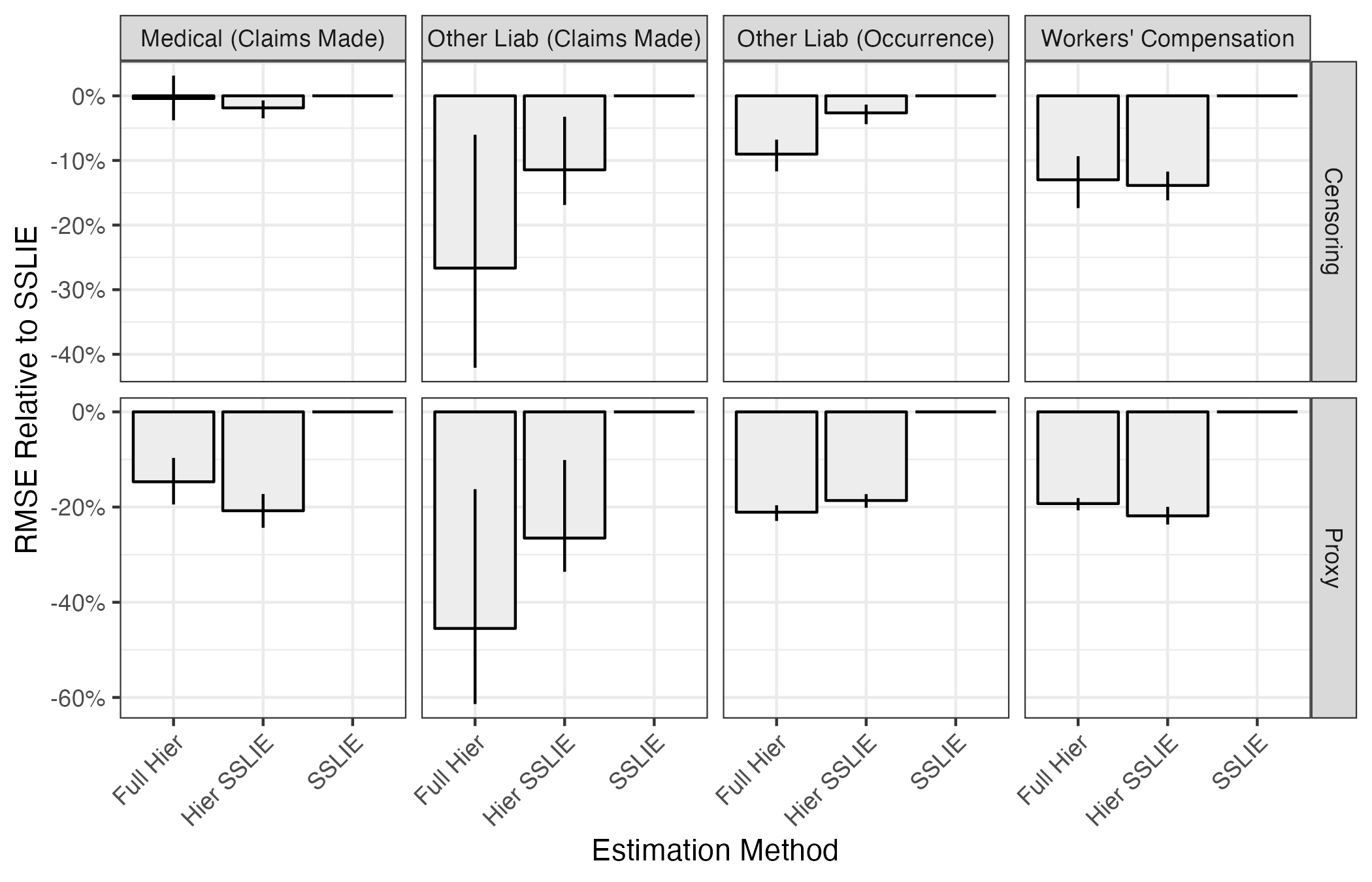
In Figure 1, we show the performance of our proposed method (labeled as Full Hier), the hierarchical version of SSLIE (labeled as Hier SSLIE), and the traditional implementation of SSLIE for the exponential decay tail model. Each subplot shows predictive accuracy for a specific line of business and predictive basis of comparison (i.e., censoring or proxy). Within each subplot, the height of each bar represents the relative ratio of a given estimator’s root mean square error (RMSE) against the RMSE of the SSLIE estimator, which we take as a baseline. For example, within the Other Liability (Claims Made) Censoring subplot, we see that the hierarchical version of the SSLIE estimator yields an RMSE reduction of almost 15% against baseline SSLIE, and the full hierarchical estimator yields an RMSE reduction of about 25%. The vertical lines on each bar represent a 90% bootstrap confidence interval (CI) of the relative RMSE between that estimator and the SSLIE estimator. A 90% bootstrap CI that includes 0% is a sign that the difference between those two estimators may be due to random noise.

Figure 1.Comparison of predictive performance of three alternative estimators for the exponential tail factor model.

We present the same information in tabular form in Table 3. In the table, we present the actual RMSE values rather than relativities to the SSLIE estimator. The final two columns show a 90% bootstrap CI of the absolute difference between that estimator and the SSLIE estimator, which is why those values are always missing from the SSLIE estimator.

In nearly all cases, using a hierarchical estimator instead of simple SSLIE improves tail factor estimation—sometimes to a dramatic extent. RMSE for hierarchical estimators is consistently about 20% lower on a proxying basis than the SSLIE estimator, which equates to a reduction in predictive variance of about 40%. The difference between the two hierarchical variants is less dramatic, but our proposed estimation method appears to have a persistent and material performance advantage for the two other liability lines of business.

In Figure 2 we show corresponding results for the inverse power tail factor model. Other than the change of model, the structure of the plot is the same. Similarly, Table 4 shows these results in tabular form.

Figure 2.Comparison of predictive performance of three alternative estimators for the inverse power tail factor model.

The approximate direction of effects here is much the same as for the exponential model, but the magnitude of the effects is significantly greater. Both of the other liability lines of business had their RMSEs cut more than 50% by switching from the traditional SSLIE estimator to our proposed estimation method. The intuition behind this result is that the inverse power tail model tends to generate heavier tail factors than the exponential method, and maximum likelihood estimates of inverse power curves can lead to extremely large tail factor estimates. The regularization benefit from the hierarchical estimation approach is greater for the inverse power model because its tail factor estimates are less stable.

5. Conclusion

The methodology for estimating tail factors proposed in this paper consists of several separate suggested enhancements. These recommendations, taken as an entire suite, offer clear improvement in predictive performance, as evidenced by our backtest study. However, significant improvements in tail factor estimation can still be achieved simply by fitting tail models in a hierarchical context, without making the switch to triangle-based estimators.