Adjusting Manual Rates to Own Experience: Comparing the Credibility Approach to Machine Learning

1. Introduction

Using market data to aid in setting own company rates has been a common practice in the insurance industry. External data, as provided by insurance rating bureaus (e.g., Appendix A.1), reinsurers, or advisory organizations, supplement internal company data that may be scarce or unreliable because it is not representative, has a short history, or does not yet exist (e.g., when a new business line or a new territory is entered). According to Porter and American Institute for Chartered Property Casualty Underwriters (2008), pools of insurers in the US existed as early as the second part of the 19th century. These pools supported their members in setting rates through data collection and standardized policy forms. In the first part of the 20th century, the McCarran Fergusson Act partially exempted the insurance industry from the US federal antitrust regulation; thus National Association of Insurance Commissioners (NAIC) laws explicitly allowed cooperation in setting rates and specified the role of rating organizations. The importance of external data has been historically recognized by regulators to support adequate rates that preserve a company’s solvency, prevent excessive competition, and ease the entrance of new players (e.g., granting a partial antitrust law exemption in the US jurisdiction; Danzon 1983).

When the insurer takes its own experience into account to enhance the credibility of its rates, it must benchmark its portfolio experience compared with that of the market. The actuarial profession traditionally used techniques based on Bayesian statistics and nonparametric credibility to optimally integrate market and insurer portfolio experiences into the technical rates. From this viewpoint, the market data contribution satisfies the two classic approaches addressed by credibility theory: the limited fluctuation credibility theory and the greatest accuracy credibility theory (e.g., Norberg 2004). The former refers to incorporating individual experience into the rate calculation to stabilize the level of individual rates. The latter corresponds to applying modern credibility theory and combines both individual and collective experiences to predict individual rates by minimizing mean square error.

Credibility theory is extensively used in non-life insurance. Early models were not based on policyholders’ ratemaking variables (see, e.g., Bühlmann and Gisler (2006) for a comprehensive presentation). The actuarial literature has proposed some advanced regression credibility models, such as the Hachemeister model (Hachemeister and others 1975). Conversely, rates based on generalized linear models (GLMs), the current gold standard in personal rate pricing (Goldburd, Khare, and Tevet 2016), are based solely on the impact of ratemaking factors, giving no credit to the individual policy experience.

Nevertheless, mixed effects GLMs allow incorporating policyholders’ experience within the GLM tariff structure (Xacur and Garrido 2018; Antonio and Beirlant 2007); however, they are not widely used. All these regression approaches enable insurers to incorporate individual risk profile covariates into a credibility model. The structure of insurance data, notably the distinction between own experience and market experience, is dealt with in the hierarchical credibility model of Bühlmann and Straub (1970). In some situations, the use of company data is not possible at all and only a tariff at market level is reliable.

For instance, in France, a two-level Bühlmann-Straub rating model is used for fire and business interruption insurance (Douvillé 2004), with data collected from the French association of private and mutual insurers. In other countries, to the best of the authors’ knowledge, public insurance bureaus exist in Italy, Germany, the UK, and Brazil. The Italian Association of Insurers aggregates data from the motor lines (but only pure premiums with few covariates) and long-term care insurance for health, while it collects extensive statistics (with many covariates) for crop insurance. The German Insurance Association provides data similar to that of the Italian association for many lines. The industry data and subscription section of the Association of British Insurers provides (at least) yearly aggregate data for many property and casualty, health, and life line of business categories. Finally, the Brazilian Insurance Regulator (SUSEP) provides aggregated losses and exposures for motor liability insurance aggregated by key rating variables.

Credibility theory is also largely used in life insurance applications for modeling mortality risks. A first attempt to stabilize mortality rates by combining the mortality data of a small population with the average mortality of the neighboring populations was proposed by Ahcan et al. (2014). Regarding this issue of limited mortality data (small population or short historical observation period), Li and Lu (2018) introduced a Bayesian nonparametric model for benchmarking a small population compared with a reference population. Bozikas and Pitselis (2019) focused on a credible regression framework to efficiently forecast populations with a short base period. To improve mortality forecasting, some recent contributions in the literature combine the usual mortality models, such as the Lee and Carter (1992) model and the Bühlmann credibility theory (Bühlmann and Gisler 2006; see also, Tsai and Lin 2017; Tsai and Zhang 2019, and Tsai and Wu 2020, among others).

The recent widespread use of machine learning (ML) has provided many more techniques for practitioner actuaries. Gradient boosting models (GBMs) and deep learning models (DLs) for motor third-party liability pricing are presented in Noll, Salzmann, and Wuthrich (2020), Ferrario, Noll, and Wuthrich (2020), Schelldorfer and Wuthrich (2019), and Ferrario and Hämmerli (2019). More recently, Hanafy and Ming (2021) showed that the random forest technique is more efficient for predicting claim occurrence (in terms of accuracy, kappa, and area under the curve values) than are logistic regression, XGBoost, decision trees, naive Bayes, and k-nearest neighbors algorithm. Matthews and Hartman (2022) compared random forest, GBM, and DL against GLM to predict claim amount and claim frequency for commercial auto insurance and demonstrated its efficiency and accuracy for future ratemaking models. Henckaerts et al. (2021) also showed that GBMs outperform classical GLMs and allow insurers to form profitable portfolios and guard against potential adverse risk selection. Furthermore, researchers have applied non-pricing approaches. For example, Spedicato, Dutang, and Petrini (2018) modeled policyholder behavior; Rentzmann and Wuthrich (2019) presented recent advances in unsupervised learning for vehicle classification as DL autoencoders; Kuo (2019) used the NAIC reserving dataset to show how neural networks with embedding may offer better prediction on tabular loss development triangles. Blier-Wong, Cossette, et al. (2021) conducted a comprehensive review of ML in property and casualty studies. On the life insurance side, applying DL to lapse modeling (Kuo, Crompton, and Logan 2019) and the DL version (Richman and Wuthrich 2019) of the classical Lee-Carter model are worth mentioning. For a more comprehensive review, see Richman (2021b, 2021a). Recently, Diao and Weng (2019) combined credibility and regression tree models. In these presentations, the ultimate goal of using ML was to improve the usual regression setup in actuarial science based on the GLM. However, techniques such as GBM and DL can also be used to transfer what the model learned on a much bigger dataset (e.g., market data) to a smaller dataset (e.g., company portfolio data). Transfer learning reuses knowledge learned from different data sources to improve learner performance. This ML area has become particularly popular in recent years, especially in computer vision DL modes to fine-tune standard architectures on specific recognition tasks (see Zhuang et al. (2021) for a comprehensive review). In our experience, such approaches tend to develop in the insurance industry for ratemaking models with the incorporation of new data sources (Blier-Wong, Baillargeon, et al. 2021), but they can also be used in other areas, for instance, to train life insurance valuation models (Cheng et al. 2019).

Our study aim was to take advantage of ML to more easily handle complex nonlinear relationships, as compared with standard credibility-based approaches, to more accurately assess policyholder risk. Hence, our work contrasts traditional methods with those of ML for blending market data into individual portfolio experience. First, we anticipated a difference between the credibility approach and the ML used in this study. The credibility approach naturally uses a longitudinal structure to calibrate its parameters, but this is not a prerequisite for ML models, which only need to share some variables. We applied our approach on a (properly anonymized) dataset comprising both market and own portfolio experience from a European non-life insurance pool. Final comparisons focused not only on predictive performance, but also on practical applicability in terms of computational demand, ease of understanding, and interpretability of results.

The rest of this paper is organized as follows. We review the hierarchical Bühlmann-Straub (HBS) credibility model in Section 2. Section 3 presents the main ML algorithms used in this paper. Section4 compares the performance between ML and HBS models based on a market dataset and a company dataset, and Section 5 concludes this paper.

2. Hierarchical credibility model

This section briefly describes the hierarchical credibility theory of Bühlmann and Gisler (2006), which we used to model claim frequency. We also refer to Goulet (1998) for a general introduction.

Consider a large portfolio of $I$ individual risks, which includes heterogeneous risk profiles as well as market and company data. The model is defined as an unbalanced claim model since different claim histories are available across individual risks. Intrinsically, the credibility approach is based on a longitudinal data structure where individual/policyholder clusters are repeatedly observed for a given period. Generally, the company data experience is shorter than that of the market. In addition, we assumed that market and company datasets share the same features, which allows them to fit into a framework compatible with homogeneous transfer learning approaches (Zhuang et al. 2021).

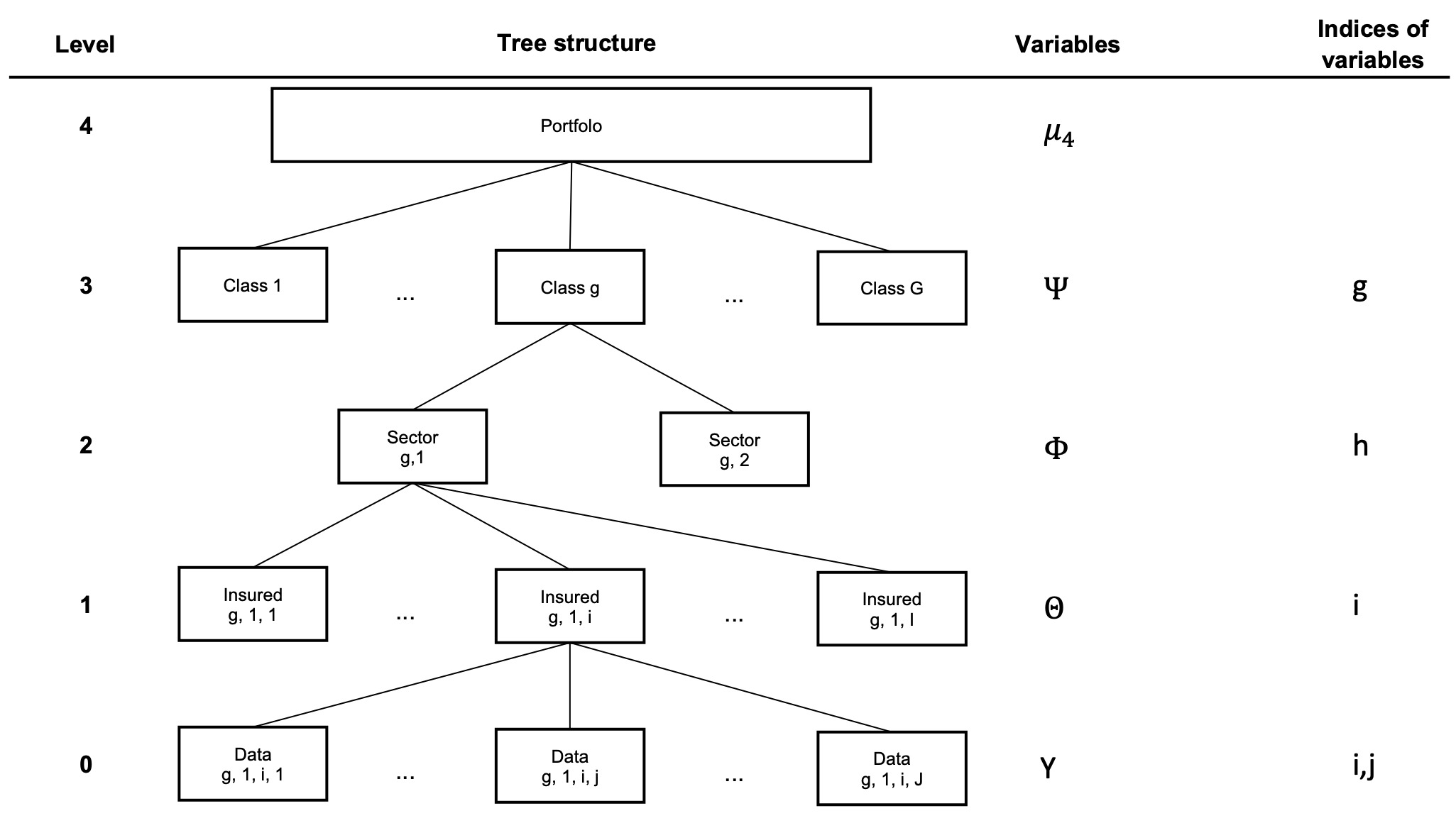
For the ease of this presentation and without a loss of generality, we used a five-level model structured in a hierarchical tree, as presented in Figure 1, with the usual notation. The five levels are presented from top to bottom, based on the classical assumptions of hierarchical credibility theory:

Figure 1.Representation of a five-level hierarchical tree structure.

• Level 4: This is the entire portfolio with market and company information.

• Level 3: The portfolio is divided into risk classes. We introduced parameters related to this risk level, $\Psi_g$, $g = 1,\ldots, G$, which are independent and identically distributed.

• Level 2: Each risk class is divided into sectors. Given $\Psi_g$, we denote by $\Phi_{g,h}$, $h=1,\dots, H$ the class risk parameters, which are assumed to be conditionally independent and identically distributed.

• Level 1: Given $\Phi_{g,h}$, $\Theta_{g,h,i}$, $i=1,\ldots,I$ are the individual risk parameters, which are conditionally independent and identically distributed.

• Level 0: Given $\Theta_{g,h,i}$, data are available during the study period $[1,J_{g,h,i}]$. We denote by $\mathbf{Y}_{g,h,i} = (Y_{g,h,i,1}, \ldots, Y_{g,h,i,J_{g,h,i}})$, the vector of observations over years, which are conditionally independent, identically distributed, and have a finite variance. We also introduce a vector for the relative known weights $\mathbf{w}_{g,h,i} = (w_{g,h,i,1}, \ldots, w_{g,h,i,J_{g,h,i}})$ over the same observation period.

In Section 4.2, the class variable related to Level 2 results from a combination of several categorical variables. These variables comprise unobservable risk factors that allow partitioning of the data space. Seven variables build up the credibility tree in the numerical application. That is, by adding intermediary levels in Figure 1; we consider 10-level hierarchical trees later in this paper.

To estimate credibility rates, we defined the following notations and structural parameters for $i=1, \ldots, I$ and $j=1, \ldots,J_{g,h,i}$:

• Level 4: Define $\mu_4=E[Y_{g,h,i,j}]$ the collective rates.

• Level 3: Define $\mu_3(\Psi_g)=E[Y_{g,h,i,j} \mid{\Psi_g}]$ for observations $Y_{g,h,i,j}$ that stem from $\Psi_g$, $\sigma_3^2(\Psi_g) = Var[\mu_2(\Phi_{g,h})\mid{\Psi_g}]$ and $\sigma_3^2 = Var[\mu_3(\Psi_g)]$.

• Level 2: Define $\mu_2(\Phi_{g,h})=E[Y_{g,h,i,j} \mid{\Phi_{g,h}}]$ for observations $Y_{g,h,i,j}$ that stem from $\Phi_{g,h}$, $\sigma_2^2(\Phi_{g,h}) = Var[\mu_1(\Theta_{g,h,i})\mid{\Phi_{g,h}}]$ and $\sigma_2^2 = E[\sigma_3^2(\Psi_{g})]$.

• Level 1: Define $\mu_1(\Theta_{g,h,i})=E[Y_{g,h,i,j} \mid{\Theta_{g,h,i}}]$ for observations $Y_{g,h,i,j}$ that stem from $\Theta_{g,h,i}$, $\sigma_1^2(\Theta_{g,h,i})) = Var[Y_{g,h,i,j} \mid{\Theta_{g,h,i}}] w_{g,h,i,j}$ and $\sigma_1^2= E[\sigma_2^2(\Phi_{g,h}))]$.

• Level 0: Define $\sigma_0^2= E[\sigma_1^2(\Theta_{g,h,i}))]$.

Similar to the Bühlmann-Straub model, the credibility estimates for these parameters are based on the Hilbert projection theorem (see Chapter 6 of Bühlmann and Gisler (2006)). With the above notations, we obtained the following classical results for hierarchical (inhomogenenous) credibility estimators $$\widehat{\mu(\Psi_g)}=\widehat{\alpha_g^{(3)}}\widehat{B_g^{(3)}} + (1-\widehat{\alpha_g^{(3)}})\widehat{\mu_4},$$ $$\widehat{\mu(\Phi_{g,h})}=\widehat{\alpha_{g,h}^{(2)}}\widehat{B_{g,h}^{(2)}} + (1-\widehat{\alpha_{g,h}^{(2)}})\widehat{\mu(\Psi_g)},$$ $$\widehat{\mu(\Theta_{g,h,i})}=\widehat{\alpha_{g,h,i}^{(1)}}\widehat{B_{g,h,i}^{(1)}} + (1-\widehat{\alpha_{g,h,i}^{(1)}})\widehat{\mu(\Phi_{g,h})},$$ where the credibility factor formulas $\widehat{\alpha_g^{(3)}}$, $\widehat{\alpha_{g,h}^{(2)}}$, $\widehat{\alpha_{g,h,i}}^{(1)}$ and weighted means $\widehat{B_g^{(3)}}$, $\widehat{B_{g,h}^{(2)}}$ and $\widehat{B_{g,h,i}^{(1)}}$ are given in Appendix A.6. The weighted means depend on structural parameters that can easily be estimated nonparametrically. Therefore, an HBS model provides a recursive computation of weighted empirical means whose parameters minimize quadratic losses. There are no distribution assumptions when deriving estimators; thus HBS models are full nonparametric models.

3. Modeling approach with transfer learning

This section presents the transfer learning (TRF) based framework, as well as ML models used in this paper. This research aimed to compare the predictive power of traditional credibility and ML methods that use an initial estimate of loss costs (from MKT experience) to predict those of a smaller portion (from CPN experience) in a subsequent period (the test set). Therefore, following the idea of the greatest accuracy credibility theory, our modeling process aimed to predict losses for the last available year (the test set) by training models on the experience of previous years, eventually split into training and validation sets.

3.1. Transfer learning

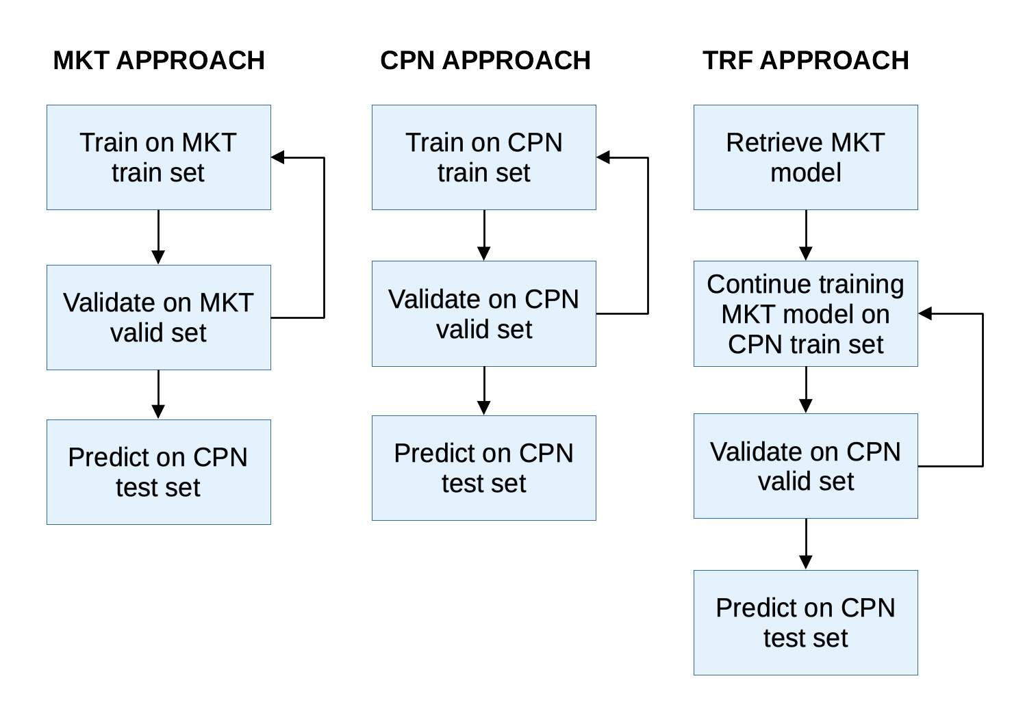
Figure 2 describes the main steps of our TRF approach compared with ML models fully trained on a market training dataset (MKT approach) or on a company dataset (CPN approach). To fit an ML model via the MKT approach (respectively, the CPN approach), we split the historical data from a benchmark (respectively, company) dataset solely between training and validation subsets. Then, performance was assessed based on test data from the company dataset.

The TRF approach relies on experience from the MKT approach and used the corresponding pretrained model as a starting point. Next, we fine-tuned the MKT model based on experience from the CPN dataset. The resulting model contained both information from the market and the company, and it should offer better predictions.

Figure 2.ML models training diagram.

3.2. Machine learning models

Next, we focused on ML models that permit an initial estimate of losses performed on another set via transfer learning. While we explored the use of such approaches applying ML methods, traditional GLMs may be used as well (see Appendix A.7 for a brief introduction). GLMs can perform log-linear regressions to estimate both the frequency and severity of the claim. These outputs can be used as offsets in subsequent models. For instance, under a log-linear regression framework and initial log estimate of the frequency, the severity of the pure premium may be set as an offset for a subsequent model (Yan et al. 2009).

ML methods used for insurance pricing are strongly nonlinear and can automatically find interactions among ratemaking factors while excluding nonrelevant features. In particular, two techniques are acquiring widespread importance, boosting and deep learning. Both techniques allow the use of an initial estimate of loss or exposure to risk to train the model on previous observations.

All ML models used in this work hold the Poisson assumption. That is, each i-th insurance policy is described by independent claim count $N_i$ such that $$N_i \sim \mathcal{P}oi\left(\lambda(x_i) \times v_i\right), i \in 1, \ldots, n,$$ where $x_i$ is the covariates’ vector and $v_i$ is the exposure related to the i-th policy for a sample of size $n$. Thus, ML models try to find the best functional form for $\lambda\left(.\right)$ by minimizing the Poisson loss function, typically on the test set $$L(\lambda(.))=\frac{1}{n}\sum_{i=1}^{n}{2n_i \left[\frac{\lambda\left(x_i\right)v_i}{n_i} -1-\textrm{ln}\left(\frac{\lambda\left(x_i\right)v_i}{n_i}\right)\right]},$$ where $n_i$ are observed claim counts.

3.2.1. Boosting techniques

The boosting approach (Friedman 2001) can be synthesized by the following formula $$F_t\left(x\right)=F_{t-1}\left(x\right)+\eta \times h_t\left(x\right).$$ That is, the prediction at the $t$-th step is given by the contribution, to the prediction of the previous step, of a weak predictor $h_t\left(x\right)$, properly weighted by a learning (shrinkage) factor $\eta$, where $x$ is the covariate vector. The most common choice for the weak predictor $h_t\left(x \right)$ lies in the classification and regression trees (CART) family (Breiman 2017), from which the gradient boosted tree (GBT) models take the name. CARTs partition the feature space in an optimal way to receive (more) homogeneity on the resulting subsets (in terms of the modeled outcome). Such optimal partitioning is determined by recursively searching for the stage-wise optimal split among all standardized binary splits (SBS). At first stage, given an optimal partition of size $K>0$ of the feature space, $(X_k^{(1)})$ with $k=1,2,…K$, the estimated frequency is constant in each element of the partition and determined by the maximum likelihood estimate

$$\hat{\lambda}_k = \frac{\sum\limits_{i=1}^{n}{\mathbf{1}_{\lbrace x_i \in X_k^{(1)}\rbrace}n_i} }{\sum\limits_{i=1}^{n}{\mathbf{1}_{\lbrace x_i \in X_k^{(1)}\rbrace}v_i}}.$$

As presented by Noll, Salzmann, and Wuthrich (2020), a weak learner is an SBS with just one split (e.g., $K=2$ leaves) such that the estimated frequency is

$$\lambda^{\left(1\right)}(x_i) = \hat{\lambda}_1\mathbf{1}_{\lbrace x_i \in X_1^{(1)}\rbrace}+\hat{\lambda}_2\mathbf{1}_{\lbrace x_i \in X_2^{(1)} \rbrace}.$$

The boosting approach starts from an initial estimate given by the above formula. We define working weights as $w_i =\hat{\lambda}^{\left(1\right)\left( x_i \right)}v_i$, so that $N_i$ follows a Poisson distribution, $\mathcal{P}oi\left(\mu(x_i) \times w_i\right)$. With a new SBS partition set $X^{(2)}$, we can recursively estimate $\mu(x_i)$ using a supplementary SBS such that

$$\hat \mu^{\left(2\right)}(x_i) = \left( \hat \mu_{1}^{\left(2\right)}\mathbf{1}_{\lbrace x_i \in X_1^{(2)}\rbrace}+\hat \mu_{2}^{\left(2\right)}\mathbf{1}_{\lbrace x_i \in X_2^{(2)} \rbrace} \right)^\eta,$$

where $\hat \mu_{1}$ and $\hat \mu_{2}$ are estimated using analog formulas as the first step. We obtain an improved regression function $\lambda^{\left(2\right)}(x)=\lambda^{\left(1\right)}(x) \times \hat \mu^{\left(2\right)}(x)$. The $\eta\in (0,1]$ parameter is the learning (shrinkage) factor and is used to make the learner even weaker, as values close to zero move the learner toward one. The estimation can be iterated $M$ times. Since it is performed in log scale, this reduces to the formula exposed at the beginning of the paragraph.

Boosting weak predictors leads to very strong predictive models (Elith, Leathwick, and Hastie 2008). Almost all winning solutions of data science competitions held by Kaggle are at least partially based on the eXtreme Gradient Boosting (XGBoost) algorithm (Chen and Guestrin 2016), the most famous GBT model. More recent and interesting alternatives to be tested are LightGBM (Ke et al. 2017), which is particularly renowned for its speed, and Catboost (Prokhorenkova et al. 2017), which introduced an efficient solution for handling categorical data.

The structural difference between XGBoost and LightGBM lies in the approach used to find tree splits. XGBoost uses a histogram based approach, where features are organized in discrete bins on which the candidate split values of the trees are determined. LightGBM focuses attention on instances characterized by large error gradients where growing a further tree would be more beneficial (leaf-wise tree growth). In addition, a dedicated treatment is given to categorical features. In general, none of these algorithms systematically outperforms the others on any given use case. Outcomes depend on the specific dataset and chosen hyperparameters (Gursky, n.d.; Nahon 2019). We chose LightGBM mainly because it is significantly faster than XGBoost, a definitive benefit when there is need to iterate the training through different combinations of hyperparameters. CatBoost was not considered because it is less mature compared with the other two algorithms.

A set of hyperparameters defines a boosted model, and even more defines a GBT model. The core hyperparameters that influence boosting are the number of models (trees), $t=1,2,\ldots, T$ (typically between 100 and 1,000) and the learning (shrinkage) rate $\eta$, with a typical value between 0.001 and 0.2 $h_t\left(x\right)$, and can be, when it belongs to the CART family, the maximum depth, the minimum number of observations in final leaves, or the fraction of observations (rows or columns) that are considered when growing each tree. The optimal combination of hyperparameters is learned using either a grid search approach or a more refined approach (e.g., Bayesian optimization).

When applied to claim frequency prediction, hyperparameters are fit to optimize a Poisson log loss function. In addition, to handle uneven risk exposure, the log measure of exposure risk is given (in log scale) as an init score ($F_t\left(x\right)$) to initialize the learning process. The init score (or base margin) in the boosting approach has the same role as the traditional GLM offset term (Goldburd, Khare, and Tevet 2016).

3.2.2. Deep learning

An artificial neuron is a mathematical structure that applies a (nonlinear) activation function to a linear combination of inputs, i.e.,

$$\phi\left( z \right) = \phi\left(< x_i , \bar w>+\beta\right),$$

where $\bar w$ and $\beta$ are the weights and the intercept, respectively. Popular choices of activation functions are the sigmoid $\phi\left( z \right) = 1/(1+\exp(-z))$, the hyperbolic tangent $\tanh\left( z \right)$, and the rectifier linear unit $\phi\left( z \right) = z \mathbf{1}_{\lbrace z \ge 0\rbrace}$. A neural network consists of one or more layers of interconnected neurons that receive a (possibly multivariate) input set and retrieve an output set (Goodfellow, Bengio, and Courville 2016). Modern deep neural networks are constructed of many (deep) layers of neurons. Deep learning has received increased interest for a decade, thanks to increased availability of massive datasets, increased computing power (in particular GPU computing), and newer approaches to reduce overfitting that prevented widespread adoption of such techniques in previous decades. Different architectures have reached state-of-the-art performance in many fields. For example, convolutional neural networks achieved top performance in computer vision (e.g., image classification and object detection; Meel 2021), while recurrent neural networks (see, e.g., Hochreiter and Schmidhuber (1997) for long short-term memory neural networks) provide excellent results for natural language processing tasks like sequence-to-sequence modeling (translation) and text classification (sentiment analysis). For applications in actuarial science, we refer to the recent review of Blier-Wong, Cossette, et al. (2021), and to the work of Richman (2021b, 2021a) for deep neural networks.

Simpler structures are needed for claim frequency regression. Multilayer perception architecture basically consists of stacked simple neuron layers, from the input layer to the single output layer. This structure handles the relationship between ratemaking factors and frequency (the structural part). Thus, holding the Poisson assumption, $N_i \sim \mathcal{P}oi\left(\lambda(x_i)\times v_i\right)$, the structural part is modeled as $\lambda(x_i) = \beta_0+\sum_{j=1}^{Q}{\beta_j\phi\left(z_i\right)}$, where $Q$ is the number of neurons of the preceding hidden layer. To handle different exposures, the proposed architecture is based on the solution presented by Ferrario, Noll, and Wuthrich (2020) and Schelldorfer and Wuthrich (2019). A separate branch collects the exposure $v_i$, applies a log transformation, and then this exposure is added in a specific layer just before the final layer (which has a dimension of one).

Training a DL model involves providing batches of data to the network, evaluating the loss performance, and updating the weights in the direction that minimizes training (back-propagation). The whole dataset is provided to the fitting algorithms many times (epochs) split into batches. A common practice to avoid overfitting is to use a validation set where the loss is scored at each epoch. When it starts to systematically diverge, the training process is stopped (early stopping).

4. Numerical illustrations

This section compares prediction performance between our ML and credibility models. We conducted the analysis on two real and anonymized datasets, CPN and MKT, preprocessed and split into training, validation, and test sets as discussed in Section 3.1. As mentioned previously, the predictive performance of the fitted models is assessed on the company test dataset, even if models have been calibrated on the company or the market datasets or both. Then, the models are fitted on the training set and predictive performance is assessed on the test set. The validation set is used in the DL and LightGBM models to avoid overfitting. Finally, the models are compared in terms of predictive accuracy, using the actual/predicted ratio, and risk classification performance, using the normalized Gini index (NGI) (Frees, Meyers, and Cummings 2014). The NGI has become quite popular in actuarial academia and among practitioners for comparing competing risk models.

Let $y_i$ be the actual number of claims ranked by their modeled score $v_i \times \hat \lambda\left(x_i\right)$. NGI is defined as $$NGI=\frac{2 \sum\limits_{i=1}^{n}{i y_i}}{n \sum\limits_{i=1}^{n}{y_i}}-\frac{n+1}{n}.$$ In addition to the NGI, we also compute the mean absolute error (MAE) and the root mean square error (RMSE), which are also popular metrics for comparing predictive performance (see Appendix A.2).

4.1. Dataset structure

Two anonymized datasets were provided, one for the market (mkt_anonymized_data.csv) and one for the company (cpn_anonymized_data.csv), henceforth referred to as MKT and CPN datasets, respectively (see Appendix A.4). These datasets share the same structure, as each company provides its data to the pool in the same format. The pool aggregates individual filings into a market-wide file that is provided back to the companies. It is important to note that the MKT dataset includes CPN data. The dataset contains the year-to-year exposures and claim numbers, aggregated by categorical variables. Losses are the number of damaged units, while exposures are the number of insured units. Therefore, only the frequency component has been modeled as the ratio between the claim number and the exposure. Henceforth, losses in this paper are considered a synonym for claim numbers. Our aggregated dataset contains the variables listed below:

• exposure: the insurance exposure measure, on which the rate is filled (aggregated outcomes)

• claims: the number of claims by classification group (aggregated outcomes)

• zone_id: territory (aggregating variable)

• year: filing year (aggregating variable)

• group: random partition of the dataset into training, validation, and test sets

• cat1: categorical variable 1 available in the original file (aggregating variable) (This can be considered a risk classification and, possibly, the most important predictor. The number of exposures insured strongly depends on this variable. Also, the cat1 distribution can vary significantly between companies.)

• cat2: categorical variable 2, available in the original file (aggregating variable)

• cat3: categorical variable 3, available in the original file (aggregating variable)

• cat4–cat8: categorical variables related to the territory (joined to the original file by zone_id)

• cont1–cont13: numeric variables related to the territory (joined to the original file by zone_id)

• entity: a categorical variable either CPN or MKT

Variable names, levels, and numeric variable distributions are masked and anonymized for privacy and confidentiality purposes. Categorical and continuous variables are anonymized by label encoding and scaling (calibrated on market data).

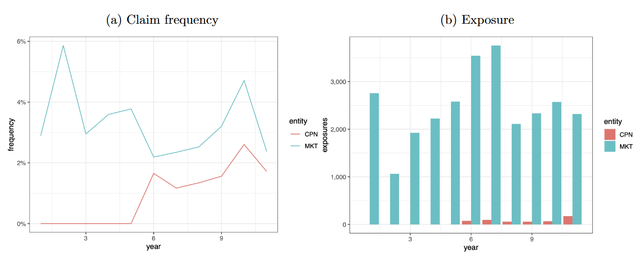
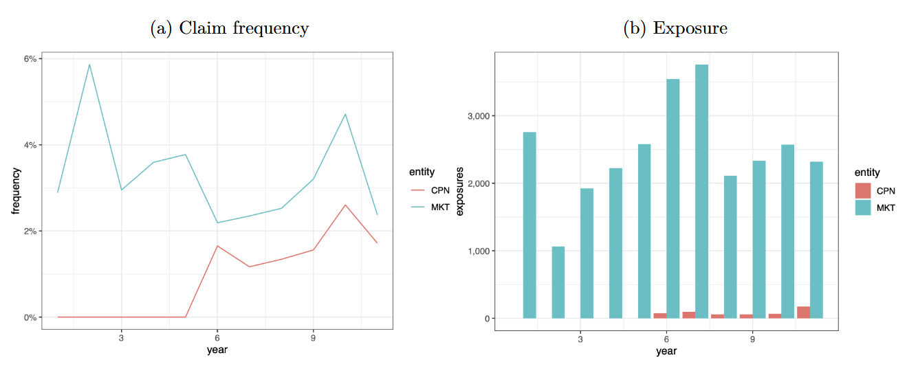
Figure 3 displays exposures and claim frequencies by year for each entity (MKT, CPN). Furthermore, the last available year (2008) is used as the test set, while data from previous years are randomly split between training and validation sets on an 80/20 basis (see Table 1). Market data are available for 11 years and company data for the last five years. Also, the number of exposures is widely dependent on the cat1 variable.

Figure 3.Claim frequences and exposures.

Tables 2 and 3 compare explanatory variables by domain. The frequency distribution is reported for categorical variables, while summary statistics are computed for continuous variables (mean, standard deviation, minimum, and maximum). The zone_id and cat1 statistics are shown in Appendix A.5 for the sake of synthesis. Note also that the variable year is not taken as an explanatory variable for the ML or credibility models. We implicitly assumed that the claims process was stationary.

4.2. Implementation details

This section presents the operations performed on the data and the implementation of the models. Dataset preprocessing was performed in a Python 3.8 environment, using the Pandas and Scikit-Learn libraries (Reback et al. 2020; Pedregosa et al. 2011) for the extraction, transformation, and loading stages. R Software (R Core Team 2022) and Python programming language were used for the analyses.

4.2.1. Boosting approach

The LightGBM (LGB) model was used to apply boosted trees on the provided datasets, minimizing the Poisson deviance. As for most modern ML methods, an LGB model is fully defined by a set of many hyperparameters for which default values may not be optimal for the given data. Indeed, there is no close formula to identify the best combination for the given data.

Therefore, we performed a hyperparameter optimization stage. For each hyperparameter, a range of variations is set, then a 100-run trial is performed using a Bayesian optimization (BO) approach performed by the hyperopt Python library (Bergstra, Yamins, and Cox 2013). Under the BO approach, each subsequent iteration is performed toward the point that minimizes the loss to be optimized, which is the loss distribution by hyperparameter updated for each iteration using a Bayesian approach. As suggested by boosting trees practitioners (Zhang and Yu 2005), the number of boosted models is not estimated under the BO approach but determined by early stopping. The loss is scored on the validation set and the number of trees chosen is the value beyond which the loss stops decreasing and starts diverging up.

The CPN and MKT models used the standard exposure (in logarithm base) as init score. The TRF model instead used as init score the a priori prediction of the MKT model on the CPN data. The LightGBM Python library was used for the boosted models (Ke et al. 2017). Computation was performed on an AMD-FX 9450 processor with 32 GB RAM. In general, fitting one model took about a minute on average in this environment.

4.2.2. Deep learning

Several approaches may be considered for building a DL architecture. Since the hyperparameter space of a DL architecture is vast, designing the best search strategy and network architecture (number of layers, number of neurons within, search, etc.) is challenging. Many practitioners start with a known working architecture for a similar task and perform moderate changes. It is also worth mentioning that more sophisticated approaches to DL architecture optimization are being developed (e.g., the neural architecture search; Elsken, Metzen, and Hutter 2019), but presenting such techniques is beyond the scope of this paper.

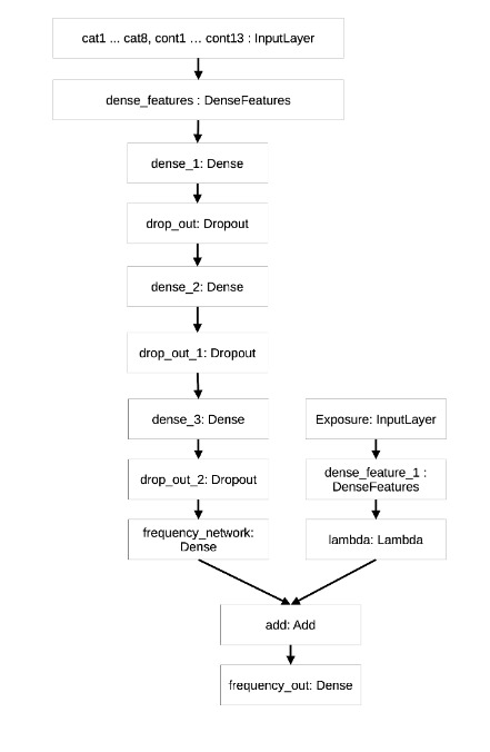
We set the chosen DL architecture by several trials based on previous experiments found in the literature for tabular data analysis (Schelldorfer and Wuthrich 2019; Kuo, Crompton, and Logan 2019). Our approach introduced a dense layer to collect the inputs and handled categorical variables using embedding. Three hidden layers performed feature engineering and knowledge extraction from the input. Dropout layers were added to increase the robustness of the process. As anticipated in the methodological section, the exposure part was handled separately in another branch and then merged in the final layer. The same model structure was used for the CPN, MKT, and TRF models. The TRF model was built first using the pretrained weights calculated on the MKT data and continued the training process on the CPN data in a second step. Figure 7 in Appendix A.8 displays the model structure as exported by the Keras Tensorflow routine.

Overfitting was controlled using an early stopping callback scoring the loss on the validation test and stopping the learning procedure (Zhang and Yu 2005) if the loss was not improved for more than 20 epochs. DL models were trained in Keras Tensorflow 2.4 (Chollet 2018), taking on average 40s per epoch.

4.2.3. Credibility models

For the credibility approach, the original datasets that were in longitudinal format were processed into a wide format (also called unbalanced) needed by the actuar R package (Dutang, Goulet, and Pigeon 2008). Furthermore, as required by the hierarchical Bühlmann-Straub model, continuous variables were discretized using the entire dataset (to have the widest ranges) based on the random forest algorithm. Using the R package ForestDisc (Maïssae 2020), which proposes a random forest discretization approach, we discretized continuous variables into three or four levels by group of variables (cont1–cont2, cont3–cont6, cont7-cont8, cont9–cont10, cont11–cont13) based on their (undisclosed) meaning.

The fitting process of hierarchical credibility models was performed by the cm function of the R package actuar, which allows fitting various forms of credibility models (see, e.g., Goulet et al. (2021)). The response variable used for credibility models was the claim frequency (and not the number of claims). Therefore, predicted claim frequencies were multiplied by exposure to obtain the number of predicted claims.

Several credibility models were compared in terms of performance. We first conducted a simple Bühlmann-Straub model using only the zone_id variable for the three approaches, CPN, MKT, and TRF. Note that for TRF, a new variable entity was created to distinguish the company and market data. This base Bühlmann-Straub model is referred to as BSbase in the following.

Then, we selected the most appropriate HBS model by the most appropriate permutation of categorical explanatory variables cat1–cat8, since there was no particular order among them, except cat1–cat3. More precisely, we considered hierarchical credibility structures as follows cat1, cat2, cat3, then a permutation of cat4, cat5, cat6, cat8, and finally zone_id (and eventually entity for TRF). There were 4!=24 possible HBS models. The best categorical HBS model that minimized the mean squared error when fitting models is referred to as HBScateg in the following.

Finally, we applied the same procedure to select another HBS model using categorical explanatory variables cat1–cat8 and (discretized) continuous variables cont1–cont13. As there were too many (17!) HBS models, we restricted the following hierarchical credibility structures as follows: cat1, cat2, then a permutation of cont5, cont7–10 variables (the most significant continuous variables). There were 5!=120 possible HBS models. The best HBS model is referred to as HBScont in the following.

Given the high number of HBS models fitted and used for prediction on the validation dataset, we used parallel computation using the R (core) package parallel, while model comparisons were performed in an R environment. The running times are summarized in Table 4 and show that MKT and TRF approaches took particularly long to validate. Indeed, fitting time contained only a call to cm() for every HBS model, while validation time made a prediction for every policy of the validation set (see Table 1). The prediction computation was particularly long, but it requires for each policy the exact location in the credibility tree structure starting from the top.

As explained previously, the fitting of HBS models was conducted on the training dataset, the best model (in terms of RMSE) was selected on the validation dataset, and the overall comparison was done on the test dataset.

4.2.4. Performance assessment

The empirical data available for the study faces a risk for which year-to-year loss cost may materially fluctuate due to external conditions (systematic variability) much more than the portfolio risks heterogeneity composition. In this regard, the performance assessment considered not only the discrepancy between actual and predicted losses, but also the ability of the model to rank risks, thereby providing a sensible order of which policies are most prone to suffer a loss in the coverage period. This can be achieved even in contexts where obtaining an acceptable estimate of the pure premium is more challenging (e.g., due to a systematic unmodeled social or environmental trend in either frequency or in severity). The ability of ML to identify nonlinear patterns and interactions is useful both to model the pure premium and to rank risks.

To compare the credibility and ML models within or between model classes, we used the NGI, the ratio between the sum of observed claims and the sum of expected claims (denoted by actual to predicted ratio), the MAE, and the RMSE. The NGI is a discriminant metric that ranks models according to their ability to predict, while the actual to predicted ratio is used to check whether the model is generally unbiased on a total basis. For both metrics, the closer to one the metric is, the better the model is. MAE and RMSE measure the overall distance between observations and predictions. Best models are identified by the lowest values.

The choice of models deserves a final consideration. The RMSE and NGI indices typically move in the same direction, so minimizing the prediction error, which is the pivotal objective of risk pricing, also means maximizing the model’s discriminating ability, which may be of greater underwriting or marketing interest. If this is not possible, the analyst will rely on either the first or the second metric depending on the business context. Finally, the availability of tools to interpret models should be considered; indeed, it may become an essential selection criterion in some contexts where the ability to explain a model is essential for regulatory or marketing purposes.

4.3. Interpretation and predictive performance of model results

This section focuses on interpreting the ML and credibility models. We examined variable importance for ML models and analyzed credibility factor densities related to the best HBS models. In a second step, we assessed performance of both approaches.

4.3.1. Model interpretation for ML

ML models have long been considered black boxes, but methods have been developed to provide explanations of model structure and provide outputs, even in actuarial science (see, e.g., Lorentzen and Mayer (2020)). In our application, we simply focused on the variable importance analysis internally calculated by the LightGBM model. That measure of variable importance broadly reflects the gain of using that feature in LightGBM trees to reduce training losses. Variable importance analysis in DL models is not automatically calculated during the training stage and requires the use of a separate algorithm (e.g., one with Shapley values (SHAP); Lundberg and Lee 2017), which is outside the scope of this paper. Another possible approach would be to use permutation importance, but there are no readily available routines for Tensorflow datasets. However, it is reasonable to assume that variable ranking is similar between the two ML approaches.

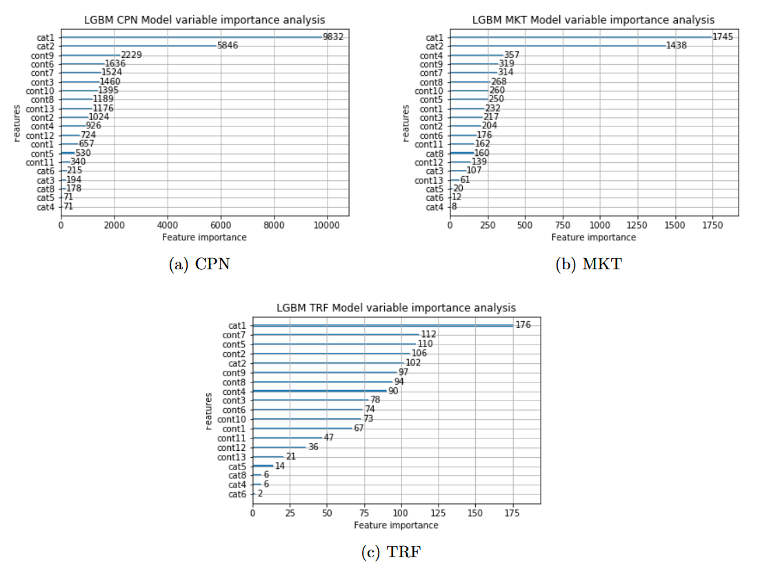
Figure 4 displays LightGBM for the CPN, MKT, and TRF approaches. The following considerations can be drawn:

1. The cat1 and cat2 variables are consistently ranked as the most important predictors both for MKT and CPN approaches, as shown in Subfigures 4a and 4b.

2. The TRF plot, Subfigure 4c, is more difficult to interpret. It indicates which variables most likely correct the difference between the MKT and CPN models. While cat1 keeps first place, the relative importance of other variables is higher than in the MKT and CPN plots.

Figure 4.LightBM variable importance for CPN, MKT, and TRF approaches.

By construction, the ML models used here are black box and require post hoc interpretability tools to analyze the effect of features. Given the anonymous nature of the data, we limited ourselves to an illustration of the overall interpretability of the variables, which allows an actuary to understand the overall effect of variables on the tariff. Depending on the audience involved in the interpretability analysis (Delcaillau et al. 2022) (e.g., an actuary or a policyholder interested in its tariff), it may be necessary to discuss in depth the local interpretability and variable interaction issues.

4.3.2. Model interpretation for credibility

The approach we used to select the best HBS model was based on permutations, which implicitly accounts for the importance of variables when building the hierarchical tree structure. Therefore, the structure of the best HBS model selected in Table 4 can be compared with variable importance results depicted previously. We note in particular the role of the variables cat1 and cat2, whose importance remains unchanged for MKT and CPN approaches. The cat2 variable also stands out significantly for the TRF approach, which is not the case with the LightGBM model.

Additionally, Figure 5 displays the empirical distributions of fitted credibility factors for the best HBS model with categorical variables for the three approaches (CPN, MKT, TRF). Recall that the higher the probability of the coefficient being close to one, the more significant the variable is in the construction of the hierarchical tree. For both CPN and MKT, Subfigures 5a and 5b, we observe higher credibility factors for the same variables, cat2, cat3, and the third variable in the hierarchical structure. Whereas for TRF, Subfigure 5c, lower credibility factors were fitted even for cat2 and cat3.

These analyses provide an empirical approach to globally measure the importance of variables on the tariff. Unlike a black box model, these analyses are directly derived from the model structure. In addition, its hierarchical structure and the value of the credibility coefficients allow us to visualize the decision process of the algorithm and the resulting local predictions similar to a decision tree. The HBS model is therefore easily interpretable and transparent.

However, this approach to interpreting the HBS model is constrained by the choice of a credibility-based approach, which depends on the claims history of the policyholder. From this viewpoint, the model predictions do not necessarily depend only on a variable’s importance, but also depend on the experience accumulated in the claims history. In some situations, the seniority of the claim is not important; recent information may better represent the current nature of the risk. Further research is needed to develop indicators that would distinguish the relationship between variables, their effect on the rate, and the importance of past experience in a credibility framework.

Figure 5.Empirical densities of credibility factors of the best HBS models.

4.3.3. Predictive performance analysis

Table 5 reports the predictive performance, evaluated on the company test set, for the DL, light gradient boosting, and credibility models, whereas Figure 6 displays the normalized NGI against other metrics for each model point. The column Approach indicates whether the model is trained on market only (MKT), company only (CPN), or company data using a transfer learning approach (TRF). Again, we stress that the predictive performance analyses of the different approaches were conducted on the (same) test company dataset to ensure comparability.

Figure 6.Normalized Gini (NGI) against other metrics.

First, the actual/predicted ratio was between 0.9 and 1.1 for all models, but as expected, CPN’s was the worst. This result was indeed expected since the MKT dataset includes the company’s data. We anticipated that since the test set considers a different year than the training and validation sets, the predictions may be structurally biased because the insured risk strongly depends on the year’s context, and frequency trending is not considered in the modeling framework at all. Nevertheless, the results show that the MKT data, in this case, provided a superior experience compared with the CPN only data.

The LightGBM model results showed the best performance with the TRF and MKT approaches when measured by the NGI and MAE. We also noted that the LightGBM with the TRF approach was the best model in terms of RMSE. The HBS model built with categorical explanatory variables performed well with the MKT approach and was the second or third best model, depending on the metric considered. Given its nonparametric nature, this model is very flexible for adjusting to different feature effects. We generally observed that combining company data with external market data had a significant advantage in predictive performance for both the ML and credibility models. However, only the LightGBM model seemed able to exploit the TRF approach in an appropriate way. Indeed, it seems that the TRF approach penalized the credibility methods, which can be explained by a more important weight given to the information related to the company.

Regarding the predictive accuracy, especially for the DL models, we cannot rule out that the superiority of TRF approaches holds for all possible ML architectures.

5. Conclusion

Credibility theory is widely used in actuarial science to enhance an insurer’s rating experience. In particular, hierarchical models account for the effect of different covariates on the premium by splitting the portfolio into different levels. Hierarchical models are easily interpretable and provide actuaries with a clear picture of the pricing process by classifying policyholders according to their risk and claim history. However, they are not very flexible and make it difficult to capture nonlinearities or interaction effects between variables.

In this paper, we present an application of ML methods, the LightGBM model and a deep learning model, which can be compared with the hierarchical credibility approach to transfer the experience applied on a different, but similar, book of business to a newer one. Two approaches for each model were examined: the first directly applied an ML model pretrained on market data, while the second relied on transfer learning logic, where the pretrained model was fitted on the insurer’s data. We performed our empirical analysis transferring loss experience from an external insurance bureau to a specific company portfolio. We focused on the global predictive performance and not individual features or cluster of exposures (e.g., zone_id) due to the anonymized format of the data. Our approach allowed us to significantly improve the prediction performance of an ML model compared with a model only trained on the insurer’s data. Our results show the advantage and efficiency of pretraining an ML model on a reference dataset. We also observed that HBS models performed well on market data or company data alone in our application, indicating that the transfer does not improve the prediction power compared with the MKT or the CPN approaches, depending on the chosen metrics (MAE or RMSE). Finally, ML approaches obtained more competitive results compared with credibility models with this dataset. However, it is reasonable to expect that as the company data increases, the advantage of the MKT and TRF approaches decreases with respect to a model trained only on company data.

Hierarchical credibility and ML models are flexible enough to handle other types of data or business in insurance applications when reference data are available. The only disadvantage is the training validation test computation time, which might be too long for big datasets. However, applying MKT or TRF approaches should be transposed to a specific context by replacing a market/company situation with, for example, a holding group/entity or company/line of business situation, because, in practice, the loss experience of competitors remains unknown. ML models also have a practical advantage in that their implementation is relatively automated, while HBS model implementation may require a manual and expensive selection phase to derive the best feature combinations. Moreover, the code to train an ML model, as shown in this or similar studies, is readily available (see, e.g., Appendix A.3) and can be replicated on an adequately resourced PC without too much effort.

This technique can be used to rate many insurance products. Although our exercise applied it to agricultural insurance, in theory it can be applied to any insurance industry context where the set of ratemaking variables shared between two distinct portfolios is nonempty, holding the common ratemaking variables in the same domain between the two portfolios. First, the transfer of experience may be performed within the same company, for example, when new products, tailored for niche lines of business, are created. Initial loss estimates may be performed on the initial product and then applied as initial scores to the newer portfolio. A second application can be considered in reinsurance.

The nature of their business allows reinsurance companies to underwrite similar risks from different primary insurers. Often, a small proportional treaty is the way to fully overview the loss experience of a new underwritten portfolio. When setting the reinsurance cover or when assisting their clients to set rates for new covers or new markets, the need to blend individual and market experiences emerges, so that reinsurers can make benchmark datasets for training ML models. However, in non-life insurance, it will be necessary to ensure that these benchmarks contain characteristics comparable to those of the insurance product being priced, in order to properly extrapolate the results, as previously anticipated.

Nevertheless, the models applied in this paper can be improved. The HBS models we used need categorical variables, which led us to categorize continuous variables, thereby losing information. It is an open question whether regression credibility’s Hachemeister models could improve predictions. In addition, the computational performance of HBS models is challenging for actuaries with large insurance portfolios. For example, future research could focus on improving the variable selection process, which is currently cumbersome, although the model is based on an explicit formula. Finally, future work can explore how to interpret the marginal effect of explanatory variables in credibility models. A possible direction may include developing summary indicators based on credibility models to assess the feature importance and role of policyholder’s experience.

These connections between credibility theory and ML techniques open pathways for future research. We used an empirical approach to build the hierarchical tree structure of the credibility model. One way to improve this is to define the tree structure through different partitioning tree models, similar to Diao and Weng (2019), where the partitioning algorithm directly includes credibility theory. From there, it is natural to consider that such a credibility regression tree can be applied to other ensemble decision tree algorithms, such as boosted trees. It would be interesting to measure the interest of an approach based on transfer learning on this type of model.

6. Acknowledgments

The authors wish to give a special thanks to CAS research and publications staff for their support.

The authors are also very grateful for the useful suggestions of the two anonymous referees, which led to significant improvements of this article. The remaining errors, of course, should be attributed to the authors alone.

This paper also benefits from fruitful discussions with members of the French chairs DIALog (digital insurance and long-term risks) and RE2A (emerging or atypical risks in insurance), two joint initiatives under the aegis of the Fondation du Risque.