Claim Reserving: Performance Testing and the Control Cycle

undefined

1. Introduction

Fundamentally, estimates of claim liabilities are predictions or forecasts. Presented with a body of historical data, and with knowledge of the operation of the business and the exposures underwritten, the actuary is called upon to develop a forecast of the future cash flows associated with the settlement of all unpaid claim obligations. Since claim development involves one or more underlying stochastic processes, the actuary must separate noise from signal in the available data. This necessitates the selection of an underlying model, application of the model to the available data, selection of model parameters, and interpretation of the results. The resulting forecast will be subject to estimation errors resulting from both any misspecification of the model and misestimation of its parameters, as well as random process variation.

Typically the actuary will employ several actuarial projection methods and select an actuarial central estimate of the claim liabilities after reviewing the results of each method, giving appropriate weight to the indication produced by each method and supplementing the mechanically generated indications with judgment. A natural question to ask of the actuary is, “How do you know that the methods chosen are the most appropriate ones to employ?” A corollary question is, “How do you decide the relative weight to be given to the results from each method?” While some might reply that the selection of methods and the assignment of weights are actuarial judgments made with the benefit of experience, in the current regulatory and accounting environment there is a need to respond with greater clarity to such questions. It therefore seems worthwhile to develop a formal methodology to assess the accuracy of the methods used to make actuarial estimates.

Ongoing performance testing of methods can help (a) provide empirical evidence as to the inherent level of estimation error associated with any particular method; (b) provide insight into the strengths and weaknesses of various methods in particular circumstances; (c) provide assurance that the actuary is using the best methods for the given circumstance; (d) provide useful information regarding the appropriate weights to be given to each method; and (e) ultimately lead to meaningful improvements in actuarial estimates, in the sense of lower estimation errors, as the stronger methods win out over the weaker methods, based on objective evidence as to their performance.

Performance testing can also assist in managing the potential overconfidence of the actuary, a topic discussed by Conger and Lowe (2003). Behavioral scientists have demonstrated that the vast majority of managers are overconfident in their ability to make accurate forecasts—of everything from estimates of next year’s sales revenue, to the cost of implementing a new system, to the delivery date of a new product under development—because they lack meta-knowledge about the limitations of their forecasting abilities.^[1] Overconfidence is a problem because blown estimates, cost overruns, and missed deadlines hurt business performance. Actuaries are not immune to the overconfidence phenomenon; it manifests itself when actual claims are outside the range more frequently than expected. The formal feedback loop provided by the control cycle helps the actuary develop this metaknowledge, becoming “well-calibrated” as to the true limitations of his or her actuarial projections.

In addition to improving the quality of the actuarial estimates of claim liabilities, performance testing results are also useful in other contexts such as setting ranges around central estimates and measuring required economic capital for reserve risk.

Since estimates of claim liabilities are forecasts, performance testing of actuarial projection methods should involve proper measurement of prediction errors via a standard statistical technique, referred to as cross-validation. This paper provides an overview of cross-validation, defines how it would be employed in the context of property and casualty claim liability estimates as a key element of the control cycle, and provides some illustrative empirical results.

Including this introduction, this paper is organized into four sections. Section 2 of the paper lays out a definitional framework for claim liabilities and the actuarial estimation process. Section 3 discusses performance testing in general, including performance criteria and crossvalidation techniques; and introduces the actuarial control cycle, outlining the role that performance testing should play in it. Section 4 illustrates all of the concepts via a case study, using real data from a U.S. insurer, with additional calculation details provided in an Appendix.

The case study generates some interesting conclusions, highlighted here to pique the reader’s curiosity.

• At some maturities, a method that projects the ultimate claim liabilities from the outstanding case reserves outperforms the reported chainladder method.

• Ultimate claim counts can be predicted with much greater accuracy than ultimate dollars. This implies that projection methods that make use of claim counts can be more predictive than those that do not. While the greater stability of claim count projections may be partially offset by greater instability of average claim values, the information value of the claim counts should lead to a net improvement in overall accuracy over projections that ignore claim count information.

• Methods that formally adjust for changing settlement rates or case reserve adequacy have greater predictive accuracy than the analogous methods applied without adjustments. When changes in claim settlement rates and/or changes in case reserve adequacy occur, the accuracy of projection methods that do not adjust for them is materially degraded.

• In assessing which projection methods to employ, and how to combine the results from several methods, the degree of correlation between the estimation errors is an important consideration. To illustrate, if the results of two methods are perfectly correlated but the estimation errors from one are twice the estimation errors of the other, then the appropriate course of action is to drop the method with the higher estimation errors entirely. A different course of action would be implied if the errors were uncorrelated.

Not all of the conclusions from the case study can be generalized beyond its immediate circumstances. However, the case study does demonstrate the kinds of insights that can be obtained through the performance testing process, and the utility of those insights in the control cycle. Performance tests that we have performed on other lines of business and other actuarial projection methods also confirm the value of the exercise, suggesting that this is a fertile field of empirical investigation. The authors would encourage others to pick up where the paper leaves off and add to the body of performance testing research.

2. Defining the claim liability estimation process

Before describing performance testing, it is necessary to establish a definitional framework for the process by which claim liabilities are estimated.

2.1. Claim liabilities

Claim liabilities are the loss and loss adjustment expense obligations arising from coverage provided under insurance or reinsurance contracts. The term may refer either to actual claim liabilities (that is, an after-the-fact realization of the claim payments) or to estimated claim liabilities produced by an actuarial projection method.

Claim liabilities may be estimated either on a nominal basis or on a present value basis. While estimates are more commonly made on a nominal basis, estimates on a present value basis are more representational of the economic cost of the claims. Present value estimates may be less accurate due to misestimation of the timing of payments; they also may be more accurate because the predicted payments further into the future—which are subject to the greatest uncertainty—are given successively less weight.

Let $C_{i, d}$ represent the actual incremental paid claims on the ith accident year^[2] during the dth development period. Claim development is the realization of the actual claim liabilities, $C_{i, d}$, over time, reflecting the confluence of a number of underlying stochastic processes: claim generation, claim reporting, claim adjusting, and claim settlement. (On a net basis, additional processes would include the identification, pursuit, and recovery of subrogation, salvage, third-party deductibles, and reinsurance.)

Since they are the result of stochastic processes, all $C_{i, d}$ are random variables.

We typically have a triangular array of actual values of $C_{i, d}$, up to the current calendar point in time t = i + d – 1, as shown below.^[3]

$$\left[\begin{array}{lllll} C_{1,1} & C_{1,2} & C_{1,3} & C_{1,4} & C_{1,5} \\ C_{2,1} & C_{2,2} & C_{2,3} & C_{2,4} & \\ C_{3,1} & C_{3,2} & C_{3,3} & & \\ C_{4,1} & C_{4,2} & & & \\ C_{5,1} & & & & \end{array}\right]$$

These actual $C_{i, d}$ are a sample partial realization from the underlying stochastic processes.

Let $\hat{C}_{i d}^{(t)}$ represent^[4] the estimate (more accurately, a forecast) of the expected incremental paid claims on accident year i during development period d, based on information at time t.

The actual aggregate discounted claim liabilities at time t are given by

$$L^{(t)}=\sum\left(v_{i+d}\right)\left(C_{i, d}^{(t)}\right) \quad \text { for all } \quad i+d-1>t, \tag{2.1}$$

and the estimated aggregate discounted claim liabilities at time t are given by:

$$\hat{L}^{(t)}=\sum\left(v_{i+d}\right)\left(\hat{C}_{i, d}^{(t)}\right) \quad \text { for all } \quad i+d-1>t, \tag{2.2}$$

where $v_{i+a}$ is the discount factor applicable to payments made i + d – t periods after t.

Finally, actual and estimated aggregate claim liabilities are related by

$$L^{(t)}=\hat{L}^{(t)}-e \tag{2.3}$$

where e is the estimation error, the difference between the estimated and the actual realization of the claim liabilities. Because all of the $C_{i, d}$ are random variables, e is also a random variable.

$\hat{L}^{(t)}$ may be broken down into component estimates; for example, the estimated liabilities associated with a particular accident year, or the liabilities that are expected to be paid in a particular future calendar year. Because they are estimates of means, the total of the component estimates is equal to the overall estimate, $\hat{L}^{(t)}$.

In contrast to claim liabilities, a claim reserve is a balance sheet provision for the estimated claim liabilities at a particular statement date. The reserve is a fixed, observable, known quantity, not an estimate. Those who speak of “reserve estimates” are guilty of sloppy language, which hopefully does not translate into sloppy thinking. The reserve is a financial representation of the underlying obligations, reflecting the valuation standards associated with the particular financial statement of which it is an element. These standards are established by the applicable regulatory and accounting bodies within the jurisdiction. Such valuation requirements might not equate the reserve, $R^{(t)}$, with the associated estimated liabilities, $\hat{L}^{(t)}$. For example, regulatory requirements might stipulate that the reserve be set conservatively at a percentile above the mean. Alternatively, the reserve might include a margin for the cost of the economic capital required to support the risk of the associated claim liabilities. It is sufficient for our purposes to simply note that $R^{(t)}$ = f($\hat{L}^{(t)}$), (or more precisely the distribution around $\hat{L}^{(t)}$) where f is determined by the particular regulatory/accounting regime.

2.2. Actuarial projection methods

An Actuarial Projection Method is a systematic process for estimating claim liabilities. It encompasses three fundamental elements:

• An algorithm, which is used to project future emergence and development. Any algorithm is predicated on an underlying model, which is a mathematical representation that embodies explicit and/or inferred properties of the claim incidence, reporting, and settlement processes; the algorithm applies the model to a given dataset to produce an estimate of the claim liabilities.

• A predictor dataset, which is the input data used by the method. Specification of the dataset includes the types of data elements, the valuation points of those data elements that vary over time, and the level of detail at which the projection is performed (for example, separate analyses for indemnity and expense, or by type of claim, class of policyholder, or jurisdiction). The dataset may include data external to the entity in addition to internal data; it may also include qualitative information as well as quantitative.

• Intervention points, which are points in the process at which judgments are made by the actuary. These include the selection of assumptions (model parameters such as chain-ladder link ratios), overrides to outlier data points, and other adjustments from what would otherwise be produced by mechanically applying the algorithm to the data.

A particular method m(a,d,p) (i.e., consisting of an algorithm, a dataset, and intervention points) is selected by the actuary from the set of all possible methods M(A,D,P) to produce an estimate of the claim liabilities, $\hat{L}^{(t)}_{m}$, at a valuation point t, for example at the end of a given calendar year.

A projection method might use data with a valuation date that is earlier than the valuation date of the estimated liabilities; in such a case the actuarial projection method would include the “roll forward” procedure that adjusts for the effects of the timing difference.

Most traditional projection methods assume stationarity of the underlying claim processes, such that the historical development in the dataset is assumed to be representative of the conditions that will drive the future development. Often this is not the case, and the data must first be adjusted to reflect the current and anticipated future conditions. Such adjustments, when made, are part of the actuarial projection method.^[5]

Wacek (2007) distinguishes between clinical predictions, which are conclusions reached by an expert when presented with a set of facts about a problem of a type with which he or she has experience; and statistical predictions, which are conclusions indicated by a quantitative or statistical formula or model using a set of quantifiable facts about a problem. He points out that an expert making a clinical prediction may use a statistical model, but if the model results are augmented by consideration of other information and the judgment of the expert, then the prediction would be classified as clinical. Thus the estimation of claim liabilities is generally a clinical rather than a statistical prediction. The inclusion of intervention points in the definition of an actuarial projection method is in recognition of the important role that endogenous information and judgment play. All statistical prediction models/methods have inherent limitations; many of those limitations are routinely addressed by the actuary through the use of intervention points and the insertion of judgment into the estimate.

Performance testing can be done on either statistical predictions (those involving a mechanical application of the algorithm without any judgmental interventions) or on clinical predictions in which we are testing the actuary’s performance, not just “the machine’s” performance.

2.3. From actuarial projections to the actuarial central estimate

Ultimately, the actuary is responsible for developing an actuarial central estimate of unpaid claim liabilities, representing an expected value over the range of reasonably possible outcomes. In developing an actuarial central estimate, the actuary will typically use multiple actuarial projection methods that rely on different data^[6] and require different assumptions. For each method employed, the actuary can produce alternative actuarial estimates by varying the selected parameters and other judgments made at the intervention points in the method. Ultimately, the actuary will settle on parameters and assumptions that produce the central estimate for each method.

One can view the central estimate from each method as a sample mean, developed from a sample of the data. Each sample mean will have a sample variance, depending on the predictive quality of the sample data employed. The actuary will reconcile/combine the sample means by assigning a relative weight to each one to produce the actuarial central estimate.

3. Performance testing and the control cycle

Within the definitional framework articulated in the previous section, we can now turn to the problem at hand.

The first issue facing the actuary is to choose a finite set of actuarial projection methods {m₁, m₂, . . . m_n} from the set of all possible methods M that is “best” for a particular class of business and circumstance.^[7] The second issue is to combine the results of the individual methods together into a single estimate that is “best,” giving appropriate weight to each method based on its predictive value in the specific circumstances. As will be seen in subsequent sections, both issues can be addressed more formally via performance testing.

3.1. Performance testing and selection of methods

In establishing a performance testing methodology, one needs to start by establishing appropriate performance criteria. In other words, by what set of criteria do we say that one method is better than another? Preference for one method over another would then be based on performance test results against those criteria in the specific circumstances.

Obviously, the choices of methods at a given point will also be constrained by the available data (both quantity and type) and the available resources to produce and analyze them. However, over time, performance testing can assist in evaluating the benefits against the costs of generating currently unavailable data elements or of adding resources to support more labor-intensive projection methods. Performance testing might even reduce actuarial resource costs by redeploying resources away from actuarial methods that do not meet cost-benefit criteria.

Statisticians and forecasters traditionally argue that the best method is the one that produces estimates that are unbiased and minimize the expected squared error. Such methods are described as “BLUE”—Best Least-Square, Unbiased Estimators.

For our purposes, we extend the criteria somewhat beyond BLUE. In evaluating the performance of actuarial projection methods it is appropriate to consider the criteria listed in Table 1.

Our criteria extend the acronym from BLUE to “BLURS-ICE”—Best Least-Square, Unbiased, Responsive, Stable, Independent, and Comprehensive Estimate.

The minimum squared error criterion is obviously the strongest; it is the primary yardstick against which methods are compared. The requirement for unbiased estimates is a weaker criterion, in that we would accept methods with bias if the bias were measurable or immaterial. In other words, we would be willing to trade a lower expected squared error for the introduction of a manageable level of bias. Stability and responsiveness are desirable characteristics, but are also weaker criteria.

Comprehensiveness and independence look at the problem through a slightly different lens than the other criteria. These two criteria relate to the issue of combining multiple estimates together to obtain an actuarial central estimate. The comprehensive criterion stems from our desire to maximize the information value of all of the available data; rather than applying many separate methods to disparate data elements it is preferable to use fewer, more comprehensive methods. Similarly, the independence criterion stems from a desire to not waste resources on methods with highly correlated estimation errors, producing essentially the same answer as another method. If the errors from two projection methods are highly correlated it is preferable to eliminate the one with the higher expected squared error.

3.2. Performance testing using cross-validation

Rather than invent a performance testing methodology from scratch, we need only look to the approaches used in other sciences that are also called upon to make forecasts. Statistical techniques to measure the accuracy of forecast models are abundant in the literature of other professions. For example, as a result of the ongoing interest in hurricanes, the authors have had occasion to review the literature relating to the accuracy of hurricane forecasts made by climatologists. In climatology, the “skill” of statistical forecasting methods is measured via cross-validation. The method of cross-validation is outlined in Michaelson (1987). The validity of the method for estimating forecast skill is discussed in Barnston and van den Dool (1993). The potential pitfalls and misapplication of the method are discussed in Elsner and Schmertmann (1994).

Cross-validation, properly applied, permits a fair comparison of the skill of competing forecast models. For example, forecasts of the expected number of major hurricanes spawned in the Atlantic basin are made annually by Gray and Klotzbach (2008) and others, based on statistical models that relate the level of Atlantic hurricane activity to other climate variables such as the state of the El Niño Southern Oscillation (ENSO) in the Pacific. The skill of each of these models can easily be measured and compared via crossvalidation. Similar cross-validation tests are performed to measure the skill of storm path forecast models employed by the National Hurricane Center. This helps users of the forecasts to appreciate their limitations, and allows each modeler to place formal ranges around the central estimate of their model’s forecast. It also facilitates the selection of the “best” forecast model and provides direction to the course of further research and enhancements.

Cross-validation is a straightforward, nonparametric approach to estimating the errors associated with any forecast produced by a model. This would include forecasts of future claim payments in estimating claim liabilities. Cross-validation is relatively simple to implement, given sufficient data. It is quite general in its applicability to any suitable defined actuarial projection method, and has intuitive appeal because it closely mimics the actual claim liability estimation process.

3.3. Cross-validation in general

The basic approach in the context of a general statistical forecasting model is to develop a model using all observations except one, and then to use the model to produce a forecast of the omitted observation. This process is repeated iteratively, generating a forecast from a new model developed by excluding a different observation each time. The cross-validation exercise generates an independent forecast for each observation, based on a model generated by the rest of the data. The skill of the model can then be measured by comparison of the forecasts to the actual outcomes.

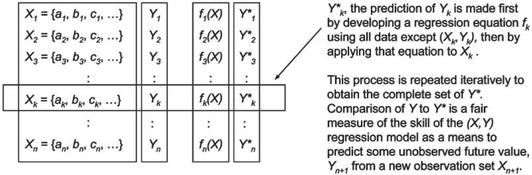
For example, let Y represent a random variable that we believe is dependent on some set of independent variables X = {a, b, c, . . .}. In other words we believe that Y = f(X), although we don’t know the precise form of f. Suppose that we have n historical observations of (X,Y), and would like to develop a linear regression model that predicts future values of Y given X. Rather than using all n values of (X,Y) to develop the regression equation, the cross-validation approach would develop n regression equations, each one based on n – 1 of the observations. Each equation would then be used to predict the Y value of the excluded observation, Y∗, as displayed schematically in Figure 1.

Comparison of the actual values of Y to the predicted values Y∗ is a fair way to measure the true ability of a linear regression model to predict Y from X. We are testing the predictive ability of a linear model, not the parameters of the model itself. By comparison, the standard error of the regression is not a fair way to measure the equation’s predictive ability. The standard error is a measure of the degree to which the equation explains the variation in Y; inevitably the standard error of a regression overstates predictive ability because, in finding the best-fit equation to the data by minimizing the errors, the result inadvertently “explains” some of the noise in addition to the signal in the sample data.

Once the cross-validation tests have been performed, then all of the data can be used to develop the best regression model for use in predicting ${Y}_{n+1}$.

Elsner and Schmertmann (1994) point out that the form of the equation, as well as the parameters, must be incorporated into the cross-validation test for it to be fair. Going back to our regression example, let us assume that in developing our regression equation some of the variables in the set X might not be significant, or might create problems of autocorrelation, such that the final regression equation might make use of only a subset of the variables in X. It would not be fair to use all of the data to decide which variables to retain and which to eliminate, and then perform cross-validation on the data with the selected equation. Instead one must start with all of the variables and go through the process of elimination in developing each of the n equations for the cross-validation test to be fair. Cross-validation properly performed, captures model risk as well as parameter and process risk.

Also, in designing the test it is important to consider whether using data on “both sides” of each (X,Y) value will result in a fair test. Suppose that the data is a time series—for example, the numbers of Atlantic hurricanes occurring in each calendar year over a 20-year period. In the general case, we would use 20 observation sets of 19 data points to develop 20 forecasts that could be compared to the actual values. This would include using observations from years after a particular year to forecast the results for that year. Of course, in reality the subsequent observations would not have been available at the time we were making the forecast. This is only a serious problem if the data exhibits serial correlation, typically due to a trend, cyclicality, or other nonstationary situation. Where serial correlation is present in time-series data, using adjacent data on both sides provides too much information about the omitted value to the forecast model; in such situations sufficient adjacent data points on one side should be excluded so that the test is fair. Where serial correlation is not present, the observations can be treated as a sample set without order significance. This issue is particularly relevant in the context of performance testing of claim liability estimates, as there is very little data in insurance that does not exhibit serial correlation.

The cross-validation approach goes by a variety of other names, depending on the context. Those involved in developing predictive statistical models might refer to the approach as testing the model using out-of-sample data. Meteorologists refer to cross-validation as “hindcast” testing. In the context of claim liability estimation, some actuaries refer to it as retrospective testing.

3.4. Application of cross-validation to estimates of claim liabilities

The cross-validation approach applies quite naturally to the estimation of claim liabilities. It can be applied to an overall actuarial method, used to develop $\hat{L}^{(t)}_{m}$; or to a component of the method—for example, one that estimates the claim liabilities for an accident year at a particular maturity, or one that forecasts the expected incremental claim payments for an accident year in a particular development year.

One issue with cross-validation in a claim liability estimation context is whether any data after a point in time can be used to validate estimates of claims before that point in time. As was discussed in the previous section, cross-validation tests require careful design to assure that they fairly assess predictive skill.

In the context of testing an actuarial projection method, the selected actuarial projection method is typically applied to a historical dataset that is limited to information that would have been available at the time, and the resulting estimate of the claim liabilities is compared to the actual outcome with the benefit of hindsight reflecting the actual run-off experience. This assures that the test is a realistic and fair test of the performance of the method. The dataset is then brought forward to the next valuation point, and the estimation process is repeated. Schedule P of the U.S. Annual Statement includes this type of cross-validation test of the historical held reserves.

We illustrate the application of the standard performance testing technique in the case study in Section 4, with additional calculation details in the Appendix.

Finally, we note that in most actuarial projection applications one does not have the luxury of knowing the actual value of the claim liabilities, ${L}^{(t)}$, because the subsequent run-off is not complete. Instead, one typically only knows the actual run-off through the current valuation point, and must combine it with the current actuarial central estimate of any remaining unpaid claim liabilities to obtain a proxy for ${L}^{(t)}$. This is a practical concession that one must make unless one is prepared to restrict the analysis to very old experience. The validity of the results is a function of the proportion of each “actual” value that is paid versus still estimated unpaid, statistics that should be tracked throughout the analysis. A final step in each performance test exercise will be to be sure that the results and conclusions are not unduly influenced by the current estimates of the remaining liabilities.

3.5. Performance testing as an element of the reserving control cycle

The importance of an actuarial control cycle has been presented by many others. The concept was first presented by Goford (1985) in an address to U.K. actuarial students in the context of life insurance. Since then, the actuarial control cycle has been adopted as an educational paradigm by many actuarial organizations, most notably the Institute of Actuaries in Australia. Most recently, the Casualty Actuarial Society has announced a major revision to its basic education and examination structure, one element of which is the addition of the actuarial control cycle to the new Internet-based exam modules [see for example, Hadidi (2008)]. For a general introduction to the Control Cycle see Bellis, Shepherd, and Lyon (2003).

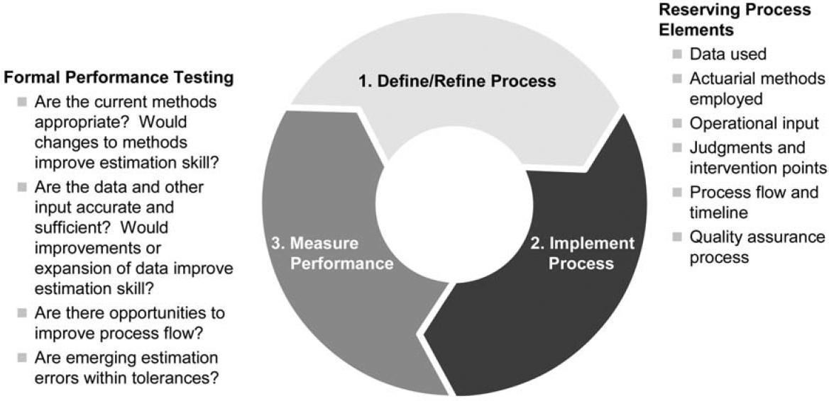
In the context of loss reserving a control cycle involves identifying, testing, and validating all elements of the process by which claim liabilities are estimated. Figure 2 depicts what the control cycle might look like in this context. Most importantly the control cycle should involve an ongoing assessment of the estimation skill of the actuarial methods currently being employed, and exploration of opportunities to enhance overall estimation skill by implementing better actuarial projection methods, based on all of the BLURS—ICE criteria. As with other control cycles, the reserving control cycle is critical to the management of reserve risk.

Those with an engineering background will recognize that the actuarial control cycle is a specific application of a more general approach to quality assurance and continuous process improvement. Periodically, in a planned manner, one steps back from the production process to assess its effectiveness and to identify ways to improve it. The control cycle also codifies that, in addition to a production role, the actuary has a developmental role to play. This latter role can often get lost in the crush of production activities.

In the reserving control cycle, performance testing is the primary assessment tool. As part of the control cycle, the actuary would identify those areas where the greatest exposure to estimation errors is present, and seek process improvements to mitigate the exposure to those errors. This can take the form of improvements in the quality, timeliness, and range of data relating to the nature of the underlying exposures and emerging claims, or the introduction of new actuarial projection methods that make use of new data or better leverage existing data. Occasionally it will take the form of changes to people or systems involved in the claim reserving process.

Implementing performance testing within the claim reserving control cycle can be labor intensive, especially initially when the process is first being established. It is impractical to expect that extensive performance tests would be performed on every possible actuarial method for each class of business, with the detailed analysis updated during every reserving cycle. Fortunately, this is not necessary. Insights gained from the analysis of one class of business often extend to other similar classes. And, since the additional insight gained by updating the data with one new diagonal is incremental, the annual updates for each class do not entail an extensive analysis.

Performance testing can be substantially facilitated by capturing the central estimate from each actuarial projection method, along with the final selected actuarial central estimate, for each class of business in a relational database on an ongoing basis. Reconstructing this information after the fact can be a substantial archaeological exercise, particularly when the methods involve intervention points with judgmental selections. Reconstruction exercises are often necessary to “seed” the database initially; the database is then updated with new projection results on an ongoing basis. Once this database is established, ongoing performance test results for existing methods can be produced somewhat mechanically. Obviously this will not be the case for new actuarial projection methods, where some “back-casting” of the method is necessary to get an initial view of its performance.

The key to successful implementation of performance testing within the control cycle is a carefully-thought-out test plan that focuses on a few key issues and experiments with a few new methods or new data sources.

4. Illustrative case study

In this section, we move the discussion from concept to practice, by means of a real-world case study based on the actual reserving experience of a major U.S. insurer. While we draw some actual conclusions from the case study, its primary purpose is to illustrate the application of performance testing, cross-validation, and the control cycle. While our work in this area (including performance testing on other datasets) generally confirms the findings in the case study, we can’t say that all of the conclusions drawn from the case study can be generalized to other companies or circumstances.

4.1. The company and its data

The case study is based on the experience of a company that no longer exists in its historical form, having been transformed by a series of subsequent mergers and acquisitions. Since the company was a long-standing client of the authors’ firm, a wealth of historical reserving experience is available. We are appreciative of the successor company’s support in allowing us to publish results based on the historical dataset.

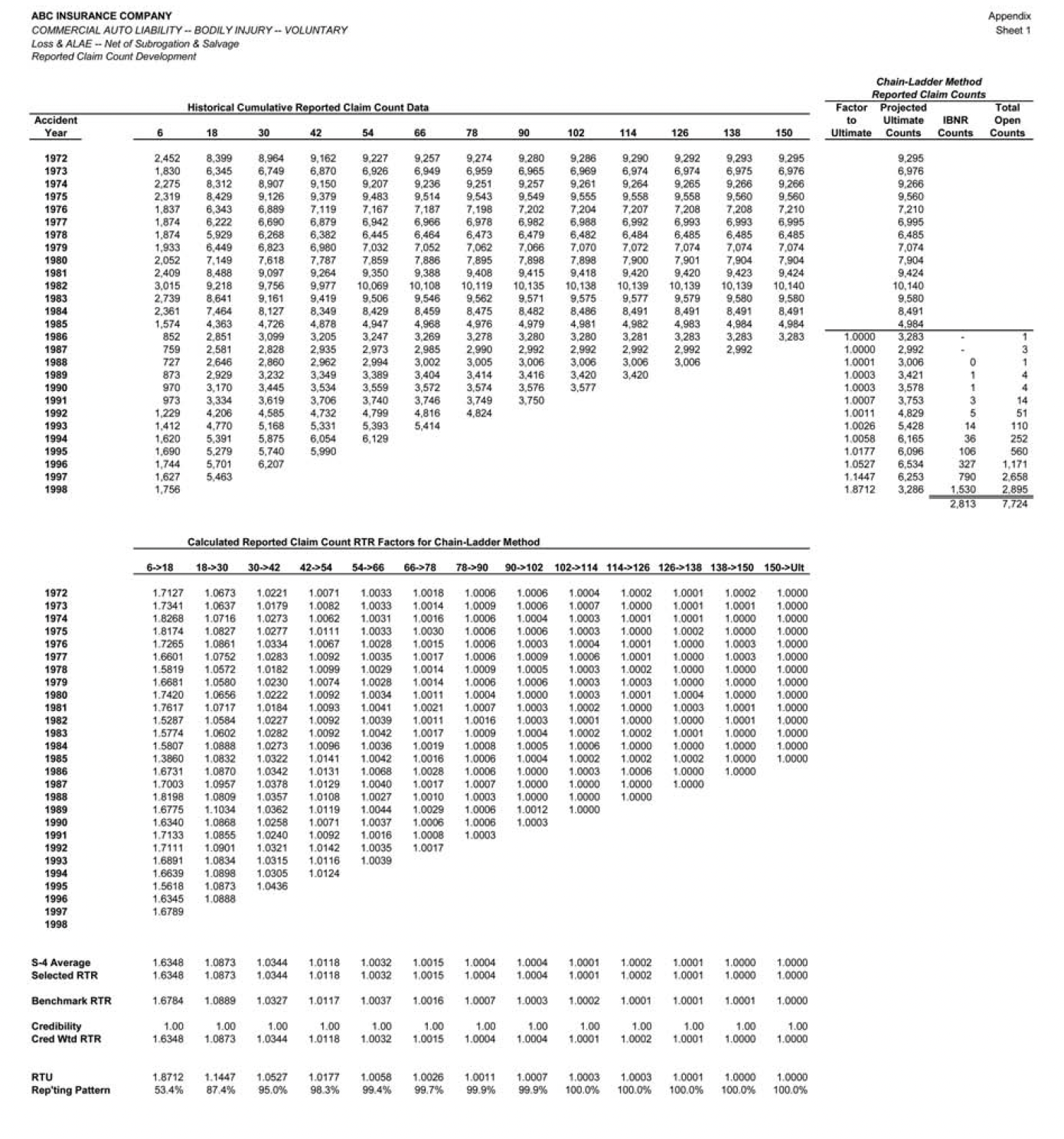
For each reserve segment, accident year loss development data is available for 27 accident years, from 1972 to 1998, with annual valuations at June 30. Sheet 1 of the Appendix illustrates the complete triangular dataset, displaying reported claim counts. This data facilitates claim liability estimation at each June 30 from 1979 to 1998, a 20-year span. During this same period, one of the authors provided independent estimates of claim liabilities to the management of the company, so actual historical projections using various methods are also available. Claim liability estimates at each of these 20 valuation points can be compared with “hindsight” estimates based on a special study performed using data through December 31, 2000, that combined actual run-off claim payments with estimates of the remaining unpaid claim liabilities at that time. Thus, for the most recent of the 20 estimates to be tested (i.e., the estimate at June 1998), the hindsight estimate reflects 30 months of actual run-off payments. For the earlier estimates, the hindsight estimate reflects an increasing proportion of actual run-off payments. Assuming that the December 2000 remaining claim liability estimates are a reasonable proxy for the actual remaining unpaid claim liabilities, the claim liabilities at June 1998 are 77% paid; the claim liabilities at June 1997 are 84% paid; the claim liabilities at June 1996 are 92% paid; and the claim liabilities at earlier valuations are between 96% and 100% paid.

For each reserve segment, loss development data consists of the following triangles:

• Reported claim counts (shown on Appendix sheet 1)

• Closed claim counts (combination of closed with payment and closed without payment)

• Paid loss and allocated loss adjustment expenses

• Incurred loss and allocated adjustment expenses (paid plus case reserves)

Fortunately, during this extended period the company’s claim systems did not change in material ways, so the historical data reflect relatively consistent claim processing, from an IT perspective.

In addition to the claim experience, direct earned premiums by calendar year are also available, allowing us to use methods based on loss ratios.

The company wrote what may be described as “main street business” through independent agents. The data is net of excess of loss reinsurance, at retentions that were relatively low, typically around $100,000.

The company’s historical experience provides a rich backdrop for illustrating performance testing, for several reasons.

• First, the experience period includes the '70s and early '80s, a period where significant monetary and social inflation caused trends and development patterns to change from their historical levels. Conversely, in the '90s this inflation abated and trends and development patterns stabilized.

• Second, the company made some significant operational changes—particularly to its claim handling procedures—that affected claim closure rates, case reserve adequacy, and the trends in average claim costs across accident years.

• Third, the company’s underwriting posture changed several times during the period. In the early experience years they focused on revenue growth, leading to relatively disastrous underwriting results (in this they were not alone). Eventually it became necessary to re-underwrite the existing business, become more selective about new business, and seek price adequacy.

These factors create some distinct “turning points” in the historical data, creating significant challenges to the claim liability estimation process. While the challenges in the future might take a different form than those observed in the past, the uncertainties created will potentially be of a similar magnitude. Thus we believe performance testing over this period is a useful exercise.

The case study focuses on our ability to estimate claim liabilities for Commercial Automobile Bodily Injury Liability (CABI). Estimation for this reserving segment is neither very difficult nor very easy, so it is a good place to start.

For the purposes of the case study we can pretend that it is 2001, and the company’s management has asked the corporate actuary to begin establishing a control cycle (making use of the “final” estimates of claim liabilities as of December 2000). The starting point is a performance testing project focusing on a representative line of business, CABI. The tests will include the two methods currently employed in the reserving process, the paid and incurred chain ladder methods; an alternative method, not currently used by the company, that projects case reserves only; and an additional incurred development method that seeks to adjust for changes in case reserve adequacy. While methods to adjust for case reserve adequacy have been in the literature for years, they have not been implemented at the company due to misgivings about their effectiveness and stability. The project is purposely limited in scope to fit within available resource constraints. As part of the project, a plan for further performance testing is also to be developed based on the initial results from the project.

4.2. Paid chain-ladder development method

The project starts with performance testing of the paid chain-ladder development (PCLD). First, we need to formally define the PCLD method, using our m(a,d,p) construct from the previous section. This is done in summary form in Table 2.

As can be seen in Table 2, this is a highly mechanical method, with little or no intervention, and no exogenous data employed. In essence, this is a test of “the machine,” without the normal dose of actuarial judgment supplied by “the man.” This is a scope limitation to the initial performance testing project; performance tests of the actuarial judgments are deferred to subsequent control cycles, after some experience with the performance of the basic methods has been gained.

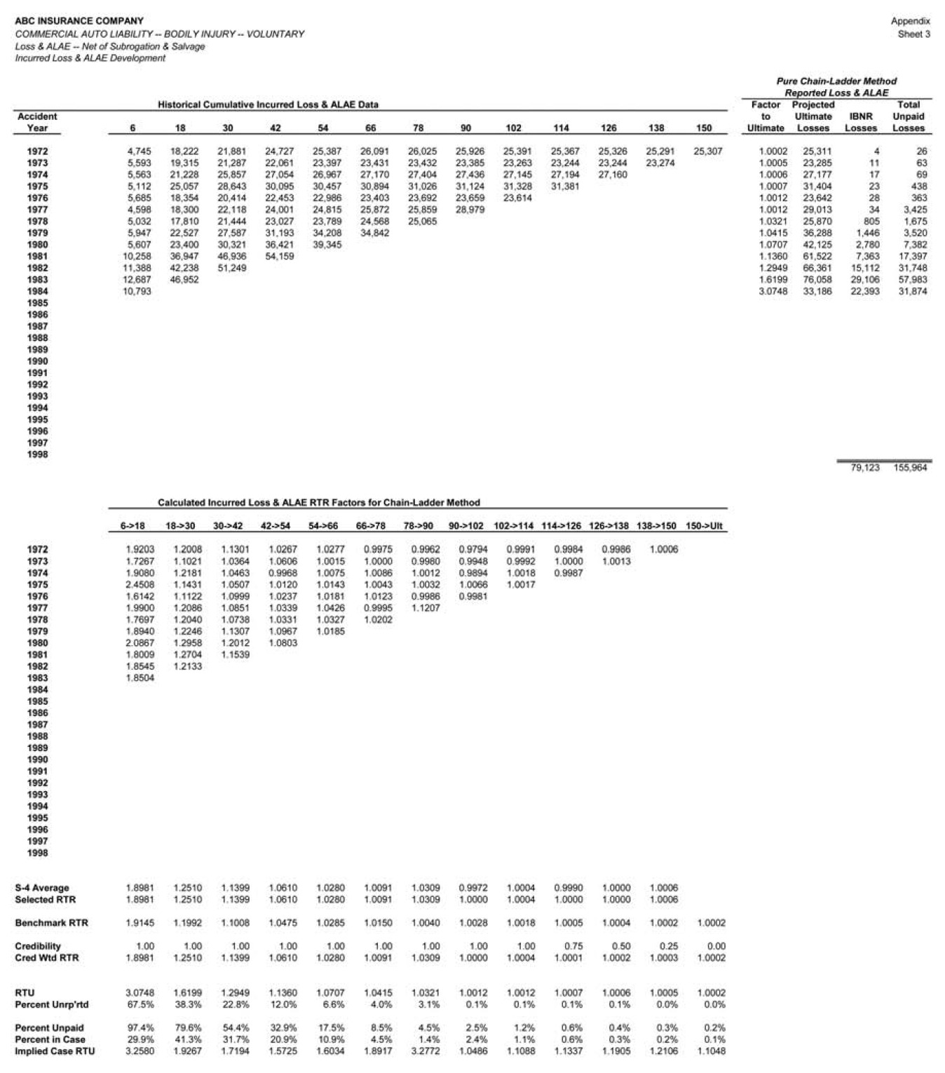
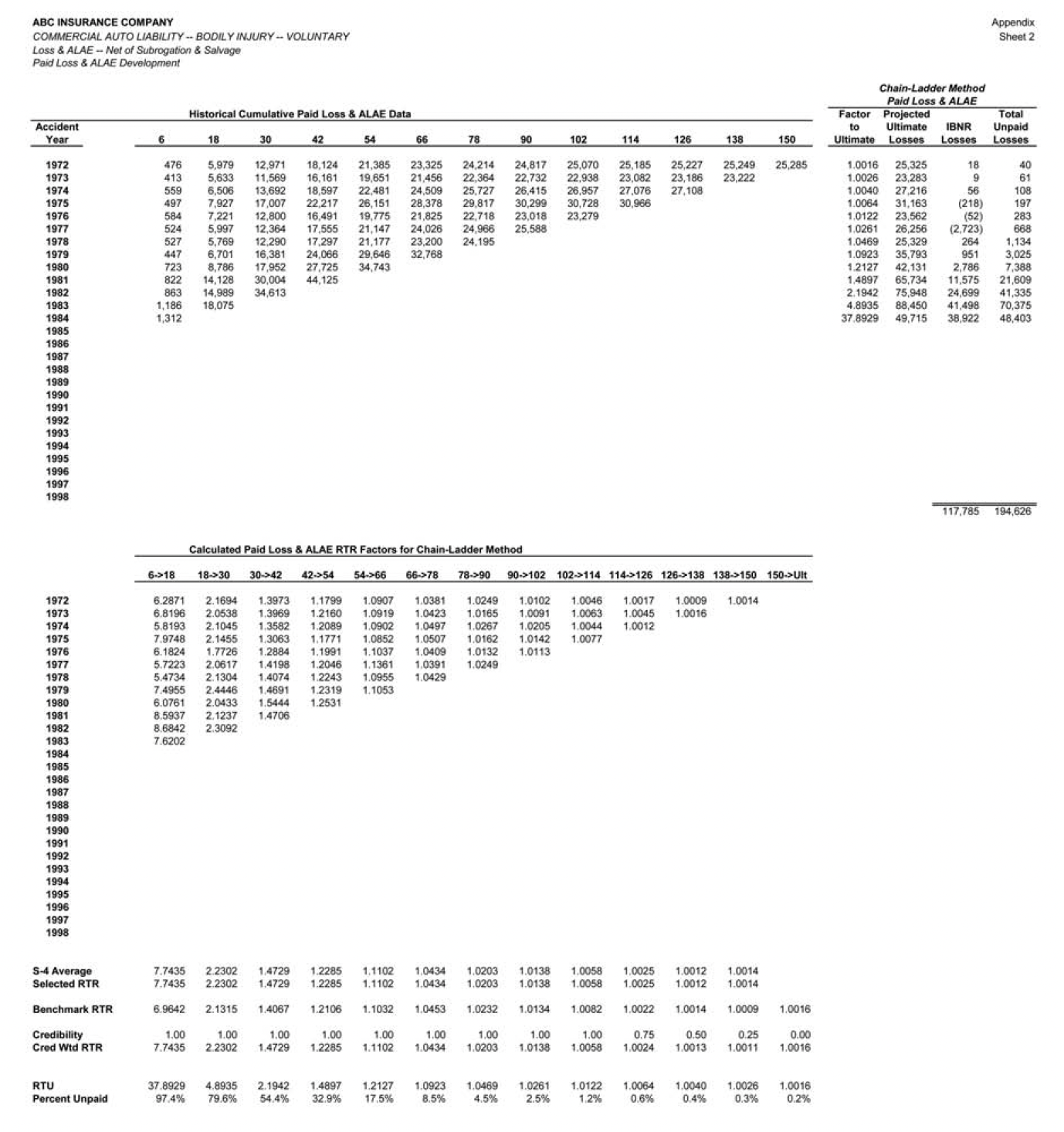
The PCLD method was applied to the available CABI data at each midyear valuation point from June 1979 to June 1998 to obtain estimates of the unpaid claims, by accident year, at each valuation. Application of the PCLD method at the June 1984 valuation is illustrated on sheet 2 of the Appendix.

Many actuaries find it convenient to vary actuarial projection methods by accident year, using one method for mature years, a different method for immature years, and perhaps yet another method for the current year. It will therefore be important to look at performance test results by maturity, to assist the actuary in his or her choices of method by maturity. Rather than focusing initially on the overall performance of the PCLD method, our analysis therefore starts with a single component of the claim liability, the performance results for the accident year at 42 months maturity. (The choice of 42 months is arbitrary.)

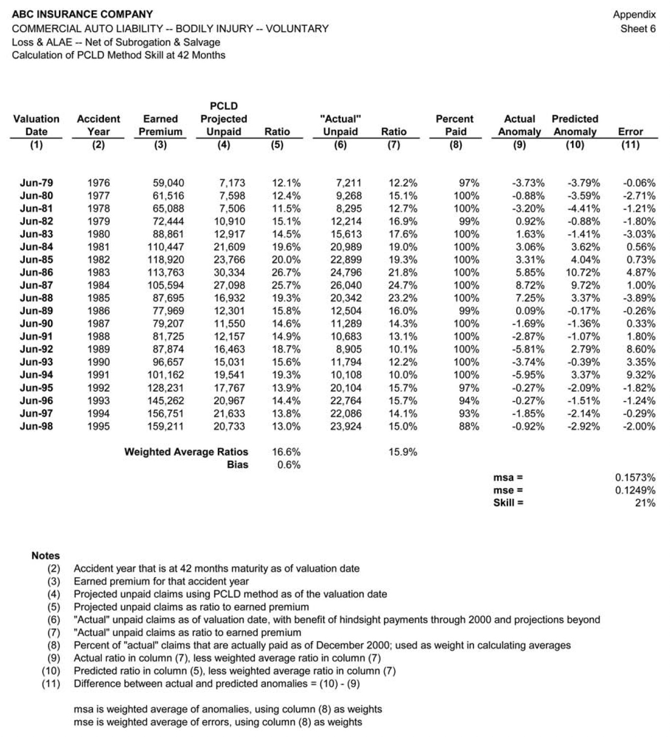
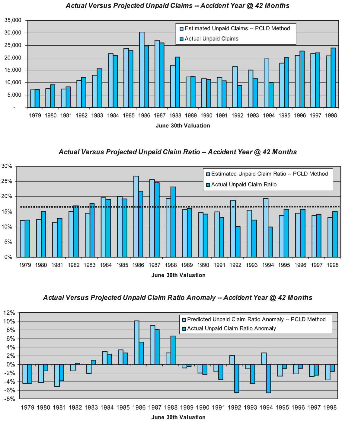
Figure 3 displays the performance of the PCLD method as an estimator of the unpaid claims for the accident year at 42 months maturity (i.e., the 1976 accident year at the June 1979 valuation, the 1977 accident year at the June 1980 valuation, etc.) The results in Figure 3 are designed to answer the question “How accurate is the paid chain-ladder development method as an estimator of unpaid claim liabilities when applied to the actual cumulative paid claims at 42 months maturity?”

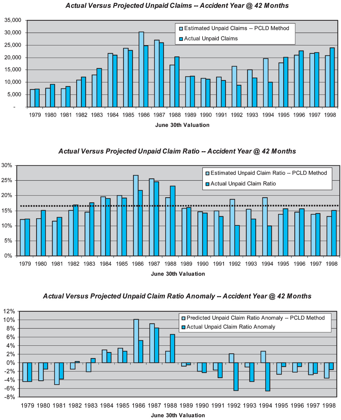
The uppermost of the three bar graphs in Figure 3 compares the estimated unpaid claim liabilities to the actual unpaid claim liabilities at each valuation point. (Note that, by “actual,” we mean the unpaid claims with the benefit of hindsight through December 2000, consisting of actual payments through December 2000 plus estimated unpaid claims at that point.) One can see that there is some degree of correspondence between the PCLD estimate and the actual liabilities, although at some valuations (1986 and 1992–1994) the correspondence is not terribly strong.

The middle of the three bar graphs converts the predicted dollars of unpaid claim liabilities into unpaid claim ratios, by dividing them by the earned premium for the calendar year. This essentially normalizes for variations in the volume of business. The dotted horizontal line is the average unpaid claim ratio, which is approximately 16%. (Note that the premium being used is the combined liability premium for both bodily injury and property damage; these are only the bodily injury portion of the loss ratio.) The overall picture isn’t materially different than the upper bar graph, partially because the company had the misfortune to maximize its volume of business in the late '80s, when loss ratios were highest. The relative heights of the pairs of bars are largely unchanged.

Finally, the lowermost bar graph of Figure 3 simply adjusts the unpaid claim ratios by subtracting the 17% average unpaid claim ratio. The result is to express the projections in terms of their ability to detect deviations from the average. This last presentation is relevant because the skill of a forecasting method is typically defined as

$$\text { Skill }_{m}=1-m s e_{m} / m s a \tag{4.1}$$

where mse_m is the mean squared error, the average squared difference between the actual unpaid claim ratio and the predicted unpaid claim ratio from the method; and msa is the mean squared anomaly, the average squared difference between the actual unpaid claim ratio for that observation and the overall average actual unpaid claim ratio across the entire test period. The mse_m is specific to the actuarial method, while the msa is an intrinsic property of the experience. The method with the minimum mean squared error will therefore have the maximum skill.

Does the form of the measure of skill look familiar? In a regression context it would be expressed as

$$R^{2}=1-s s e / s s t \tag{4.2}$$

where sse is the squared difference between the actual values and those predicted by the regression equation, and sst is the squared difference between the actual values and their mean. Just as R² is a statistical measure of amount of variation captured by the regression equation, Skill_m is a measure of the amount of variation captured by the particular actuarial method.

Those familiar with credibility will also recognize that there is some similarity of the definition of skill to that of credibility.

From the definition of skill, one can recognize that skill is equal to zero when the mse_m is equal to the msa, and negative when the mse_m is greater. In these cases one would be better off multiplying the earned premium by the long-term average unpaid claim ratio to estimate the unpaid claim liabilities, rather than using the method being tested.^[8] Conversely, when the mse_m is zero, the method perfectly predicts the actual result and skill is 100%.

Returning to the lowermost bar graph on Figure 3, one can observe the actual unpaid claim ratio anomalies directly. They reflect the pattern of the underwriting cycle during this era. The actual unpaid claim ratio anomaly is contrasted with the predicted anomaly. The errors are the differences between the pairs of bars, reflecting our ability to predict the direction and magnitude of the anomaly. While it is not a fundamental transformation, removing the mean improves the visual display, allowing one to see the errors more clearly. This lower chart is the typical means of displaying performance test results.

The skill of the paid chain-ladder method in estimating the unpaid claims at 42 months for an accident year is only about 21%. This result is heavily driven by the poor performance of the method at the June 1986, 1992, 1993, and 1994 valuations. At each of these valuations, the PCLD projections look reasonable based on the information available at the time; however, subsequent paid claim development is markedly different than the history up to that point.

The data underlying Figure 3, along with the details of the calculated skill of 21%, are presented on sheet 6 of the Appendix.

Skill can be measured at other maturities, using the same approach as is depicted in Figure 3. It turns out that the PCLD method does not exhibit much skill in this case. Skill is actually at its highest, at 21%, at 42 months maturity. The skill of the PCLD method in estimating an accident year’s unpaid claims at both earlier and later maturities is actually negative. For the early maturities, the size of the development factors becomes so large that the estimates become very volatile. For the very mature years the remaining unpaid claim liabilities are small and highly dependent on the numbers and nature of the claims that remain to be settled, so the volume of cumulative paid claims is just not a very good indicator of the remaining unpaid claims. Many readers will recognize these as being typical shortcomings of the PCLD method.

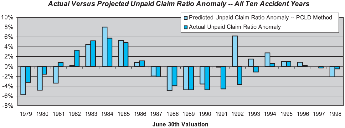
It is easy to extend the skill measure to the overall estimate of unpaid claims across all accident years, by merely taking the weighted average of the individual accident year unpaid claim ratios. Rather than using all accident years, we have elected to use only the latest 10 accident years, so that the metric is relatively consistent over time. The results are shown on Figure 4.

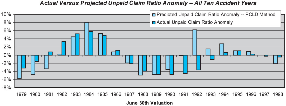
Our performance test results indicate that the overall skill of the paid development method in estimating unpaid claim liabilities for all 10 accident years combined is only about 13%. The low skill is driven by the large prediction errors at the 1981, 1991, and 1992 valuations. At each of these valuations the PCLD projections look very reasonable; however, the subsequent development looks markedly different than the history up to that point.

The PCLD method also exhibits some shortcomings against our other BLURS-ICE criteria. Over the 20-year performance test period, the method exhibited a positive bias (predicted dollars of claim liabilities above actual liabilities) of about 4%. Given the volatility of the prediction errors, this is likely to simply reflect sampling error. The method is also unresponsive to changing conditions; not surprisingly, it tends to react in a lagged manner to changes in the payment pattern.

One reason for the low skill of the PCLD method in this particular case is the nonstationarity of the claim settlement process over the historical period, as evidenced by the changing percentages of claims open in Figure 5. This figure suggests that an adjusted paid method, reflecting the changing claim settlement rates, should offer improved skill over the simple method we have employed here.

Overall the PCLD performance tests suggest that this method is of little value, with very low skill, due to the changing patterns of claim settlements. The skill of the PCLD on this product line would be higher in more normal circumstances, when settlement patterns are more stable. Performance tests of methods that adjust for changes in settlement patterns could be undertaken. At a minimum, simple diagnostics that detect changing settlement patterns should be introduced into the reserving process so that the actuary can know when the PCLD is not likely to produce a reasonable estimate.

4.3. Incurred chain-ladder development method

We turn next to performance testing of the chain-ladder method applied to incurred (paid plus case reserves) claim development data (ICLD). Once again we start by formally defining the method, as summarized in Table 3.

As was the case with the paid method, our approach is insular and largely mechanical, without benefit of judgment or confirming tests based on exogenous data.

We applied the ICLD method to the CABI incurred development data at each midyear valuation point from June 1979 to June 1998 to obtain estimates of unpaid claims at each valuation point. (More specifically, we used the ICLD method to estimate the Incurred But Not Reported [IBNR] liabilities, and then added the case reserves to get total estimated unpaid liabilities.)

Application of the ICLD method at the June 1984 valuation is illustrated on sheet 3 of the Appendix.

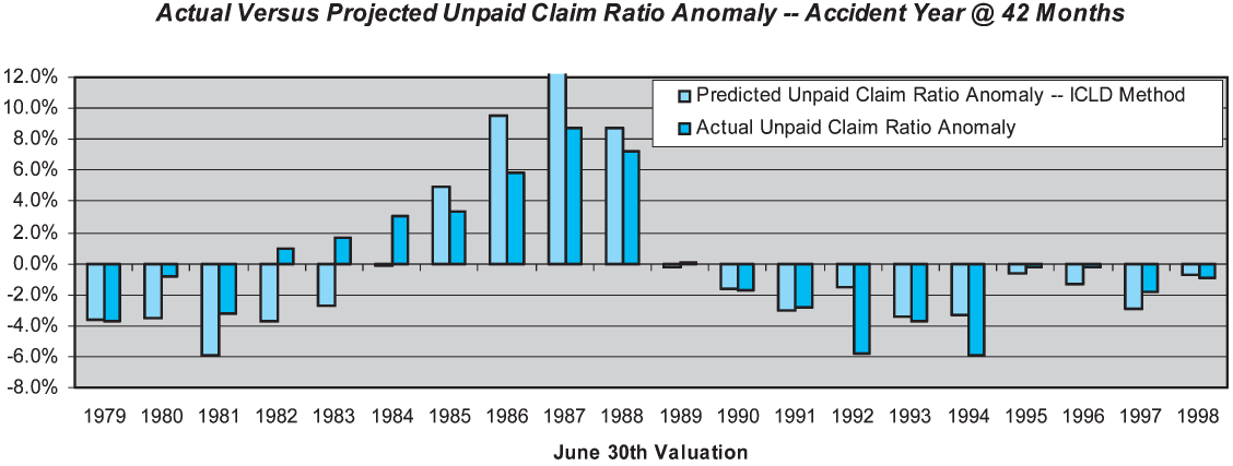
The ICLD performance test results for the accident year at 42 months are shown in graphical form in Figure 6. This graphic is analogous to the lower graphic in Figure 3, comparing predicted unpaid claim ratios to actual unpaid claim ratios with the benefit of hindsight.

As can be seen in Figure 6, the ICLD method performs poorly in the 1981–1984 period, underestimating the unpaid loss ratio. It then performs poorly in the 1986–1987 period, overestimating the unpaid loss ratio. In 1992–1994 it again overestimates the unpaid loss ratio.

The ICLD method exhibits better skill than the PCLD method, but its absolute skill is still relatively low. The observed skill of the ICLD method at 42 months maturity is 52%, versus 23% for the PCLD method. The skill of the ICLD method is negative for the most recent (18 months) maturity and for the older maturities.

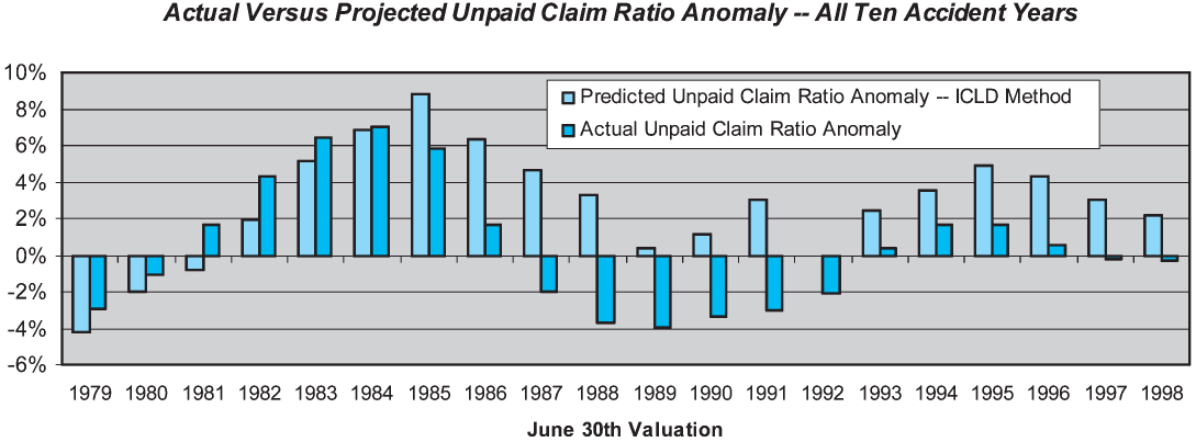
Overall the skill of the ICLD method for the last 10 accident years combined is 31%, versus 13% for the paid chain-ladder development method. Figure 7 displays the overall performance test results for the ICLD method.

Over the 20-year performance test period the ICLD method exhibited a negative bias (predicted dollars of claim liabilities below actual liabilities) of 0.8%. However, this is not likely to be a statistically significant result.

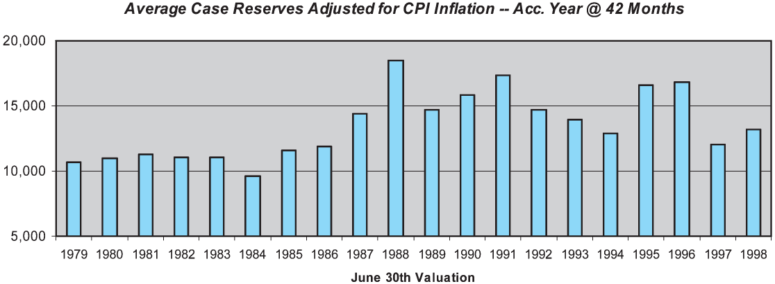
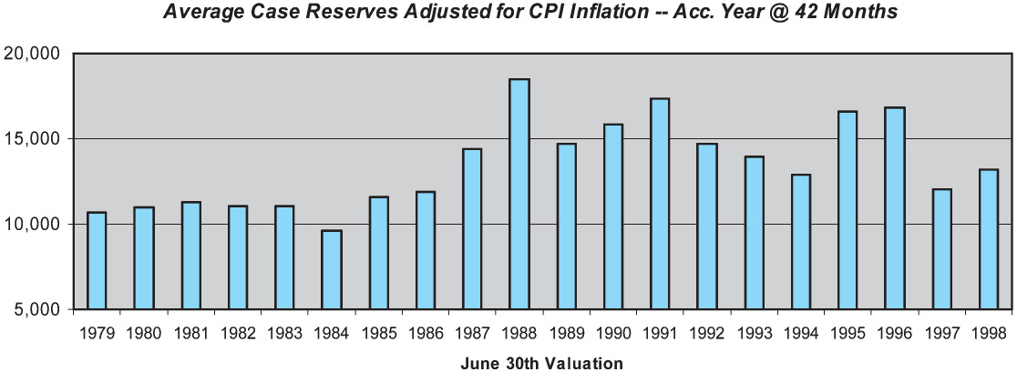
One reason for the poor skill of the ICLD method is the changing levels of case reserve adequacy over the historical period, due to the changes in claim handling procedures mentioned earlier. Figure 8 displays the average case reserve on open claims for the accident year at 42 months, adjusted to a constant-dollar basis using the U.S. Consumer Price Index (CPI). As can be seen, the average case reserve for the accident year at 42 months increased substantially during the period from 1984 to 1988. While somewhat volatile, the average case reserve also appears to have declined from its 1988 peak level during the early 1990s. This suggests that an adjusted incurred method, reflecting changes in case reserve adequacy, would offer improved skill over the simple incurred chain ladder method. We test such a method later in this section.

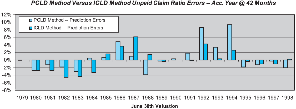
One can compare the PCLD and ICLD methods directly by looking at their prediction errors, as is shown in Figure 9. Inspection of the errors shows that the root cause of the performance difference between the PCLD and the ICLD is the performance of the former in the years 1992 and 1994. These two years contribute significantly to the mean squared error of the paid chain-ladder method. Prior to this period, the company engaged in a significant effort to reduce the inventory of open claims. This manifested itself as higher-than-average paid development, which translated into several diagonals of above-average paid development factors. As these factors worked their way through the average, the paid chain-ladder forecasts significantly overshot the mark.

Looking at the errors more broadly, one can see that they are similar during some periods and only occasionally divergent.

Before continuing with performance tests of other methods, we diverge to look at the issue of combining estimates from multiple methods.

4.4. Combining estimates from multiple methods

We now have predictions from two actuarial projection methods, PCLD and ICLD, with measures of skill for each. The next question to be addressed is how to combine the results of the two methods together to create a single actuarial central estimate. We want to combine the two estimates according to

$$\hat{L}_{C}^{(t)}=w \times \hat{L}_{I}^{(t)}+(1-w) \times \hat{L}_{P}^{(t)} . \tag{4.3}$$

We want to choose w so that the variance of the error distribution around $\hat{L}^{(t)}_{C}$ is minimized. The variance of the error distribution around $\hat{L}^{(t)}_{C}$ is given by

$$\begin{aligned} V_{C}= & w^{2} \times V_{I}+2 \times w \times(1-w) \\ & \times \operatorname{Cov}\left(\hat{L}_{I}^{(t)}, \hat{L}_{P}^{(t)}\right)+(1-w)^{2} \times V_{P} \\ = & w^{2} \times V_{I}+2 \times w \times(1-w) \times \rho_{I, P} \\ & \times \sigma_{I} \times \sigma_{P}+(1-w)^{2} \times V_{P} \end{aligned} \tag{4.4}$$

where V_I, V_P, V_C are the variances of the estimation errors for $\hat{L}^{(t)}_{I}$, $\hat{L}^{(t)}_{P}$, $\hat{L}^{(t)}_{C}$, respectively, σ_I,σ_P are the standard deviations of the estimation errors for $\hat{L}^{(t)}_{I}$, $\hat{L}^{(t)}_{P}$, respectively, and $\rho_{I, P}$ is the correlation coefficient between $\hat{L}^{(t)}_{I}$, $\hat{L}^{(t)}_{P}$.

To minimize the error distribution around $\hat{L}^{(t)}_{C}$ we must merely take the derivative of V_C with respect to w, set the derivative equal to zero, and solve for w. Doing so we get

$$w=\frac{V_{P}-\rho_{I, P} \times \sigma_{I} \times \sigma_{P}}{V_{I}-2 \times \rho_{I, P} \times \sigma_{I} \times \sigma_{P}+V_{P}} \tag{4.5}$$

One can see from Equation 4.5 that if the variances of the error terms are equal, then w is equal to 50%. If the variances of the error terms are not equal, greater weight will be given to the method with the lower error variance, depending on the correlation.

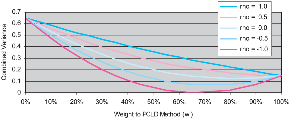
Figure 10 provides additional insight to the relationship between the two variances and the correlation. In this example, V_P = .65 and V_I = .15. The chart shows how V_C varies with w for a given level of correlation (“rho” in the chart), with the minimum combined error variance being the lowest point on each curve. If there is perfect positive correlation between the estimation errors $\left(\rho_{I, P}=1.0\right)$, then the combined error variance is minimized by simply giving 100% weight to the method with the lower error variance. As correlation decreases, one can see that the minimum combined error variance entails giving some small weight to the method with the higher error variance. At the extreme, if the estimation errors for the two methods are negatively correlated, then they can be perfectly offset to produce zero combined error variance by using weights from Equation 4.5—in this case approximately a 67.6% weighting to the lower variance estimate.

In the specific case of our CABI results for the accident year at 42 months, we have the following.

• The mse of the PCLD method is 0.1249%.

• The mse of the ICLD method is 0.0753%.

• The observed correlation between the errors of the two methods is 60.3%.

Assuming that these were the only two methods available and we believed that the historical performance test results were reasonable indicators of the current situation, then the indicated minimum-variance weighting would be 79.5% to the estimate from the ICLD method with the balance given to the estimate from the PCLD method. The mse of the weighted average is 0.0719%, an improvement over either of the standalone methods.

The weighting approach derived in this section could obviously be applied by individual accident year with varying weights, or to the overall estimates from each of the methods using weights based on the variances and correlations between the overall errors of the methods. It is easily extendable to more than two methods, by expansion of the combined variance equation to:

$$\begin{aligned} V_{c}= & \sum_{i=1}^{n} w_{i}^{2} \times V_{i}+2 \times \sum_{i=1}^{n} \sum_{j=1, j>i}^{n} w_{i} \\ & \times w_{j} \times \rho_{i, j} \times \sigma_{i} \times \sigma_{j} \end{aligned} \tag{4.6}$$

Again, to minimize the combined variance one must take the derivative of V_C with respect to w_i, subject to the constraint that $\sum_{i=1}^n w_i=1$.

As the number of actuarial projection methods gets larger, the required number of estimates certainly grows, including the estimates of the variance of each method and the correlation coefficient between each pair of methods.

4.5. Case reserve development method

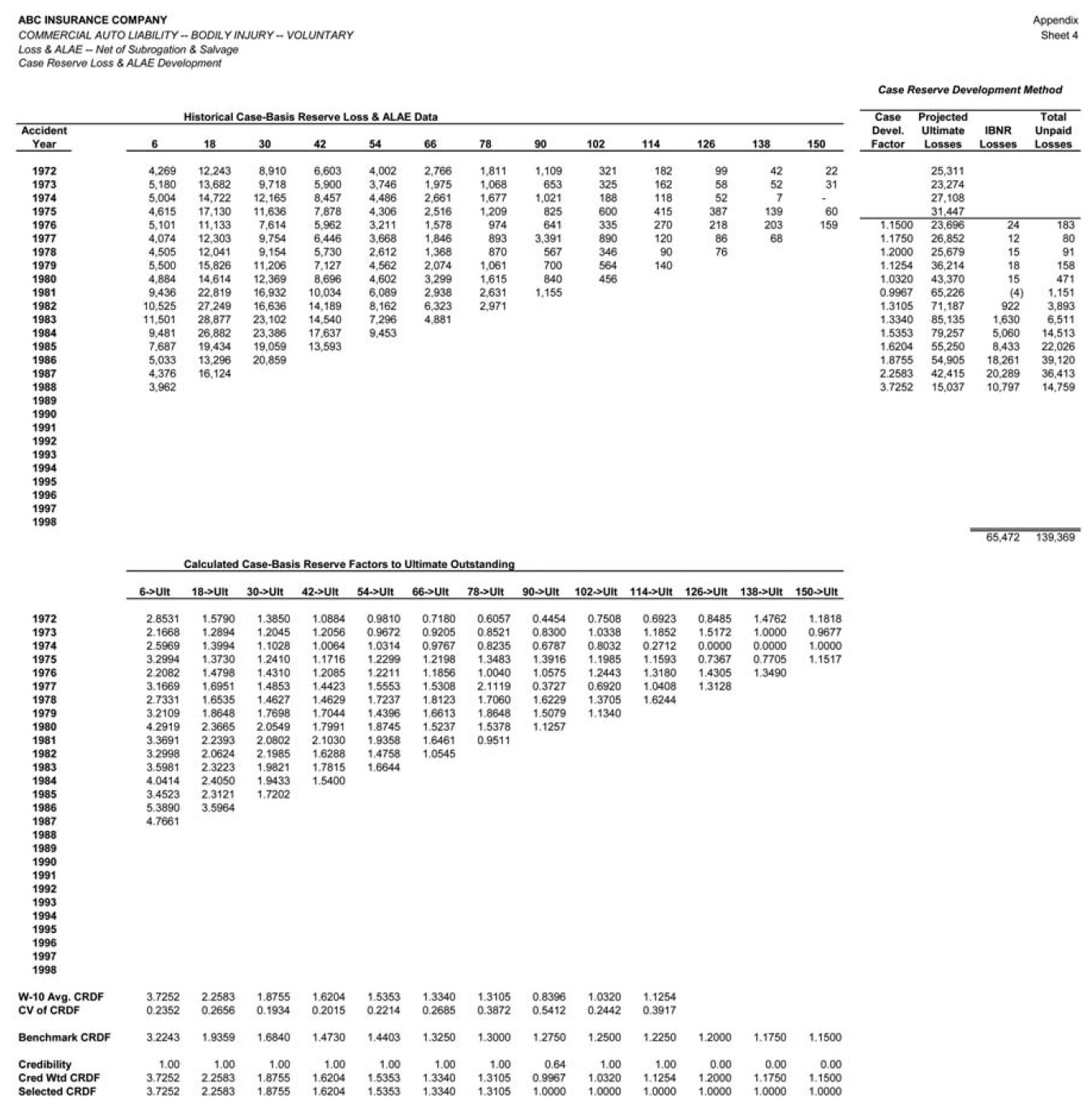
The next actuarial projection method we tested was the case reserve development method (CRD), in which a development factor is applied to the unpaid case-basis claim reserves for each accident year to obtain the estimated unpaid claim liability. The CRD method is a recursive approach, in that the projections from earlier accident years are used to calculate the factor to be applied to the next accident year, successively. The CRD method is formally defined in Table 4.

Application of the CRD method at the June 1988 valuation is illustrated on sheet 4 of the Appendix.

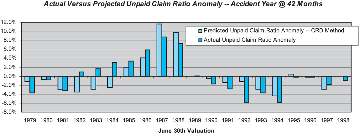
Performance test results for the CRD method for the accident year at 42 months maturity are shown in Figure 11.

The CRD method exhibits better skill than either the paid or incurred development method at older maturities. The observed skill of the CRD method at 42 months is 58%, versus 52% and 23% for the ICLD and PCLD methods, respectively. The observed skill of the CRD method at 54 months is even higher, at 67%. Similar results have been obtained by the authors in performance test results for other liability lines. It appears that for mature years, in liability lines the case reserves alone are a better predictor than the incurred (i.e., paid plus case reserves) claims. This makes some intuitive sense, as the case reserves relate directly to future claim payments on open claims, whereas the cumulative paid claims relate to claims that are closed which are unrelated to future claim payments. The skill difference is particularly notable when the remaining case reserves are variable, significant in some accident years and less significant in others.

The overall skill of the CRD method across the latest 10 accident years is 22%, substantially lower than the 32% skill of the ICLD method, primarily because the CRD method has very little skill for the early maturities.

4.6. Reported claim count chain-ladder development

Since projecting claim counts does not (by itself) yield an estimate of unpaid claim liabilities, it does not technically qualify as an actuarial projection method. Nonetheless, we tested the performance of the chain-ladder applied to reported claim counts (RCCLD). Once again we use a highly mechanical method, as outlined in Table 5 and illustrated at the June 1998 valuation on sheet 1 of the Appendix.

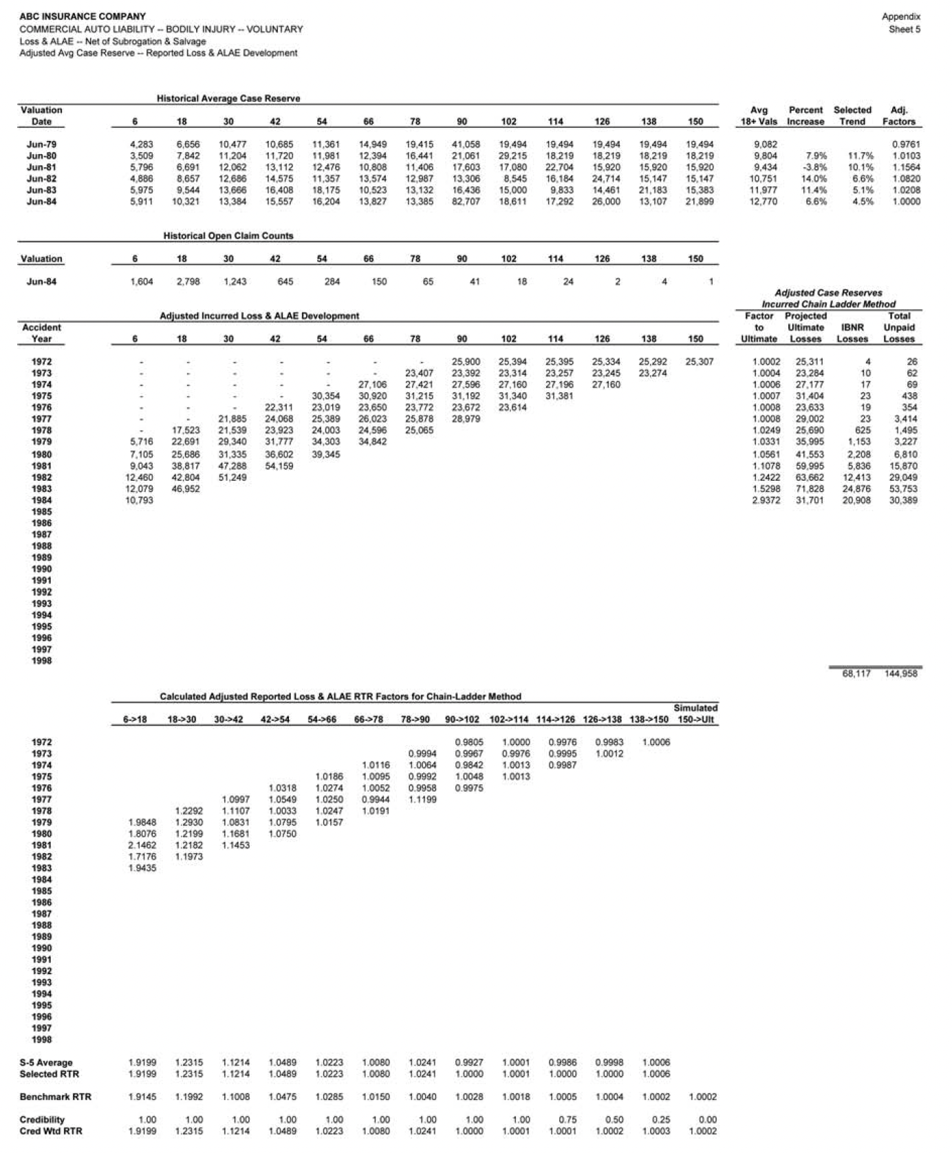
Application of the RCCLD method is illustrated for the June 1984 valuation on sheet 5 of the Appendix.

Figure 12 displays the performance test results for the RCCLD method for the accident year at 42 months. The RCCLD method exhibits remarkably better skill than any of the other methods tested, primarily due to the stability in the claim reporting process over the study period. Measured skill at 42 months is 99%. While case reserving policy and settlement practices changed dramatically, the reporting of claims into the claim system did not.

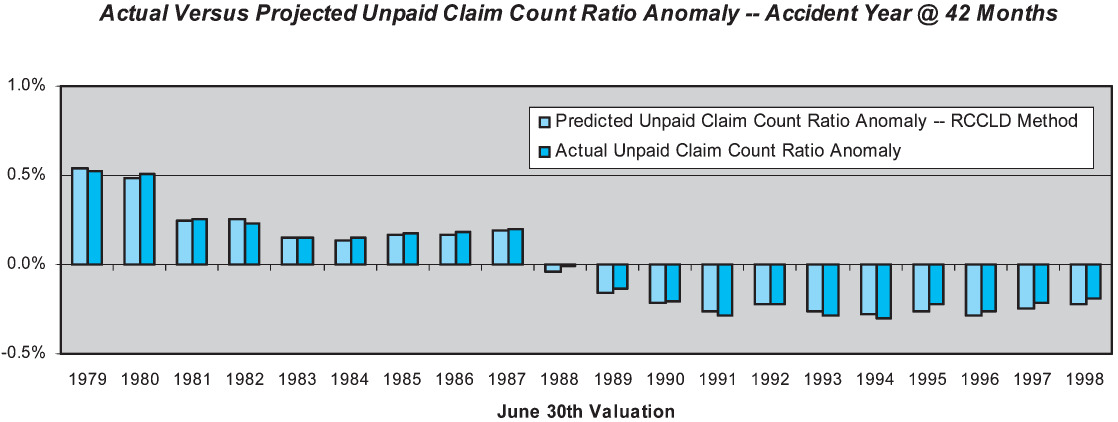
The skill of the RCCLD method is high at all maturities, ranging from a low of 95% at six months to a high of 99% at 42 months and beyond.

The clear implication is that the claim count data has very high information value. Methods that make use of the count data should therefore have enhanced predictive skill over methods that use only the dollar data.

4.7. Incurred chain-ladder with case reserve adequacy adjustment

As was noted earlier, the historical experience exhibits significant changes in case reserve adequacy at various points in time, reflecting changes in case reserving policies at the company. We therefore have tested the performance of a method that measures and adjusts for case reserve adequacy before applying the incurred chain-ladder method. We will refer to the method as case-adequacy adjusted incurred chain-ladder development (CAAICLD). The method is summarized in Table 6, and illustrated at the June 1984 valuation on sheet 5 of the Appendix.

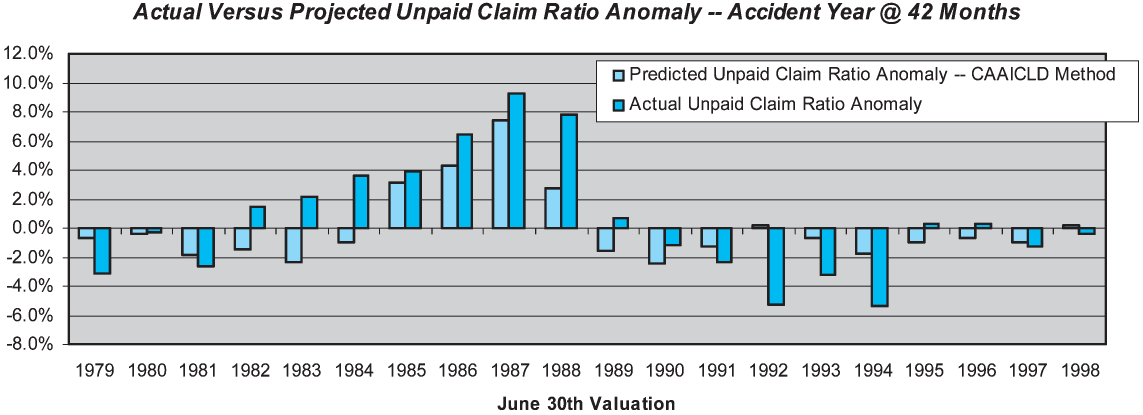
For comparison purposes, we start by analyzing the performance results for the accident year valued at 42 months maturity. Results are displayed in Figure 13.

The skill of the CAAICLD method at 42 months maturity is 52%, exactly the same as the unadjusted ICLD method. However, a comparison of Figure 13 with Figure 6 shows that the estimation errors occur at different points in time. The correlation of the estimation errors is only 37%. At this maturity, the CAAICLD method reduces the estimation errors caused by the changes in case reserve adequacy, but introduces new errors due to the imperfections of the case adequacy adjustment process.

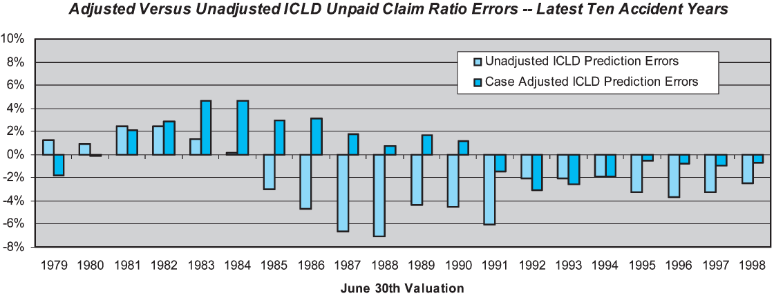
However, the overall skill of the CAAICLD across the latest 10 accident years is substantially higher than the unadjusted ICLD method, 52% versus 31%. While skill is not enhanced at 42 months, it is substantially enhanced at 18 and 30 months. The reasons for the overall skill enhancement can be seen in Figure 14. The overall magnitude of the estimation errors is reduced by the case adequacy adjustment. Whereas the unadjusted method produced estimation errors greater than six loss ratio points three times, the adjusted method never produces errors of that magnitude. The adjusted method is far from perfect, as it produces errors in excess of four loss ratio points twice in the test period. The results might be further improved by the use of an inflation index that was more relevant to CABI claim costs, or by other alternative adjustment techniques than those we employed.

4.8. Summary conclusions from the case study

The case study presented in this section only begins to scratch the surface of performance testing. Test results for many additional methods, and variations on each one, could have been presented—making for a very long paper indeed.

In addition, it is hard to present the test results in a paper format, as much of the real insight comes from poring over the details of the calculations. Our goal was merely to illustrate the methodology and demonstrate the potential insights that can be gained from it, making the case for incorporating it into an ongoing control cycle for the reserving process. The key takeaways we would highlight from the case study are the following:

• The accuracy, or skill, of actuarial methods can be formally tested using the cross-validation approach employed in other predictive sciences. Formal performance testing can help the actuary to understand the strengths and weaknesses of each method, and more realistically assess the potential estimation errors arising from them.

• Performance testing can guide the actuary in the selection of methods, both overall and by maturity. It also provides a methodology for combining the estimates produced by different methods. Correlation between the methods is relevant to the selection of methods, and the weighting scheme used to combine them.

• The accuracy of the basic chain-ladder methods is seriously degraded when there are changes in underlying claim policies and processes. The level of skill indicated by the case study is lower than one would expect absent these changes. These changes are often detectable by analysis of claim settlement rates or average case reserves, which require claim count data. Adjusting for changes in underlying claim policies and processes enhances skill.

• Claim count development is often more predictable than claim dollar development, especially when there are changes in claim procedures and processes. In these situations, methods that make use of the claim count data are likely to improve the accuracy of the estimates.

• Experimentation with less traditional methods may lead to enhancements in skill. Our experimentation with the case reserve development method (including tests not covered in this paper) suggests that it does outperform incurred chain-ladder in many liability lines.

Areas for further exploration would obviously include testing of methods that adjust for changes in claim settlement rates as well as changes in case reserve adequacy. In addition, tests of more complex methods, including regression-based and stochastic methods, would be of interest.

Finally, it would be useful to test whether overall skill is higher when the Bodily Injury Liability claims are combined with the Property Damage Liability claims into a single projection, versus separate projections on each. While homogeneity of the claims is a desirable property—arguing for greater granularity—one of the authors believes that greater consolidation often leads to greater credibility (i.e., reduced noise in the data) and improved skill. Further performance testing will help to find the optimal trade-off between improved homogeneity and improved credibility.