Yep, We’re Skewed

All of us, especially those of us working in insurance, are constantly exposed to the results of small samples from skewed distributions. The majority of our customers will see small sample results below the population mean. Also, the most likely sample average value for any small sample from a skewed population will be below the mean of the skewed population being sampled. Experienced actuaries are aware of these issues. However, we have to be on guard and not fall back on easy assumptions that are appropriate for results from symmetrical distributions.

For a symmetrical distribution with one mode, such as a bell curve, the mode is equal to the mean. But for a typical distribution that we might encounter in insurance that is skewed to the right and that has only one mode, the mode is less than the median, which is less than the mean. When we do small samples from typical skewed distributions, the most likely value for the sample average of a small sample will be somewhere between the mode and the mean of the sampled distribution. How close our small sample average will be to the mode or to the mean of the sampled distribution will depend on the sample size and the skewness of the distribution from which we are sampling. Moreover, for some skewed distributions, “small” samples can be surprisingly big.

For some insurance examples, this relationship should be in the back of our minds. Take, for example, the annual sample from a highly skewed distribution such as the annual hurricane losses in the city of Miami. For any particular year, the most likely loss we will observe is zero—the mode of the distribution. Every so often there will be a hurricane loss that will bring the long-term average above the zero mark, but most of the time we will see no losses.

On the other hand, an industry average loss ratio is based on a sample size that we could consider for all practical purposes to be infinite. If we are dealing with large samples, even from skewed distributions, we are confident that the most likely value for the sample average will be something close to the true average of the distribution.

In between these two extreme cases—a sample size of one and a sample size that is virtually infinite—the most likely value for the average of the sample goes from the mode of the sampled distribution up to the mean of the sampled distribution. As an example, let us examine the results from a positively skewed distribution used in insurance modeling—the lognormal distribution.

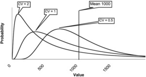
Figure 1 shows three lognormal curves, each with a mean of 1,000 and with varying degrees of skewness. As the skewness increases, the mode or highest point on the distribution is associated with points closer and closer to zero.^[1] For a log-normal distribution with a coefficient of variation (CV) of 2.0, the most likely value for a sample size of one is relatively close to zero, no matter how big the mean of the distribution. For small samples from this skewed distribution, the most likely value for the sample average will be close to zero.

Figure 1.Lognormals with mean 1,000.

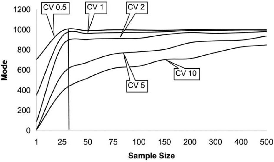
In order to give a feel for what makes up a small sample size, I simulated random values from a lognormal distribution with a mean 1,000 and varying degrees of skewness. The modes for the sample averages of various sizes are shown in Figure 2 for lognormal distributions with a mean of 1,000 and CVs of 0.5, 1.0, 2.0, 5.0, and 10.0.

Figure 2.Mode of sample average.

For individual claim size distributions that have low skewness, the most likely value that we will see from a sample average very quickly approaches the mean of the distribution. Many introductory statistical textbooks give a rule of thumb that infinity begins at a sample size of 30, and for low skewness 30 does seem to be a magic number when we are dealing with the log-normal distribution. However, as the skewness increases, it takes a very big sample size before the most likely value of the sample average approaches the mean of the sampled claim distribution. For a lognormal distribution with a CV of 10, even at a sample size of 500, the most likely value we would see from the sample average is 85% of the distribution mean. Formal credibility formulas aside, I believe many actuaries would consider 500 homogeneous claims to be a fairly large database.

With a CV of 10 and a sample size of 10,000, the most likely value we would see is still only 96% of the mean of the distribution. A simulation size of 10,000 is not an uncommon size for actuaries doing simulations. Even with this large sample, there is still a downward bias of 4% from the actual average of the distribution.

Another thing to observe about these sample results is that the most likely values for the sample averages follow a pattern of rising quickly from the mode of the distribution and then hitting a fairly flat area that approaches the mean very slowly. In his book Fooled by Randomness (2001), Nassim Taleb discusses how people are misled by skewed distributions. He focuses on the rare extreme values in the tail of the distribution, which he calls the black swans that are usually missing from the sample results out of skewed distributions. People forget about these black swans or are unaware of them.

However, for “small” samples out of skewed distributions, it is not just missing black swans that can cause problems. We may be getting ugly ducklings in our small samples. The most likely values of small samples from skewed distributions are actively misleading the observer because the mode of the sample average is so much lower than the mean. It is almost as if the skewed distribution is actively evil by feeding us misleading information from its body as opposed to passively withholding tail information from us. If we say that risk is a function of the standard deviation, then the presence or absence of black swans would have a greater impact on our perception of the risk of a loss process than on the mean of the loss process.

When we are doing relatively small samples from skewed distributions, we should recognize that the most likely value of the sample average will be less than the mean of the distribution that we are trying to measure. We should also realize that the sample of points we are working with is composed of even smaller samples that our individual customers see. The majority of our customers will see results lower than the long-term average and perceive the average we calculate as too high. Actuaries can try to deal with issues associated with small sample sizes with techniques such as maximum likelihood estimates to solve for distribution parameters, analyzing the data by splitting it into basic and excess limits, or using catastrophe models. However, we are still faced with the problem of customer perceptions as a result of skewed distributions, and perception is reality. Yep, we’re skewed.

Along these lines, Ted Kelly, CEO of Liberty Mutual (Friedman 2006) warned about pricing levels in the 2006 property market. Property insurance prices had increased dramatically because of the losses associated with Hurricane Katrina in 2005 and presumably due to the early predictions by the hurricane forecasters of severe hurricanes for 2006 and beyond. He said, “The lack of catastrophes this year will create its own set of problems, including accusations that we cried wolf when we raised rates and are now price gouging.” He joked, “It’s like saying someone who survives Russian roulette faced no risk just because the gun didn’t go off, when we all know there is still a bullet in the chamber, and if you play the cat game long enough, it’s going to go off.”

In my opinion, using the best estimate of the average loss over the period in which the policy is exposed would be the correct way to fund for catastrophes. Currently, all the market forces produce a collective behavior that seems to be influenced by the results of small sample averages. In the absence of major industry losses, market rates drop below the levels indicated by expected average losses. After a major shock loss, the market rates overcorrect to include expected average losses and payback for the prior unfunded losses. If nothing else, funding at the best estimate of the average loss for the exposure period would identify to all market participants the costs that that market is facing. That being said, “What is the loss distribution?” and “What is the best estimate of the average expected loss?” are among the difficult questions that all the participants in this market must answer.

The only cure for complacency is a conscious effort to take measures to guard against extreme events. Insurance companies exist to help customers guard against the extreme unexpected financial consequences of life. As actuaries and managers of insurance companies, we have to make sure we are forecasting the true long-term results and acting appropriately to account for extreme events so that our companies will be there to pay the losses of our customers. We have to avoid complacency bred by constant exposure to the mode of skewed distributions.

There is an old insurance joke that says an insurance company is a car being driven down the road by the blindfolded president of the company. The head of marketing is stepping on the gas, the underwriter is stepping on the brake, and the actuary is looking in the rearview mirror yelling which way to turn. In this case, the warning label that appears on the passenger-side rearview mirror should read, “Losses in mirror are larger than they appear.”

In that joke, the actuary is the only person in the car who is looking at any section of the road. When working with small samples from skewed distributions, we should keep in mind that it might take many samples in order to get an average that provides a good estimate of the true average of the underlying distribution. We have to understand the loss process we are trying to model, along with the limitations of our data samples, and make forecasts and recommendations accordingly.