Two Approaches to Calculating Correlated Reserve Indications Across Multiple Lines of Business

undefined

1. Introduction

The bar continues to be raised for actuaries performing reserve analyses. For example, the approval of Actuarial Standard of Practice #36 for United States actuaries (Actuarial Standards Board 2000) clarifies and codifies the requirements for actuaries producing “written statements of actuarial opinion regarding property/casualty loss and loss adjustment expense reserves.” A second example in the United States is the National Association of Insurance Commissioners’ requirement that companies begin booking management’s best estimate of reserves by line and in the aggregate, effective January 2001. A third example is contained in the Australian Prudential Regulation Authority’s (APRA) General Insurance Prudential Standards (APRA 2002), applicable from July 2002 onwards. In these regulations, APRA specifically states “the Approved Actuary must provide advice on the valuation of insurance liabilities at a given level of sufficiency—that level is 75%.”

In this environment, it is clear that actuaries are being asked to do more than ever before with regard to reserve analyses. One set of techniques that has been of substantial interest to the paperwriting community for quite some time is the use of stochastic analysis or simulation models to analyze reserves. Stochastic methods^[1] are an appealing approach to answering the questions currently being asked of reserving actuaries. One might ask, “Why? What makes stochastic methods more useful in this regard than the traditional reserving methods that I’ve been using for years?”

The answer is not that the stochastic methods are better than the traditional methods.^[2] Rather, the stochastic methods are more informative about more aspects of reserve indications than traditional methods. When all an actuary is looking for is a point estimate, then traditional methods are quite sufficient to the task. However, when an actuary begins developing reserve ranges for one or more lines of business and trying to develop not only ranges on a by-line basis but in the aggregate, the traditional methods quickly pale in comparison to the stochastic methods. The creation of reserve ranges from point estimate methods is often an ad hoc one, such as looking at results using different selection factors or different types of data (paid, incurred, separate claim frequency, and severity development, etc.), or judgmentally saying something like “my best estimate plus or minus 10 percent.” When trying to develop a range in the aggregate, the ad hoc decisions become even more so, such as “I’ll take the sum of my individual ranges less X% because I know the aggregate is less risky than the sum of the parts.”

Stochastic methods, by contrast, provide actuaries with a structured, mathematically rigorous approach to quantifying the variability around a best estimate. This is not meant to imply that all judgment is eliminated when a stochastic method is used. There are still many areas of judgment that remain, such as the choice of stochastic method and/or the shape of the distributions underlying the method, and the number of years of data being used to fit factors. What stochastic methods do provide is (a) a consistent framework and a repeatable process in which the analysis is done and (b) a mathematically rigorous answer to questions about probabilities and percentiles. Now, when asked to set reserves equal to the 75th percentile, as in Australia, the actuary has a mechanism for identifying the 75th percentile. Moreover, when the actuary analyzes the same block of business a year later, the actuary will be in a position to discuss how the 75th percentile has changed, knowing that the changes are driven by the underlying data and not the application of different judgmental factors (assuming the actuary does not alter the assumptions underlying the stochastic method being used).

It cannot be stressed enough, though, that stochastic models are not crystal balls. Quite often the argument is made that the promise of stochastic models is much greater than the benefit they provide. The arguments typically take one or both of the following forms:

1. Stochastic models do not work very well when data is sparse or highly erratic. Or, to put it another way, stochastic models work well when there is a lot of data and it is fairly regular—exactly the situation in which it is easy to apply a traditional point-estimate approach.

2. Stochastic models overlook trends and patterns in the data that an actuary using traditional methods would be able to pick up and incorporate into the analysis.

England and Verrall (2002) addressed this sort of argument with the response:

It is sometimes rather naively hoped that stochastic methods will provide solutions to problems when deterministic methods fail. Indeed, sometimes stochastic models are judged on whether they can help when simple deterministic models fail. This rather misses the point. The usefulness of stochastic models is that they can, in many circumstances, provide more information which may be useful in the reserving process and in the overall management of the company.

This, in our opinion, is the essence of the value proposition for stochastic models. They are not intended to replace traditional techniques. There will always be a need and a place for actuarial judgment in reserve analysis that stochastic models will never supplant. Even so, as the bar is raised for actuaries performing reserve analyses, the additional information inherent in stochastic models makes the argument in favor of adding them to the standard actuarial repertoire that much more compelling.

Having laid the foundation for why we believe actuaries ought to be incorporating stochastic models into their everyday toolkit, let us turn to the actual substance of this paper—using a stochastic model to develop an aggregate reserve range for several lines of business with varying degrees of correlation between the lines.

2. Correlation—mathematically speaking and in lay terms

Before jumping into the case study, we will take a small detour into the mathematical theory underlying correlation.

Correlations between observed sets of numbers are a way of measuring the “strength of relationship” between the sets of numbers. Broadly speaking, this “strength of relationship” measure is a way of looking at the tendency of two variables, X and Y, to move in the same (or opposite) direction. For example, if X and Y were positively correlated, then if X gives a higher than average number, we would expect Y to give a higher than average number as well.

It should be mentioned that there are many different ways to measure correlation, both parametric (for example, Pearson’s r) and nonparametric (Spearman’s rank order, or Kendall’s tau). It should also be mentioned that these statistics only give a simple view of the way two random variables behave together—to get a more detailed picture, we would need to understand the joint probability density function (pdf) of the two variables.

As an example of correlation between two random variables, we will look at the results of flipping two coins and look at the relationship between correlation coefficients and conditional probabilities.

We have two coins, each with an identical chance of getting heads (50%) or tails (50%) with a flip. We will specify their joint distribution, and so determine the relationship between the outcomes of both coins. Note that in our notation, 0 signifies a head, 1 a tail.

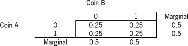
The joint distribution table shows the probability of all the outcomes when the two coins are tossed. In the case of two coin tosses there are 4 potential outcomes, hence there are 4 cells in the joint distribution table. For example, the probability of Coin A being a head (0) and Coin B a tail (1) can be determined by looking at the 0 row for Coin A and the 1 column for Coin B, in this example 0.25. In this case, our coins are independent. The correlation coefficient is zero, where we calculate the correlation coefficient by:

\[ \begin{array}{l} \text { Correlation Coefficient }\\ =\operatorname{Cov}(A, B) /(\operatorname{Stdev}(A) * \operatorname{Stdev}(B)) \end{array} \tag{2.1} \]

and

\[ \begin{aligned} \operatorname{Cov}(A, B) & =E[(A-\operatorname{mean}(A)) *(B-\operatorname{mean}(B))] \\ & =E(A B)-E(A) E(B) . \end{aligned} \tag{2.2} \]

We can also see that the outcomes of Coin B are not linked in any way to the outcome of Coin A. For example,

\[ \begin{aligned} P(B=1 \mid A=1) & =P(A=1, B=1) / P(A=1) \\ & =0.25 / 0.5 \\ & =0.50 \\ & =P(B=1) \end{aligned} \]

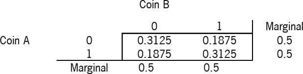
From this distribution we calculate the correlation coefficient to be 0.25.^[3]

By looking at the conditional distributions, it is clear that there is a link between the outcome of Coin B and Coin A:

\[ \begin{aligned} P(B=1 \mid A=1) & =P(A=1, B=1) / P(A=1) \\ & =0.3125 / 0.5 \\ & =0.625 \\ P(B=0 \mid A=1) & =0.375 \end{aligned} \]

So we can see that with the increase in correlation, there is an increase in the chance of getting heads on Coin B, given Coin A shows heads, and a corresponding decrease in the chance of getting tails on Coin B, given Coin A shows heads.

With this 2-coin example, it turns out that if we want the marginal distributions of each coin to be the standard 50% heads, 50% tails, then, given the correlation coefficient we want to produce, we can uniquely define the joint pdf for the coins.

We find that, for a given correlation coefficient of ρ,

\[ \begin{array}{l} P(A=1, B=1)=P(A=0, B=0)=(1+\rho) / 4 . \\ P(A=1, B=0)=P(A=0, B=1)=(1-\rho) / 4 . \end{array} \]

We can then recover the conditional probabilities:

\[ \begin{array}{l} P(B=1 \mid A=1)=(1+\rho) / 2 . \\ P(B=0 \mid A=1)=(1-\rho) / 2 . \end{array} \]

So, for example, we can see that

\[ \begin{array}{llll} \rho=0.00 & \text { gives } & P(B=1 \mid A=1)=0.500 . \\ \rho=0.50 & \text { gives } & P(B=1 \mid A=1)=0.750 . \\ \rho=0.75 & \text { gives } & P(B=1 \mid A=1)=0.875 . \\ \rho=1.00 & \text { gives } & P(B=1 \mid A=1)=1.000 . \end{array} \]

As expected, the more the correlation coefficient increases, the higher the chance of throwing heads on Coin B, given Coin A shows heads.

In lay terms, then, we would repeat our description of correlation at the start of this section, that correlation, or the “strength of relationship,” is a way of looking at the tendency of two variables, X and Y, to move in the same (or opposite) direction. As the coin example shows, the more positively correlated X and Y are, the greater our expectation that Y will be higher than average if X is higher than average.

It should be noted, however, that the expected value of the sum of two correlated variables is exactly equal to the expected value of the sum of the two uncorrelated variables with the same means.

In the context of actuarial reserving work, Brehm (2002) notes “the single biggest source of risk in an unpaid loss portfolio is arguably the potential distortions that can affect all open accident years, i.e., changes in calendar year trends” (p. 8). The real-life correlation issue that we are attempting to identify and resolve is the extent to which, if we see adverse (or favorable) development in ultimate losses in one line of business, we will see similar movement in other lines of business.

3. Significance of the existence of correlations between lines of business

Suppose we have two or more blocks of business for which we are trying to calculate reserve indications. If all we are trying to do is determine the expected value of the reserve run-off, we can calculate the expected value for each block separately and add all the expectations together. However, if we are trying to quantify a value other than the mean, such as the 75th percentile, we cannot simply sum across the lines of business. If we do so, we will overstate the aggregate reserve need. The only time the sum of the 75th percentiles would be appropriate for the aggregate reserve indication is when all the lines are fully correlated with each other—a highly unlikely situation! The degree to which the lines are correlated will influence the proper aggregate reserve level and the aggregate reserve range. How significant an impact will there be? That primarily depends upon two factors—how volatile the reserve ranges are for the underlying lines of business and how strongly correlated the lines are with each other. If there is not much volatility, then the strength of the correlation will not matter that much. If, however, there is considerable volatility, the strength of correlations will produce differences that could be material. This is demonstrated in the following example.

The impact on values at the 75th percentile as correlation and volatility increase.

Table 1 shows some figures relating the magnitude of the impact of correlations on the aggregate distribution to the size of the correlation. In this example, we have modeled two lines of business (A and B), assuming they were normally distributed with identical means and variances. The means were assumed to be 100 and the standard deviations were 25. We are examining the 75th percentile value derived for the sum of A and B. Table 1 shows the change in the 75th percentile value between the uncorrelated situation and varying levels of correlation between lines A and B. Reading down the column shows the impact of an increasing level of correlation between lines A and B, namely, that the ratio of the correlated to the uncorrelated value at the 75th percentile increases as correlation increases.

Now let’s expand the analysis to see what happens as the volatility of the underlying distributions increase. Table 2 shows a comparison of the sum of lines A and B at the 75th percentile as correlation increases and as volatility increases. The ratios in each column are relative to the value for the zero correlation value at each standard deviation value. For example, the 5.8% ratio for the rightmost column at the 25% correlation level means that the 75th percentile value for lines A+B with 25% correlation is 5.8% higher than the 75th percentile of \(N(100,200)_A+N(100,200)_B\) with no correlation. As can be seen from this table, the greater the volatility, the larger the differential between the uncorrelated and correlated results at the 75th percentile.

This effect is magnified if we look at similar results further out on the tails of the distribution, for example, looking at the 95th percentiles, as is shown in Table 3.

Note that these results will also depend on the nature of the underlying distributions—we would expect different results for lines of business that were lognormally distributed, for example.

4. Case study

4.1. Background

The data used in this case study is fictional. It describes three lines of business, two long-tail and one short-tail. All three produce approximately the same mean reserve indication, but with varying degrees of volatility around their respective means. By having the three lines of approximately equal size, we are able to focus on the impact of correlations between lines without worrying about whether the results from one line are overwhelming the results from the other two lines. Appendix I contains the data triangles.

The examination of the impact of correlation on the aggregated results will be done using two methods. The first assumes the person doing the analysis can provide a positive-definite correlation matrix (see section 4.2 below). The relationships described in the correlation matrix are used to convert the uncorrelated aggregate reserve range into a correlated aggregate range. The process does not affect the reserve ranges of the underlying lines of business. It just influences the aggregation of the reserve indications by line so that if two lines are positively correlated and the first line produces a reserve indication that is higher than the expected reserve indication for that line, it is more likely than not that the second line will also produce a reserve indication that is higher than its expected reserve indication. This is exactly what was demonstrated in the examples in Section 3.

The second method dispenses with what the person doing the analysis knows or thinks he knows. This method relies on the data alone to derive the relationships and linkages between the different lines of business. More precisely, this method assumes that all we need to know about how related the different lines of business are to each other is contained in the historical claims development that we have already observed. This method uses a technique known as bootstrapping to extract the relationships from the observed claims history. The bootstrapped data is used to generate reserve indications that inherently contain the same correlations that existed in the original data. Therefore, the aggregate reserve range is reflective of the underlying relationships between the individual lines of business, without first requiring the potentially messy step of requiring the person doing the analysis to develop a correlation matrix.

4.2. A note on the nature of the correlation matrix used in the analysis

The entries in the correlation matrix used must fulfill certain requirements that cause the matrix to be what is known as positive definite. The mathematical description of a positive definite matrix is that, given a vector x and a matrix A, where

\[ \begin{aligned} x & =\left[\begin{array}{lll} x_{1} & x_{2} & \cdots \\ a_{n} \end{array}\right] \\ A & =\left[\begin{array}{cccc} a_{11} & a_{12} & \cdots & a_{1 n} \\ a_{21} & a_{22} & \cdots & a_{2 n} \\ \vdots & \vdots & \cdots & \vdots \\ a_{n 1} & a_{n 2} & \cdots & a_{n n} \end{array}\right] \\ x^{T} A x & =\left[\begin{array}{lll} x_{1} & x_{2} & \cdots \\ a_{21} & a_{22} \end{array}\right]\left[\begin{array}{ccc} a_{11} & a_{12} & \cdots \\ \vdots & \vdots & \cdots \\ a_{n 1} & a_{n 2} & \cdots \\ a_{1 n} \end{array}\right]\left[\begin{array}{c} a_{2 n} \\ x_{2} \\ \vdots \\ x_{n} \end{array}\right] \\ & =a_{11} x_{1}^{2}+a_{12} x_{1} x_{2}+a_{21} x_{2} x_{1}+\cdots+a_{n n} x_{n}^{2} . \end{aligned} \tag{4.1} \]

\[\begin{align} &\text{Matrix A is positive definite when} \ x^{T} A x>0 \\ &\text{for all} \ x \ \text{other than} \ x_{1}=x_{2}=\cdots=x_{n}=0. \end{align}\tag{4.2} \]

In the context of this paper, matrix A is the correlation matrix we want to develop and the \(a_{ij}\) are the correlation coefficients.

4.3. Correlation matrix methodology

The methodology used in this approach is that of rank correlation. Rank correlation is a useful approach to dealing with two or more correlated variables when the joint distribution of the correlated variables is not normal. When using rank correlation, what matters is the ordering of the simulated outcomes from each of the individual distributions, or, more properly, the re-ordering of the outcomes.

4.3.1. Rank correlation example

Suppose we have two random variables, A and B. A and B are both defined by uniform distributions ranging from 100 to 200. Suppose we draw five values at random from A and B. They might look as shown in Table 4.

Now suppose we are interested in the joint distribution of A+B. We will use rank correlation to learn about this joint distribution. We will use a bivariate normal distribution to determine which value from distribution B ought to be paired with a value from distribution A. The easiest cases are when B is perfectly correlated with A or perfectly inversely correlated with A. In the perfectly correlated case, we pair the lowest value from A with the lowest value from B, the second lowest value from A with the second lowest value from B, and so on to the highest values for A and B. In the case of perfect inverse correlation, we pair the lowest value from A with the highest value from B, etc. The results from these two cases are shown in Table 5.

When there is no correlation between A and B, the ordering of the values from distribution B that are to be paired with values from distribution A are wholly random. The original order of the values drawn from distributions A and B is one example of the no-correlation condition. When positive correlations exist between A and B, the orderings reflect the level of correlation, and the range of the joint distribution will be somewhere between the wholly random situation and the perfectly correlated one.

4.3.2. Application of rank correlation methodology to reserve analysis

The application of the rank correlation methodology to a stochastic reserve analysis is done through a two-step process. In the first step, a stochastic reserving technique is used to generate N possible reserve runoffs from each data triangle being analyzed. It is important that a relatively large N value be used so as to capture the variability inherent in each data triangle, yet produce results that reasonably reflect the infrequent nature of highly unlikely outcomes. If too few outcomes are produced from each data triangle, the user risks either not producing results with sufficient variability or overstating the variability that does exist in the data. Examples of several different techniques, including bootstrapping (England 2001), application of the chain-ladder to logarithmically adjusted incremental paid data (Christofides 1990), and application of the chainladder to logarithmically adjusted cumulative paid data (Feldblum, Hodes, and Blumsohn 1999), can be found in articles listed in the bibliography to this paper. In this case study, 5,000 different reserve runoffs were produced using the bootstrapping technique described in England (2001). This is the end of step one.

In step two, the user must specify a correlation matrix, in which the individual elements of the correlation matrix (the \(a_{ij}\) described in Section 2) describe the pair-wise relationships between different pairs of lines being analyzed. We do not propose to cover how one may estimate such a correlation matrix in this paper, as we feel this is an important topic in its own right, the details of which would merit a separate paper. One such paper for readers who are looking for guidance in this area is Brehm (2002). In this paper, we will simply assume that the user has such a matrix, either calculated analytically or estimated using some other approach, such as a judgmental estimation of correlation.

We generate 5,000 samples for each line of business from a multivariate normal distribution, with the correlation matrix specified by the user. A discussion of how one might create these samples is contained in Appendix 2. We then sort the samples from the reserving method into the same rank order as the normally distributed samples. This ensures that the rank order correlations between the three lines of business are the same as the rank order correlations between the three normal distributions. The aggregate reserve distribution is calculated from the sum of the individual line reserve distributions. This resulting aggregate reserve range will be composed of 5,000 different values from which statistics such as the 75th percentile can be drawn. The range of aggregated reserve indications is reflective of the correlations entered into the correlation matrix at the start of the analysis.

For example, the ranked results from the multivariate normal process might be as follows:

The first of the 5,000 values in the aggregate reserve distribution will be composed of the 528th largest reserve indication for line 1 plus the 533rd largest reserve indication for line 2 plus the 400th largest reserve indication for line 3. The second of the 5,000 values will be composed of the 495th largest reserve indication for line 1 plus the 607th largest reserve indication for line 2 plus the 404th largest reserve indication for line 3. Through this process, the higher the positive correlation between lines, the more likely it is that a value below the mean for one line will be combined with a value below the mean for a second line. At the same time, the mean of the overall distribution remains unchanged and the distributions of the individual lines remains unchanged.

4.4. Rank correlation results

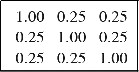
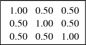
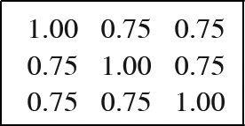
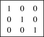
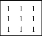
To show the impact of the correlations between the lines on the aggregate distribution, we ran the model five times, each time with different correlation matrices: zero correlation, 25% correlation, 50% correlation, 75% correlation, and 100% correlation. Specifically, the five correlation matrices were as follows:

1. Zero correlation:

2. 25% correlation:

3. 50% correlation:

4. 75% correlation:

5. 100% correlation:

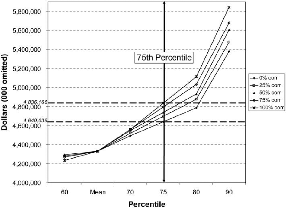
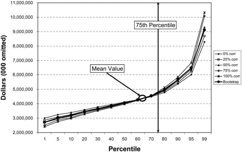
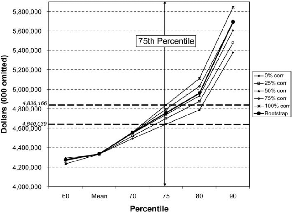
The correlations were chosen to highlight the range of outcomes that result for different levels of correlation, not because the data necessarily implied the existence of correlations such as these. The results are shown both numerically in Table 6 and graphically in Figure 1 and Figure 2.

As expected, the higher the positive correlation, the wider the aggregated reserve range. With increasingly higher positive correlations, it is less likely that a better-than-expected result in one line will be offset by a worse-than-expected result in another line. This causes the higher positive correlated situations to have lower aggregate values for percentiles below the mean and higher aggregate values for percentiles above the mean. The results of the table and graph show just this situation. For information purposes, the difference between the zero correlation situation and the perfectly correlated situation at the 75th percentile have been displayed in Figure 2.

4.5. Bootstrap methodology

Bootstrapping is a sampling technique that is an alternative to traditional statistical methodologies. In traditional statistical approaches, one might look at a sample of data and postulate the underlying distribution that gave rise to the observed outcomes. Then, when analyzing the range of possible outcomes, new samples are drawn from the postulated distribution. Bootstrapping, by comparison, does not concern itself with the underlying distribution. The bootstrap says that all the information needed to create new samples lies within the variability that exists in the already observed historical data. When it comes time to create the new samples, different observed variability factors are combined with the observed data to create “pseudodata” from which the new samples are generated.

So what is bootstrapping, then, as it is applied to reserve analysis? Bootstrapping is a resampling method that is used to estimate in a structured manner the variability of a parameter. In reserve analysis, the parameter is the difference between observed and expected paid amounts for any given accident year/development year combination. During each iteration of the bootstrapping simulation, random draws are made from all the available variability parameters. One random draw is made for each accident year/development year combination. The variability parameter is combined with the actual observation to develop a “pseudohistory” paid loss triangle. A reserve indication is then produced from the pseudohistory data triangle by applying the traditional cumulative chain-ladder technique to “square the triangle.” A step-by-step walkthrough of the bootstrap process is included in Appendix 2.

Note that this example is using paid amounts. The bootstrap approach can equally be applied to incurred data, to generate “pseudohistory” incurred loss triangles, which may be developed to ultimate in the same manner as the paid data. Also, the methodology is not limited to working with just positive values. This is an important capability when using incurred data, as negative incrementals will be much more common when working with incurred data.

This approach is extended to multiple lines in the following manner. Instead of making random draws of the variability parameters independently for each line of business, the same draws are used across all lines of business. The variability parameters will differ from line to line, but the choice of which variability parameter to pick is the same across lines.

The example of Table 7 through Table 9 should clarify the difference between the uncorrelated and correlated cases. The example shows two lines of business, Line A and Line B. Both are 4 × 4 triangles. Table 7 shows the variability parameters calculated from the original data. We start by labeling each parameter with the accident year, development year, and triangle from which the parameters are derived.

Table 8 shows one possible way the variability parameters might be reshuffled to create an uncorrelated bootstrap. For each Accident/Development year in each triangle A and B, we select a variability parameter from Table 7 at random. For example, Triangle A, Accident Year 1, Development Year 1 has been assigned (randomly) the variability parameter from the original data in Table 7, Accident Year 2, Development Year 1. Note that each triangle uses the variability parameters calculated from that triangle’s data, i.e., none of the variability parameters from Triangle A are used to create the pseudohistory in Triangle B. Also note that the choice of variability parameters for each Accident Year/Development Year in Triangle A is independent of the choice of variability parameter for the corresponding Accident Year/Development Year in Triangle B.

For the correlated bootstrap shown in Table 9, the choice of variability parameter for each Accident Year/Development Year in Triangle A is not independent of the choice of variability parameter for the corresponding Accident Year/Development Year in Triangle B. We ensure that the variability parameter selected from Triangle B comes from the same Accident Year/Development Year used to select a variability parameter from Triangle A.

The process shown in Table 9 implicitly captures and uses whatever correlations existed in the historical data when producing the pseudohistories from which the reserve indications will be developed. The resulting aggregated reserve indications will reflect the correlations that existed in the actual data, without requiring the analyst to first postulate what those correlations might be. This method also does not require the second stage reordering process that the correlation matrix methodology required. The correlated aggregate reserve indication can be derived in one step.

4.6. Bootstrap results

The model was run one final time using the bootstrap methodology to develop an aggregated reserve range. The bootstrap results have been added to the results shown in Table 6 and Figures 1 and 2. The revised results are shown in Table 10 and Figures 3 and 4, where we can compare the aggregate reserve distributions generated from the two different approaches.

The results shown in the preceding figures and tables provide us with the following information:

1. If we wanted to hold reserves at the 75th percentile, the smallest reserve that ought to be held is $4.640 billion and the largest ought to be $4.836 billion.

2. The maximum impact on the 75th percentile of indicated reserves due to correlation is 4.5% of the mean indication ($196 million/$4.331 billion).

3. There does appear to be correlation between at least two of the lines. The observed level of correlation is similar to what would be displayed were there to be a 50% correlation between each of the lines. It could be that two of the lines exhibit a stronger than 50% correlation with each other and a weaker than 50% correlation with the third line, so that the overall results produce values similar to what would exist at the 50% correlation level.

4. The reserve to book, assuming the 50% correlation is correct, is $4.739 billion. Alternatively, if we were to select the booked reserve based on the bootstrap methodology, the reserve to book is $4.755 billion.

Some level of correlation between at least two of the lines is indicated by the bootstrapped results. This is valuable information to know, even beyond the range of reserves indicated by the bootstrap methodology. With this information, company management can assess prospective underwriting strategies that recognize the interrelated nature of these lines of business, such as how much additional capital might be required to protect against adverse deviation. If the lines were uncorrelated, future adverse deviation in one line would not necessarily be reflected in the other lines. With the information at hand, it would be inappropriate to assume that adverse deviation in one line will not be mirrored by adverse deviation in one or both of the other lines. Continuing with this thought, the bootstrapped results would have been valuable even if they had shown there to be little or no correlation between the lines—because then company management could comfortably assume independence between the lines of business and make their strategic decisions accordingly.

5. Summary and conclusions

Let us move beyond the numbers of the case study to summarize what we feel to be the important general conclusions that can be drawn. To begin, calculating an aggregate reserve distribution for several lines of business requires not only a model for the distribution of reserves for each individual line of business, but also an understanding of the dependency of the reserve amounts between each of the lines of business. To get a feel for the impact of these dependencies on the aggregate distribution, we have proposed two different methods. One can use a rank correlation approach with correlation parameters estimated externally. However, this approach requires either calculating correlations using a method such as has been proposed by Brehm (2002) or by judgmentally developing a correlation matrix. Alternatively, one can use a bootstrap method that relies on the existing dependencies in the historic data triangles. This requires no external calibration, but may be less transparent in providing an understanding of the data. It also limits the calculations to reflecting only those relationships that have existed in the past in the projection of reserve indications.

Additionally, a user of either method is cautioned to understand actions taken by the company that might create a false impression of strong correlation across lines of business. For example, if a company changes its claim reserving or settlement philosophy, we would expect to see similar impacts across all lines of business. To a user not aware of this change in company philosophy, it could appear that there are strong underlying correlations across lines of business when in reality there might not be.

Furthermore, it would appear that the correlation issue is not important for lines of business with nonvolatile reserve ranges. However, for volatile reserves, the impact of correlations between lines of business could be significant, particularly as one moves towards more extreme ends of the reserve range. If so, either correlation approach can provide actuaries with a way of quantifying the effect of correlations on the aggregate reserve range. Overall, the use of stochastic techniques adds value, as such techniques can not only assess the volatility of reserves, but also identify the significance of correlations between lines of business in a more rigorous manner than is possible with traditional techniques.

To conclude, we believe that stochastic quantification of reserve ranges, with or without an analysis of correlations between lines of business, is a valuable extension of current actuarial practice. Regulations such as those recently promulgated by APRA will accelerate the general usage of stochastic techniques in reserve analysis. An accompanying benefit to the use of stochastic reserving techniques is the ability to quantify the effects of correlations between lines of business on overall reserve ranges. This will help actuaries and company management to better understand how variable reserve development might be, both by line and in the aggregate, allowing companies to make better-informed decisions on the booking of reserves and the amount of capital that must be deployed to protect the company against adverse reserve development.