Bootstrap Estimation of the Predictive Distributions of Reserves Using Paid and Incurred Claims

undefined

1. Introduction

Bootstrapping has become very popular in stochastic claims reserving because of the simplicity and flexibility of the approach. One of the main reasons for this is the ease with which it can be implemented in a spreadsheet in order to obtain an approximation to the estimation error of a fitted model in a statistical context. Furthermore, it is also straightforward to extend it to obtain the approximation to the prediction error and the predictive distribution of a statistical process by including simulations from the underlying distributions. Therefore, bootstrapping is a powerful tool for the most popular subject for reserving purposes in general insurance, the prediction error of the reserve estimates. It should be emphasized that to obtain the predictive distribution, rather than just the estimation error, it is necessary to extend the bootstrap procedure by simulating the process error. It is also important to realize that bootstrapping is not a “model,” and therefore it is important to ensure that the underlying reserving models are correctly calibrated to the observed data. In this paper, we do not address the issue of model checking, but simply show how a bootstrapping procedure can be applied to the Munich chain ladder model.

In the area of non-life insurance reserving, there are primarily two types of data used. In addition to the paid claims triangle, there is frequently a triangle of incurred data also available. The traditional approach is to fit a model to either paid or incurred claims data separately, and one of the most popular methods in this context is the chain ladder technique. While we do not believe that this is the most appropriate approach for all data sets, it has retained its popularity for a number of reasons. For example, the parameters are understood in a practical context; it is flexible; and it is easy to apply. This paper concentrates on methods which have a chain ladder structure, and in this context, two types of approaches exist: deterministic methods such as chain ladder, and the recently developed stochastic chain ladder reserving models. When the chain ladder technique is used (either as a deterministic approach or using a stochastic model), one set of data will be omitted—either the paid or the incurred data can be used, but not both at the same time. Obviously, this does not make full use of all the data available and results in the loss of some information contained in those data.

This leads us to consider whether it is possible to construct a model for both data sets, and to a consideration of the dependency between the two run-off triangles. A related issue also arises when traditional methods are applied separately to each triangle, which produces inconsistent predicted ultimate losses. In response, Quarg and Mack (2004) proposed a different approach within a regression framework, considering the likely correlations between paid and incurred data. Quarg and Mack (2004) called this new method the Munich chain ladder (MCL) model. It is this model that is the subject of this paper, and we show how the predictive distribution may be estimated using bootstrapping. Thus, in this paper an adapted bootstrap approach is described, combined with simulation for two dependent data sets. The spreadsheets used in this paper can be used in practice for any data sets and are available on request from the authors.

The paper is set out as follows. Section 2 briefly describes the MCL model using a notation appropriate for this paper. In Section 3, the basic algorithm and methodology of bootstrapping is explained. Section 4 shows how to obtain the estimates of the prediction errors and the empirical predictive distribution using the adapted bootstrapping and simulation methods. In Section 5, two numerical examples are provided, including the data from Mack (1993) as well as some real London market data. Finally, Section 6 contains a discussion and conclusion.

2. The Munich chain ladder method

The MCL model aims to produce a more consistent prediction of ultimate claims when modeling both paid and incurred claim data. It is specially designed to deal with the correlation between paid and incurred claims. The traditional models, such as the chain ladder model, sometimes produce unsatisfactory results by ignoring this dependence. It should be emphasized that the paid and incurred claims from the same calendar years are not correlated. It is that the paid claims (incurred claims) are correlated with the incurred claims (paid claims) from the next (previous) calendar year.

The fundamental structure of the MCL model is the same as Mack’s distribution-free chain ladder model (Mack 1993). In other words, the chain ladder development factors in the MCL model are obtained by Mack’s distribution-free approach. However, the MCL model adjusts the chain ladder development factors using the correlations between the observed paid and incurred claims. The adjusted chain ladder development factors therefore become individual not only for different development years but also for different accident years. The adjustment is explained in more detail in Sections 2.1 and 2.2.

2.1. Notation and assumptions

For ease of notation, we assume that we have a triangle of data. Although the data could be classified in different ways, we refer to the rows as “accident years” and the columns as “development years.”

Denote $C_{i j}^P$ as cumulative paid claims and $C_{i j}^I$ as cumulative incurred claims occurred in accident year $i$, development year $j$, where $1 \leq i \leq n$ and $1 \leq j \leq n-i+1$ for the observed data. The aim of the chain ladder technique and of MCL is to estimate the data up to development year $n$. This produces estimates for $C_{i j}^P$ and $C_{i j}^I$, where $1 \leq i \leq n$ and $n-i+2 \leq j \leq n$, and we thereforerefer to the complete rectangle of data in the assumptions: $1 \leq i, j \leq n$.

Mack’s distribution-free chain ladder method models the pattern of the development factors, which are defined as $F_{i j}^P=C_{i, j+1}^P / C_{i j}^P$, for paid claims and $F_{i j}^I=C_{i, j+1}^I / C_{i j}^I$, for incurred claims. Also the ratios of paid divided by incurred claims and the inverse are introduced as $Q_{i j}=C_{i j}^P / C_{i j}^I$ and $Q_{i j}^{-1}=C_{i j}^I / C_{i j}^P$, respectively.

Furthermore, define the observed data for accident year $i$, up to development year $k$ as $P_i(k)$ $=\left\{C_{i j}^P: j \leq k\right\}, I_i(k)=\left\{C_{i j}^I: j \leq k\right\}$ and $B_i(k)=$ $\left\{C_{i j}^P, C_{i j}^I: j \leq k\right\}$, for paid claims, incurred claims and both, respectively.

The following assumptions are taken from Quarg and Mack (2004), Section 2.1.2.

Assumption A (Expectations)

(A1) For $1 \leq j \leq n$ there exists a constant $f_j^P$ such that (for $i=1, \ldots, n$ )

$$E\left[F_{i j}^P \mid P_i(j)\right]=f_j^P.$$

This assumption is for paid claims. It is necessary to make another analogous assumption for incurred claims since both data sets are taken into account.

(A2) For $1 \leq j \leq n$, there exists a constant $f_j^I$ such that (for $i=1, \ldots, n$ )

$$E\left[F_{i j}^I \mid I_i(j)\right]=f_j^I.$$

In order to analyze the two run-off triangles dependently, the following assumptions are also required.

(A3) For $1 \leq j \leq n$, there exists a constant $q_j^{-1}$ such that (for $i=1, \ldots, n$ )

$$E\left[Q_{i j}^{-1} \mid P_i(j)\right]=q_j^{-1}.$$

(A4) For $1 \leq j \leq n$, there exists a constant $q_j$ such that (for $i=1, \ldots, n$ )

$$E\left[Q_{i j} \mid I_i(j)\right]=q_j.$$

Note that assumptions (A3) and (A4) will apply that imply that $Q_{i j}$ is constant, which is con-tradictory-see Section 3.1.2 of Quarg and Mack (2004) for a discussion of this point.

Assumption B (Variances)

(B1) For $1 \leq j \leq n$, there exists a constant $\sigma_j^P$ such that (for $i=1, \ldots, n$ )

$$\operatorname{Var}\left[F_{i j}^P \mid P_i(j)\right]=\frac{\left(\sigma_j^P\right)^2}{C_{i j}^P}.$$

Again, the analogous assumption for the incurred claims is made as follows.

(B2) For $1 \leq j \leq n$, there exists a constant $\sigma_j^I$ such that (for $i=1, \ldots, n$ )

$$\operatorname{Var}\left[F_{i j}^I \mid I_i(j)\right]=\frac{\left(\sigma_j^I\right)^2}{C_{i j}^I}.$$

Also, for the ratios of incurred to paid and vice versa, the following variance assumptions are made.

(B3) For $1 \leq j \leq n$, there exists a constant $\tau_j^P$ such that (for $i=1, \ldots, n$ )

$$\operatorname{Var}\left[Q_{i j}^{-1} \mid P_i(j)\right]=\frac{\left(\tau_j^P\right)^2}{C_{i j}^P}.$$

(B4) For $1 \leq j \leq n$, there exists a constant $\tau_j^I$ such that for $(i=1, \ldots, n)$

$$\operatorname{Var}\left[Q_{i j} \mid I_i(j)\right]=\frac{\left(\tau_j^I\right)^2}{C_{i j}^I} .$$

Assumption C (Independence)

Assumption $C$ (Independence) The usual assumptions for individual triangles are as follows:

(C1) The random variables pertaining to different accident years for paid claims, i.e., $\left\{C_{1 j}^P \mid\right.$ $j=1,2, \ldots, n\}, \ldots,\left\{C_{n j}^P \mid j=1,2, \ldots, n\right\}$, are stochastically independent.

(C2) The random variables pertaining to different accident years for incurred claims, i.e., $\left\{C_{1 j}^I \mid j=1,2, \ldots, n\right\}, \ldots,\left\{C_{n j}^I \mid j=1,2, \ldots, n\right\}$, are stochastically independent.

In fact, a stronger assumption is used (see Section 3.2 of Quarg and Mack 2004), which is independence of accident years across both paid and incurred claims:

(C3) The random sets $\left\{C_{1 j}^P, C_{1 j}^I \mid j=1,2, \ldots, n\right\}$ $, \ldots,\left\{C_{n j}^P, C_{n j}^I \mid j=1,2, \ldots, n\right\}$, are stochastically independent.

Using assumptions A to C, the Pearson residuals used in the MCL model can be defined as shown in Equations (2.1) to (2.4). These residuals are a crucial part of the bootstrapping procedures described in Section 4.

$$r_{i j}^{P}=\frac{F_{i j}^{P}-E\left[F_{i j}^{P} \mid P_{i}(j)\right]}{\sqrt{\operatorname{Var}\left[F_{i j}^{P} \mid P_{i}(j)\right]}}, \tag{2.1}$$

$$r_{i j}^{Q^{-1}}=\frac{Q_{i j}^{-1}-E\left[Q_{i j}^{-1} \mid P_{i}(j)\right]}{\sqrt{\operatorname{Var}\left[Q_{i j}^{-1} \mid P_{i}(j)\right]}}, \tag{2.2}$$

$$r_{i j}^{I}=\frac{F_{i j}^{I}-E\left[F_{i j}^{I} \mid I_{i}(j)\right]}{\sqrt{\operatorname{Var}\left[F_{i j}^{I} \mid I_{i}(j)\right]}}, \tag{2.3}$$

$$r_{i j}^{Q}=\frac{Q_{i j}-E\left[Q_{i j} \mid I_{i}(j)\right]}{\sqrt{\operatorname{Var}\left[Q_{i j} \mid I_{i}(j)\right]}} . \tag{2.4}$$

Assumption D (Correlations)

(D1) There exists a constant $\rho^P$ such that (for $1 \leq i, j \leq n$ )

$$E\left[r_{i j}^P \mid B_i(j)\right]=\rho^P r_{i j}^{Q^{-1}} .\tag{2.5}$$

The following equation states that the constant $\rho^P$ is in fact the correlation coefficient between the residuals. Note that since the residuals have variance 1 , the correlation is equal to the covariance. The proof can be found in Quarg and Mack (2004).

$$\begin{aligned} \operatorname{Cov}\left[r_{i j}^{P}, r_{i j}^{Q^{-1}} \mid P_{i}(j)\right] & =\operatorname{Corr}\left[r_{i j}^{P}, r_{i j}^{Q^{-1}} \mid P_{i}(j)\right] \\ & =\operatorname{Corr}\left[F_{i j}^{P}, Q_{i j}^{-1} \mid P_{i}(j)\right]=\rho^{P} \end{aligned} \tag{2.6}$$

Quarg and Mack (2004) derives expected MCL paid development factors adjusted by the correlation as shown in Equation (2.7).

$$\begin{aligned} E\left[F_{i j}^{P} \mid\right. & \left.B_{i}(j)\right] \\ = & E\left[F_{i j}^{P} \mid P_{i}(j)\right]+\sqrt{\frac{\operatorname{Var}\left[F_{i j}^{P} \mid P_{i}(j)\right]}{\operatorname{Var}\left[Q_{i j}^{-1} \mid P_{i}(j)\right]}} \\ & \times \operatorname{Corr}\left[F_{i j}^{P}, Q_{i j}^{-1} \mid B_{i}(j)\right]\left(Q_{i j}^{-1}-E\left[Q_{i j}^{-1} \mid P_{i}(j)\right]\right). \end{aligned} \tag{2.7}$$

(D2) Analogous to assumption (D1), for the incurred claims it is assumed that there exists a constant $\rho^I$ such that (for $1 \leq i, j \leq n$ )

$$E\left[r_{i j}^{I} \mid B_{i}(j)\right]=\rho^{I} r_{i j}^{Q}. \tag{2.8}$$

Similarly, the constant $\rho^I$ measures the correlation coefficient or the covariance between the residuals. i.e.,

$$\begin{aligned} \operatorname{Cov}\left[r_{i j}^{I}, r_{i j}^{Q} \mid B_{i}(j)\right] & =\operatorname{Corr}\left[r_{i j}^{I}, r_{i j}^{Q} \mid B_{i}(j)\right] \\ & =\operatorname{Corr}\left[F_{i j}^{I}, Q_{i j} \mid B_{i}(j)\right]=\rho^{I} \end{aligned} \tag{2.9}$$

Hence, the expected MCL incurred development factors adjusted by the correlation can be derived as follows:

$$\begin{aligned} E\left[F_{i j}^{I} \mid\right. & \left.B_{i}(j)\right] \\ = & E\left[F_{i j}^{I} \mid I_{i}(j)\right]+\sqrt{\frac{\operatorname{Var}\left[F_{i j}^{I} \mid I_{i}(j)\right]}{\operatorname{Var}\left[Q_{i j} \mid I_{i}(j)\right]}} \\ & \times \operatorname{Cov}\left[F_{i j}^{I}, Q_{i j} \mid B_{i}(j)\right]\left(Q_{i j}-E\left[Q_{i j} \mid I_{i}(j)\right]\right). \end{aligned} \tag{2.10}$$

2.2. Unbiased estimates of the parameters

In this section, we summarize the unbiased estimates of the parameters derived by Quarg and Mack (2004). For the paid data, estimates are required for the parameters of the development factors, the variances and also the correlation coefficient.

The estimates of the paid development factor parameters can be interpreted as weighted averages of the observed development factors $F_{i j}^P$ or $Q_{i j}^{-1}$, using $C_{i j}^P$ as the weights

$$\hat{f}_{j}^{P}=\frac{\sum_{i=1}^{n-j} C_{i, j+1}^{P}}{\sum_{i=1}^{n-j} C_{i j}^{P}}=\sum_{i=1}^{n-j} \frac{C_{i j}^{P}}{\sum_{i=1}^{n-j} C_{i j}^{P}} F_{i j}^{P} \tag{2.11}$$

and

$$\hat{q}_{j}^{-1}=\frac{\sum_{i=1}^{n-j+1} C_{i j}^{I}}{\sum_{i=1}^{n-j+1} C_{i j}^{P}}=\sum_{i=1}^{n-j+1} \frac{C_{i j}^{P}}{\sum_{i=1}^{n-j+1} C_{i j}^{P}} Q_{i j}^{-1} . \tag{2.12}$$

The unbiased estimates of the variances are as follows:

$$\left(\hat{\sigma}_{j}^{P}\right)^{2}=\frac{1}{n-j-1} \sum_{i=1}^{n-j} C_{i j}^{P}\left(F_{i j}^{P}-\hat{f}_{j}^{P}\right)^{2} \tag{2.13}$$

and

$$\left(\hat{\tau}_{j}^{P}\right)^{2}=\frac{1}{n-j} \sum_{i=1}^{n-j+1} C_{i j}^{P}\left(Q_{i j}^{-1}-\hat{q}_{j}^{-1}\right)^{2} \tag{2.14}$$

Hence the Pearson residuals are

$$r_{i j}^{P}=\frac{F_{i j}^{P}-\hat{f}_{j}^{P}}{\hat{\sigma}_{j}^{P}} \sqrt{C_{i j}^{P}} \tag{2.15}$$

and

$$r_{i j}^{Q^{-1}}=\frac{Q_{i j}^{-1}-\hat{q}_{j}^{-1}}{\hat{\tau}_{j}^{P}} \sqrt{C_{i j}^{P}}. \tag{2.16}$$

Finally, the estimate of the correlation coefficient is given in Equation (2.17).

$$\hat{\rho}^{P}=\frac{\sum_{i, j} r_{i j}^{Q^{-1}} r_{i j}^{P}}{\sum_{i, j}\left(r_{i j}^{Q^{-1}}\right)^{2}}. \tag{2.17}$$

Similarly, for incurred data, the estimates of the development factor parameters can be interpreted as weighted averages of the development factors $F_{i j}^I$ or $Q_{i j}$, using $C_{i j}^I$ as the weights:

$$\hat{f}_{j}^{I}=\frac{\sum_{i=1}^{n-j} C_{i, j+1}^{I}}{\sum_{i=1}^{n-j} C_{i j}^{I}}=\sum_{i=1}^{n-j} \frac{C_{i j}^{I}}{\sum_{i=1}^{n-j} C_{i j}^{I}} F_{i j}^{I} \tag{2.18}$$

and

$$\hat{q}_{j}=\frac{\sum_{i=1}^{n-j+1} C_{i j}^{P}}{\sum_{i=1}^{n-j+1} C_{i j}^{I}}=\sum_{i=1}^{n-j+1} \frac{C_{i j}^{I}}{\sum_{i=1}^{n-j+1} C_{i j}^{I}} Q_{i j}. \tag{2.19}$$

Also, the unbiased estimates for the variance parameters are as follows:

$$\left(\hat{\sigma}_{j}^{I}\right)^{2}=\frac{1}{n-j-1} \sum_{i=1}^{n-j} C_{i j}^{I}\left(F_{i j}^{I}-\hat{f}_{j}^{I}\right)^{2}. \tag{2.20}$$

and

$$\left(\hat{\tau}_{j}^{I}\right)^{2}=\frac{1}{n-j} \sum_{i=1}^{n-j+1} C_{i j}^{I}\left(Q_{i j}-\hat{q}_{j}\right)^{2}. \tag{2.21}$$

Hence the Pearson residuals are

$$r_{i j}^{I}=\frac{F_{i j}^{I}-\hat{f}_{j}^{I}}{\hat{\sigma}_{j}^{I}} \sqrt{C_{i j}^{I}} \tag{2.22}$$

and

$$r_{i j}^{Q}=\frac{Q_{i j}-\hat{q}_{j}}{\hat{\tau}_{j}^{I}} \sqrt{C_{i j}^{I}}. \tag{2.23}$$

And finally, the estimate of the correlation coefficient is given in Equation (2.24).

$$\hat{\rho}^{I}=\frac{\sum_{i, j} r_{i j}^{Q} r_{i j}^{I}}{\sum_{i, j}\left(r_{i j}^{Q}\right)^{2}}. \tag{2.24}$$

Assumptions A in Section 2.1 have defined the expectations of the development factors, given just the data in the respective triangles. In order to produce a single estimate based on the data from both paid and incurred data, Quarg and Mack (2004) also considers the expectations of the development factors given both triangles, and defines $E\left[F_{i j}^P \mid B_i(j)\right]=\lambda_{i j}^P$ and $E\left[F_{i j}^I \mid B_i(j)\right]$ $=\lambda_{i j}^I$. Using plug-in estimates from Equations (2.11) to (2.17), the estimates of the paid MCL development factors are calculated using Equation (2.7):

$$\hat{\lambda}_{i j}^{P}=\hat{f}_{j}^{P}+\hat{\rho}^{P} \frac{\hat{\sigma}_{j}^{P}}{\hat{\tau}_{j}^{P}}\left(Q_{i j}^{-1}-\hat{q}_{j}^{-1}\right) . \tag{2.25}$$

Similarly, plug-in estimates from Equations (2.18) to (2.24) are used in Equation (2.10) so that the estimates of the incurred development factors are

$$\hat{\lambda}_{i j}^{I}=\hat{f}_{j}^{I}+\hat{\rho}^{I} \frac{\hat{\sigma}_{j}^{I}}{\hat{\tau}_{j}^{I}}\left(Q_{i j}-\hat{q}_{j}\right) .\tag{2.26}$$

3. Bootstrapping and claims reserving

Bootstrapping is a simulation-based approach to statistical inference. It is a method for producing sampling distributions for statistical quantities of interest by generating pseudo samples, which are obtained by randomly drawing, with replacement, from observed data. It should be emphasized that bootstrapping is a method rather than a model. Bootstrapping is useful only when the underlying model is correctly fitted to the data, and bootstrapping is applied to data which are required to be independent and identically distributed. The bootstrapping method was first introduced by Efron (1979) and a good introduction to the algorithm can be found in Efron and Tibshirani (1993).

For the purpose of clarity we begin by giving a general bootstrapping algorithm and briefly reviewing previous applications of bootstrapping to claims reserving. In Section 4., we show how an algorithm of this type can be applied to the MCL. Suppose we have a sample and we require the distribution of a statistic θ̂. The following three steps comprise the simplest bootstrapping process:

1. Draw a bootstrap sample $\vec{X}_1^B=\left\{X_1^B, X_2^B, \ldots\right.$, $\left.X_n^B\right\}_1$ from the observed data $\vec{X}=\left\{X_1, X_2, \ldots\right.$, $\left.X_n\right\}$.
2. Calculate the statistic of interest $\hat{\theta}_1^B$ for the first bootstrap sample $\vec{X}_1^B=\left\{X_1^B, X_2^B, \ldots, X_n^B\right\}_1$.
3. Repeat steps 1 and $2 N$ times.

By repeating steps 1 and $2 N$ times, we obtain a sample of the unknown statistic $\hat{\theta}$, calculated from $N$ pseudo samples, i.e., $\vec{\theta}^B=\left\{\hat{\theta}_1^B, \hat{\theta}_2^B, \ldots, \hat{\theta}_N^B\right\}$. When $N \geq 1000$, the empirical distribution constructed from $\vec{\theta}^B=\left\{\hat{\theta}_1^B, \hat{\theta}_2^B, \ldots, \hat{\theta}_N^B\right\}$ can be taken as the approximation to the distribution for the statistic of interest $\hat{\theta}$. Hence all the quantities of the statistic of interest $\hat{\theta}$ can be obtained, since such a distribution contains all the information related to $\hat{\theta}$.

The above bootstrapping algorithm can be applied to the prediction distributions for the best estimates in stochastic claims reserving. England and Verrall (2007) contains an excellent review of the application. In addition, Lowe (1994), England and Verrall (1999), and Pinheiro, Andrade e Silva, and Centeno (2003) are also good resources for more details. England and Verrall (2007) showed how bootstrapping can be used for recursive models, following from the earlier papers (England and Verrall 1999; England 2002) which applied bootstrapping to the overdispersed Poisson model.

It should be noted here that the Pearson residuals are commonly used rather than the original data in the generalized linear model (GLM) framework. The Pearson residuals are required in order to scale the response variables in the GLM so that they are identically distributed. This is necessary because the bootstrap algorithm requires that the response variables are independent and identically distributed.

Other papers in the actuarial literature that consider triangles of dependent data include Taylor and McGuire (2007) and Kirschner, Kerley, and Isaacs (2008). It should be noted here that a model taking account of all information available could be very valuable, even when the data is dependent in practice. The dependence makes it difficult to calculate the prediction error theoretically. For these reasons, we believe that adopting bootstrap method for these models is worthy of investigation, particularly in order to obtain the predictive distribution of the estimates of outstanding liabilities.

4. Bootstrapping the Munich chain ladder model

This section considers bootstrapping the MCL model. In Section 4.1 we describe the methodology and in Section 4.2 we give the algorithm that is used.

4.1. Methodology

The method of bootstrapping stochastic chain ladder models can be seen in a number of different contexts. England and Verrall (2007) categorize the models as recursive and nonrecursive and show how bootstrapping methods can be applied in either case. Since we are dealing with recursive models here, we follow England and Verrall and consider the observed development link ratios rather than the claims data themselves. In other words, for Mack’s distributionfree chain ladder model the link ratios $F_{i j}$ are randomly drawn against $X_{i j}$, noting that

$$E\left[F_{i j} \mid X_{i j}\right]=E\left[\left.\frac{X_{i, j+1}}{X_{i j}} \right\rvert\, X_{i j}\right]=f_{j}.$$

Here, $X_{i j}$ is used to represent observed claims data in general. Note that the bootstrap estimates of the development factors $f_j^B$ which are obtained by taking weighted averages of the bootstrapped observed link ratios $F_{i j}^B$, use $X_{i j}$ rather than $X_{i j}^B$ as the weights.

However, this method cannot be simply extended to the MCL method, since this model is designed for dealing with two sets of correlated data, the paid and incurred claims. This means that it is not possible to use the normal bootstrap approach because the independence assumption cannot be met.

In order to address the problem of how to adapt the existing bootstrap approach in order to cope with the MCL method for dependent data sets, the consideration of the correlation is crucial. It should be noted that the correlation which is observed in the data represents real dependence between the paid and incurred claims, and the model is specifically designed for this dependence. Therefore, it should remain unchanged within any resampling procedure. The straightforward solution is to draw samples pairwise so that the correlation between the two dependent original data sets will not be broken when generating a sampling distribution for a statistic of interest.

Obviously, when bootstrapping the recursive MCL method, the residuals of the paid and incurred link ratios are required instead of the raw data. The question arises of how to deal with these residuals in order to meet the requirement of not breaking the observed dependence between paid and incurred claims. The answer is to group all four sets of residuals calculated in the MCL method, i.e., the paid and incurred development link ratios, the ratios of incurred over paid claims from the previous years, and its inverse, individually. There are two reasons for this. First, the paid claims (incurred claims) are correlated to the incurred to the paid claims ratio (paid to incurred claims ratio) from the previous year, and doing this will preserve the required dependence. Second, the correlation coefficient of paid and incurred claims is equal to the correlation coefficient of those residuals, as stated in Equations (2.6) and (2.10).

Thus, in the case of the paid claims data, the triangles (which have the same dimensions) containing the residuals of the observed paid link ratios and the residuals of the ratios of incurred over paid (except the first column), are paired together. The same procedure is used for the incurred claims data. We do this for convenience, even though the ratios of the paid over incurred claims and the inverse give the same information. Note that these ratios should remain unchanged when pairing them with paid and incurred claims with the same dimensions. The consequence of this is that all four sets of residuals for paid, incurred link ratios and the ratios of incurred over paid claims and the inverse are all grouped together. (Note here that an alternative approach would be to group three sets of residuals: the residuals of the paid and incurred link ratios and either the residuals of the paid over incurred ratios or the inverse. This would produce the same results as grouping four sets of residuals, as the residuals of paid over incurred ratios and the inverse can always be calculated from each other. However, it is simpler to group the four sets, as the calculation of the fourth set of residuals is naturally skipped in this case.)

This combines the four residuals triangles into one new triangle that consists of these grouped residuals and we name it as the grouped residual triangle. In each unit from this triangle of quadruples, the residuals are from the same accident and development year and correspond to paid and incurred claims. Therefore, the new triangle of quadruples contains all the information available and meanwhile maintains the observed dependence.

When applying bootstrapping, this triangle is considered as the observed sample. The new generated pseudo samples are obtained by random drawing, with replacement, from the triangle of quadruples.

The resampled incurred and paid triangles can be obtained by separating the pairs in the pseudo sample generated as above and backing out the residual definition. The MCL approach can then be applied to calculate all the statistics of interest for the resampled paid and incurred triangles, i.e., the correlation coefficient for paid and incurred, the paid and incurred development factors, the ratios of paid over incurred or the inverse, and the variances. Finally, adjusting the paid and incurred development factors by the correlation coefficient using the MCL approach, the bootstrapped MCL reserve estimates are obtained. This completes a single bootstrap iteration.

Again, the bootstrap method provides only the estimation error of the MCL method. In order to include the prediction error and estimate the predictive distribution for the MCL estimates of outstanding liabilities, an additional step is added at the end of each bootstrap iteration, which is to add the process variance to the estimation error.

Note that we apply the final simulation for the process variance to paid and incurred claims independently. This is because, for a particular accident and development year, paid and incurred claims are actually independent. Under the assumptions of the MCL model, paid (incurred) claims are only correlated with previous incurred (paid) claims, and the forecasts produced by the bootstrapping will pick up this dependency.

In order to obtain a reasonable approximation to the predictive distribution, at least 1000 pseudo samples are required. For each of the pseudo samples, the row totals and overall total of outstanding liabilities are stored so that the sample means, sample variances, and the empirical distributions can be calculated and plotted. They are taken as the approximations to the best estimates of outstanding liabilities, the prediction errors, and the predictive distributions of the outstanding liabilities. Also, an estimate of any required percentile and confidence interval can be calculated from the predictive distribution.

In order to satisfy the assumption that the sample is identically distributed in the bootstrapping procedure, the Pearson residuals are calculated and used. As in England and Verrall (2007), we use the Pearson residuals of the observed development factors rather than those for the actual claims, since we are using recursive models. Note that a bootstrap bias correction is also needed, and the simplest way to do this is to multiply the residuals by $\sqrt{(n-j) /(n-j-1)}$.

In addition to drawing the grouped sample for bootstrapping correlated data sets, there are also two other practical points that should be mentioned. The first is to note that the fitted values are obtained by starting from the final diagonal in each triangle and working backwards, by dividing by the development factors. The second is that the zero residuals which appear in both triangles are also left out.

4.2. Algorithm

This section provides the algorithm, step by step, which is needed in order to implement the bootstrap process introduced in Section 4.1.

• Apply the MCL method to both the cumulative paid and incurred claims data to obtain the residuals for all four sets of ratios: the paid, incurred link ratios, the paid over incurred ratios, and the reverse. They can be obtained from following equations:

  $$\begin{aligned} r_{i j}^{P}& =\frac{F_{i j}^{P}-\hat{f}_{j}^{P}}{\hat{\sigma}_{j}^{P}} \sqrt{C_{i j}^{P}},\\ r_{i j}^{Q^{-1}} & =\frac{Q_{i j}^{-1}-\hat{q}_{j}^{-1}}{\hat{\tau}_{j}^{P}} \sqrt{C_{i j}^{P}}, \\ r_{i j}^{I} & =\frac{F_{i j}^{I}-\hat{f}_{j}^{I}}{\hat{\sigma}_{j}^{I}} \sqrt{C_{i j}^{I}} \quad \text { and } \\ r_{i j}^{Q} & =\frac{Q_{i j}-\hat{q}_{j}}{\hat{\tau}_{j}^{I}} \sqrt{C_{i j}^{I}} \end{aligned}$$

• Adjust the Pearson residual estimates by multiplying by $\sqrt{(n-j) /(n-j-1)}$ to correct the bootstrap bias.

• Group all four residuals together, i.e., $r_{i j}^P, r_{i j}^{Q^{-1}}$, $r_{i j}^I$ and $r_{i j}^Q$. We write this as $U_{i j}=\left\{\left(r_{i j}^P\right),\left(r_{i j}^{Q^{-1}}\right)\right.$, $\left.\left(r_{i j}^I\right),\left(r_{i j}^Q\right)\right\}$.

• Start the iterative loop to be repeated N times (N ≥ 1000). This consists of the following steps:

  1. Randomly sample from the grouped residuals with replacement, denoted as $U_{i j}^B=$ $\left\{\left(r_{i j}^P\right)^B,\left(r_{i j}^{Q^{-1}}\right)^B,\left(r_{i j}^I\right)^B,\left(r_{i j}^Q\right)^B\right\}$, from the grouped triangle so that a pseudo sample of the grouped residuals is created.

  2. Calculate the pseudo samples of the four triangles for the paid, incurred link ratios, the ratios of paid over incurred, and the inverse by inverting the Pearson residuals definition as follows:

     $$\begin{aligned} \left(F_{i j}^{P}\right)^{B} & =\frac{\left(r_{i j}^{P}\right)^{B} \hat{\sigma}_{j}^{P}}{\sqrt{C_{i, j}^{P}}}+\hat{f}_{j}^{P}, \\ \left(Q_{i j}^{-1}\right)^{B} & =\frac{\left(r_{i j}^{Q^{-1}}\right)^{B} \hat{\tau}_{j}^{P}}{\sqrt{C_{i, j}^{P}}}+\hat{q}_{j}^{-1}, \end{aligned}$$

     and

     $$\begin{array}{l} \left(F_{i j}^{I}\right)^{B}=\frac{\left(r_{i j}^{I}\right)^{B} \hat{\sigma}_{j}^{I}}{\sqrt{C_{i, j}^{I}}}+\hat{f}_{j}^{I}, \\ \left(Q_{i j}\right)^{B}=\frac{\left(r_{i j}^{Q}\right)^{B} \hat{\tau}_{j}^{I}}{\sqrt{C_{i, j}^{I}}}+\hat{q}_{j} . \end{array}$$

  3. Calculate the $C_{i, j}^P$-weighted and $C_{i, j}^I$ weighted average of the bootstrap paid andincurred development factors as follows:

     $$\begin{aligned} \left(\hat{f}_{j}^{P}\right)^{B} & =\sum_{i=1}^{n-j} \frac{C_{i, j}^{P}}{\sum_{i=1}^{n-j} C_{i, j}^{P}}\left(F_{i j}^{P}\right)^{B}, \\ \left(\hat{q}_{j}^{-1}\right)^{B} & =\sum_{i=1}^{n-j+1} \frac{C_{i j}^{P}}{\sum_{i=1}^{n-j+1} C_{i j}^{P}}\left(Q_{i j}^{-1}\right)^{B} \end{aligned}$$

     and

     $$\begin{array}{l} \left(\hat{f}_{j}^{I}\right)^{B}=\sum_{i=1}^{n-j} \frac{C_{i, j}^{I}}{\sum_{i=1}^{n-j} C_{i, j}^{I}}\left(F_{i j}^{I}\right)^{B}, \\ \left(\hat{q}_{j}\right)^{B}=\sum_{i=1}^{n-j+1} \frac{C_{i j}^{I}}{\sum_{i=1}^{n-j+1} C_{i j}^{I}}\left(Q_{i j}\right)^{B} . \end{array}$$

     Note that the weights used here are from the original data sets and not from the pseudo samples.

  4. Calculate the corresponding correlation coefficient for the resampled data using the pseudo residuals $\left(r_{i j}^P\right)^B,\left(r_{i j}^{Q^{-1}}\right)^B,\left(r_{i j}^I\right)^B$ and $\left(r_{i j}^Q\right)^B$ as follows,

     $$\begin{array}{l} \left(\hat{\rho}^{P}\right)^{B}=\frac{\sum_{i, j}\left(r_{i j}^{Q^{-1}}\right)^{B}\left(r_{i j}^{P}\right)^{B}}{\sum_{i, j}\left(\left(r_{i j}^{Q^{-1}}\right)^{B}\right)^{2}} \quad \text { and } \\ \left(\hat{\rho}^{I}\right)^{B}=\frac{\sum_{i, j}\left(r_{i j}^{Q}\right)^{B}\left(r_{i j}^{I}\right)^{B}}{\sum_{i, j}\left(\left(r_{i j}^{Q}\right)^{B}\right)^{2}} . \end{array}$$

  5. Calculate the variances for the bootstrap data as follows:

     $$\begin{array}{l} \left(\left(\hat{\sigma}_{j}^{P}\right)^{2}\right)^{B}=\frac{1}{n-j-1} \sum_{i=1}^{n-j} C_{i j}^{P}\left(\left(F_{i j}^{P}\right)^{B}-\left(\hat{f}_{j}^{P}\right)^{B}\right)^{2} \\ \left(\left(\hat{\tau}_{j}^{P}\right)^{2}\right)^{B}=\frac{1}{n-j-1} \sum_{i=1}^{n-j} C_{i j}^{P}\left(\left(Q_{i j}^{-1}\right)^{B}-\left(\hat{q}_{j}^{-1}\right)^{B}\right)^{2} \\ \left(\left(\hat{\sigma}_{j}^{I}\right)^{2}\right)^{B}=\frac{1}{n-j-1} \sum_{i=1}^{n-j} C_{i j}^{I}\left(\left(F_{i j}^{I}\right)^{B}-\left(\hat{f}_{j}^{I}\right)^{B}\right)^{2} \\ \left(\left(\hat{\tau}_{j}^{I}\right)^{2}\right)^{B}=\frac{1}{n-j-1} \sum_{i=1}^{n-j} C_{i j}^{I}\left(\left(Q_{i j}\right)^{B}-\left(\hat{q}_{j}\right)^{B}\right)^{2}. \end{array}$$

     Note that all the sums here are from 1 to n – j because the last diagonals of paid to incurred (and incurred to paid) are not included in the resampling procedure.

  6. Calculate the bootstrap development factors adjusted by the correlation coefficient between the pseudo samples as follows:

     $$\left(\hat{\lambda}_{i j}^{P}\right)^{B}=\left(\hat{f}_{j}^{P}\right)^{B}+\left(\hat{\rho}^{P}\right)^{B} \frac{\left(\hat{\sigma}_{j}^{P}\right)^{B}}{\left(\hat{\tau}_{j}^{P}\right)^{B}}\left(\left(Q_{i j}^{-1}\right)^{B}-\left(\hat{q}_{j}^{-1}\right)^{B}\right)$$

     and

     $$\left(\hat{\lambda}_{i j}^{I}\right)^{B}=\left(\hat{f}_{j}^{I}\right)^{B}+\left(\hat{\rho}^{I}\right)^{B} \frac{\left(\hat{\sigma}_{j}^{I}\right)^{B}}{\left(\hat{\tau}_{j}^{I}\right)^{B}}\left(\left(Q_{i j}\right)^{B}-\left(\hat{q}_{j}\right)^{B}\right),$$

     for the resampled bootstrap paid and incurred run-off triangles, respectively.

  7. Simulate a future payment for each cell in the lower triangle for both paid and incurred claims, from the process distribution with the mean and variance calculated from the previous step. To do this, the following steps are required:

     • For the one-step-ahead predictions from the leading diagonal, a normal distribution is assumed, i.e., for 2 ≤ i ≤ n,

       $$\begin{aligned} X_{i, n-i+2}^{P} \sim & \operatorname{Normal}\left(\left(\hat{\lambda}_{i, n-i+1}^{P}\right)^{B} X_{i, n-i+1}^{P},\right. \\ & \left.\left(\left(\hat{\sigma}_{n-i+1}^{P}\right)^{2}\right)^{B} X_{i, n-i+1}^{P}\right) \end{aligned}$$

       for paid claims, and

       $$\begin{aligned} X_{i, n-i+2}^{I} \sim & \operatorname{Normal}\left(\left(\hat{\lambda}_{i, n-i+1}^{I}\right)^{B} X_{i, n-i+1}^{I},\right. \\ & \left.\left(\left(\hat{\sigma}_{n-i+1}^{I}\right)^{2}\right)^{B} X_{i, n-i+1}^{I}\right) \end{aligned}$$

       for incurred claims.

     • For the two-step-ahead predictions up to the n-step-ahead predictions, normal distributions are still assumed, but with the mean and variance calculated from previous predictions instead of from the observed data, i.e., for 3 ≤ k ≤ n and n − k +3 ≤ j ≤ n,

       $$X_{k l}^{P} \sim \operatorname{Normal}\left(\left(\hat{\lambda}_{i, l-1}^{P}\right)^{B} \hat{X}_{k, l-1}^{P},\left(\left(\hat{\sigma}_{l-1}^{P}\right)^{2}\right)^{B} \hat{X}_{k, l-1}^{P}\right)$$

       for paid claims, and

       $$X_{k l}^{I} \sim \operatorname{Normal}\left(\left(\hat{\lambda}_{i, l-1}^{I}\right)^{B} \hat{C}_{k, l-1}^{I},\left(\left(\hat{\sigma}_{l-1}^{I}\right)^{2}\right)^{B} \hat{X}_{k, l-1}^{I}\right)$$

       for incurred claims.

  8. Sum the simulated payments in the future triangle by origin year and overall to give the origin year and total reserve estimates respectively.

  9. Store the results, and return to the start of the iterative loop.

5. Examples

This section illustrates the bootstrapping approach to the MCL and uses two numerical examples to assess the results. The first example uses the data from Quarg and Mack (2004). Example 2 uses market data from Lloyd’s which have been scaled for confidentiality reasons. These data relate to aggregated paid and incurred claims for two Lloyd’s syndicates, categorized at risk level.

Example 1 is included in order to illustrate the results for the original set of data used by Quarg and Mack (2004). The purpose of example 2 is to illustrate that the MCL model does not necessarily provide better results in all situations. Our results indicate that it performs better when the data have less inherent variability and are less “jumpy.”

Example 1. In this section, we apply the bootstrapping methodology with 10,000 bootstrap simulations to the data from Quarg and Mack (2004).

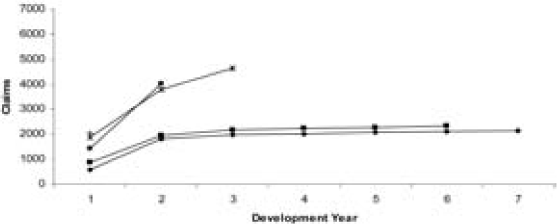
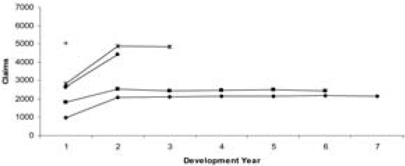
Tables 1 and 2 show the data. In order to illustrate the nature of the run-off of the data, Figures 1 and 2 are the plots of the data from Tables 1 and 2, respectively. From Figures 1 and 2, it can be seen that the data are stable and not excessively spread out.

The results of applying the bootstrap methodology described in this paper are shown below and are compared with the results from the straightforward chain ladder technique (noted as CL) and Mack’s method for the prediction errors. Table 3 shows that the theoretical MCL reserves (from Quarg and Mack 2004) and the mean of the bootstrap distributions, together with the chain ladder reserves when the triangles are considered separately. It can be seen that the bootstrap means are close to the theoretical values, for both the paid and incurred claims.

Table 4 displays the bootstrap prediction error of the MCL reserves projected by both paid and incurred claims. Also shown are the prediction errors for the Mack method. It can be seen that the MCL prediction errors are lower than those of the Mack method.

Since the purpose of the MCL method is to use more data to improve the estimation of the reserves, it is expected that the prediction errors should be lower than the Mack model. This is confirmed for these data by Table 5, which shows that the prediction error, as a percentage of the reserve, is lower for the MCL reserves than the prediction error of the reserves from the Mack model.

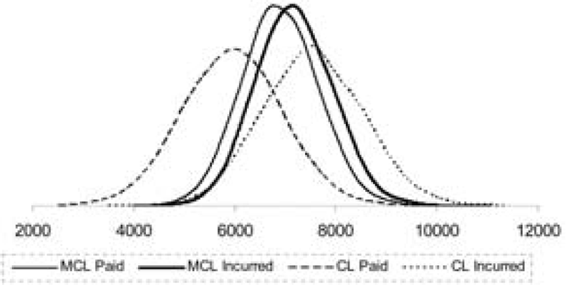
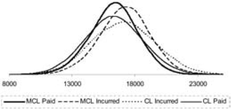
In Figure 3, the distributions of the MCL and CL reserve projections for paid and incurred claims are plotted. Figure 3 shows that the paid and incurred best reserve estimates are very close when using the MCL approach. In contrast, the paid and incurred best reserve estimates projected by the chain ladder method are much further apart. Furthermore, the CL method provides a much more spread-out distribution than the MCL approach, in the case of both paid and incurred claims.

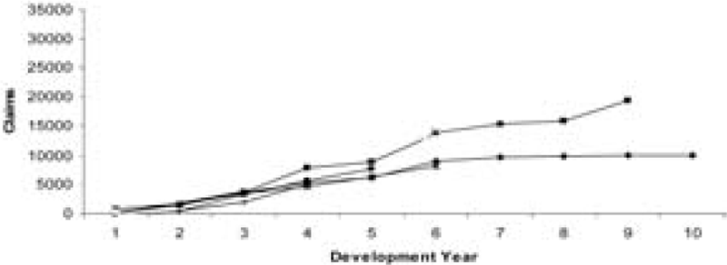
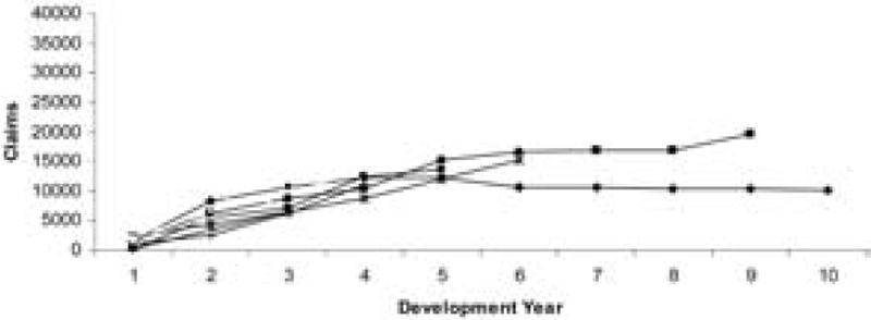
Example 2. In this section, a set of aggregate data from Lloyd’s syndicates is considered. In this case, the data are not as stable or well behaved and the results are quite different. Tables 6 and 7 show the data, which are plotted in Figures 4 and 5. It can be seen from these figures that the data are much more unstable and more spread out compared with the previous two examples.

The MCL method still produces consistent ultimate loss predictions for this data set, as shown in Table 8. However, the prediction error contained in Table 9, estimated by the bootstrap MCL approach, appears not to offer such an improvement as was seen in Example 1.

Table 10 shows a comparison of the prediction errors as a percentage of the reserve, and again it can be seen that the results do not indicate that the MCL method is a significant improvement over the CL model. The conclusion from this is that although the MCL method uses more data, and should be expected to produce lower prediction errors, this is not always the case in practice. We believe that the reason for this is that the assumptions made by the MCL method—the specific dependencies assumed—are not as strong as expected in this case. A conclusion from this is that the data have to be examined carefully before the MCL method is applied.

This conclusion is reinforced by Figure 6, which shows the predictive distributions.

6. Conclusion

This paper has shown how a bootstrapping approach can be used to estimate the predictive distribution of outstanding claims for the MCL model. The model deals with two dependent data sets, the paid and incurred claims triangles, for general insurance reserving purposes. We believe that bootstrapping is well suited for these purposes from a practical point of view, since it avoids complicated theoretical calculations and is easily implemented in a simple spreadsheet. This paper adapts the method by taking account of the dependence observed in the data and resampling pairwise.

A number of examples have been given, which show that the MCL model does not always produce superior results to the straightforward CL model. As a consequence, we believe that it is important for the data to be carefully checked to test whether the dependency assumptions of the MCL model are valid for each data set before it is applied.

---

Acknowledgment

Funding for this project from Lloyd’s of London is gratefully acknowledged.