1. Introduction
Since the late 1980s actuarial science has been moving gradually from methods to models. The movement was made possible by personal computers; it was made necessary by insurance competition. Actuaries, who used to be known for fitting curves and extrapolating from data, are now likely to be fitting models and explaining data.
Statistical modeling seeks to explain a block of observed data as a function of known variables. The model makes it possible to predict what will be observed from new instances of those variables. However, rarely, if ever, does the function perfectly explain the data. A successful model, as well as seeming reasonable, should explain the observations tolerably well. So the deterministic model y = f(X) gives way to the approximation y ≈ f(X), which is restored to equality with the addition of a random error term: y = f(X) + e. The simplest model is the homoskedastic linear statistical model (LSM) with vector form y = Xβ + e, in which E[e] = 0 and Var[e] = σ2I. According to LSM theory, β̂ = (X′X)–1X′y is the best linear unbiased estimator (BLUE) of β, even if the elements of error vector e are not normally distributed.
The fact that the errors resultant in most actuarial models are not normally distributed raises two questions. First, does non-normality in the randomness affect the accuracy of a model’s predictions? The answer is “Yes, sometimes seriously.” Second, can models be made “robust,” i.e., able to deal properly with non-normal error? Again, “Yes.” Three attempts to do so are 1} to relax parts of BLUE, especially linearity and unbiasedness (robust estimation), 2} to incorporate explicit distributions into models (GLM), and 3} to bootstrap. Bootstrapping a linear model begins with solving it conventionally. One obtains β̂ and the expected observation vector ŷ = Xβ̂. Gleaning information from the residual vector ê = y − ŷ, one can simulate proper, or more realistic, “pseudo-error” vectors ei* and pseudo-observations yi = ŷ + ei*. Iterating the model over the yi will produce pseudo-estimates β̂i and pseudo-predictions in keeping with the apparent distribution of error. Of the three attempts, bootstrapping is the most commonsensical.
The errors resultant in most actuarial models are not normally distributed.
Our purpose herein is to introduce a distribution for non-normal error that is suited to bootstrapping in general, but especially as regards the asymmetric and skewed data that actuaries regularly need to model. As useful candidates for non-normal error, Sections 2 and 3 will introduce the log-gamma random variable and its linear combinations. Section 4 will settle on a linear combination that arguably maximizes the ratio of versatility to complexity, the generalized logistic random variable. Section 5 will examine its special cases. Finally, Section 6 will estimate by maximum likelihood the parameters of one such distribution from actual data. The most mathematical and theoretical subjects are relegated to Appendices A–C.
2. The log-gamma random variable
If X ∼ Gamma(α, θ), then Y = ln X is a random variable whose support is the entire real line. Hence, the logarithm converts a one-tailed distribution into a two-tailed. Although a leftward shift of X would move probability onto the negative real line, such a left tail would be finite. The logarithm is a natural way, even the natural way, to transform one infinite tail into two infinite tails. Because the logarithm function strictly increases, the probability density function of Y ∼ Log-Gamma(α, θ) is:
\[
\begin{aligned}
f_{Y}(u) & =f_{X=e^{Y}}\left(e^{u}\right) \frac{d e^{u}}{d u}=\frac{1}{\Gamma(\alpha)} e^{-\frac{e^{u}}{\theta}}\left(\frac{e^{u}}{\theta}\right)^{\alpha-1} \frac{1}{\theta} e^{u} \\
& =\frac{1}{\Gamma(\alpha)} e^{-\frac{e^{u}}{\theta}}\left(\frac{e^{u}}{\theta}\right)^{\alpha}
\end{aligned}
\]
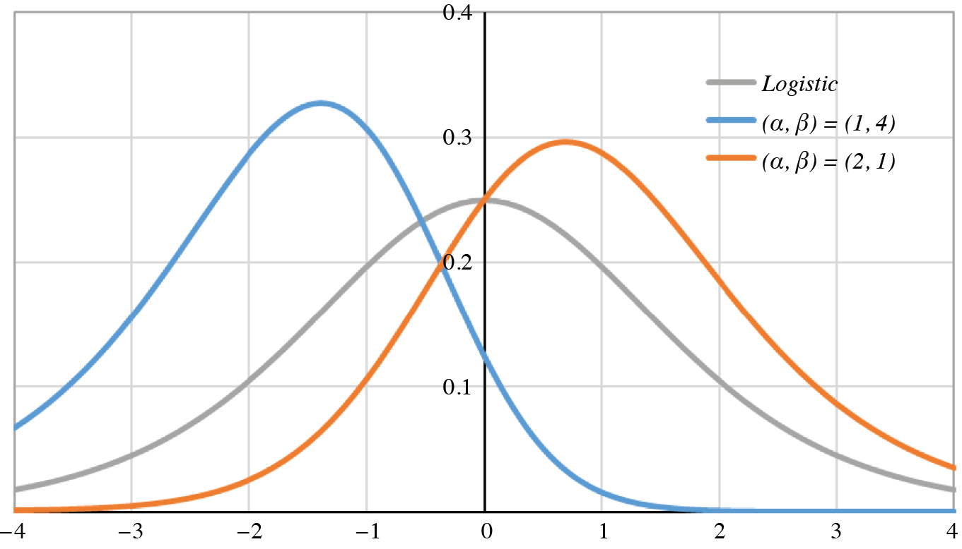
Figure 1 contains a graph of the probability density functions of both X and Y = ln X for X ∼ Gamma(1, 1) ∼ Exponential(1). The log-gamma tails are obviously infinite, and the curve itself is skewed to the left (negative skewness).
The log-gamma moments can be derived from its moment generating function:
\[
M_{Y}(t)=E\left[e^{t Y}\right]=E\left[e^{t \ln X}\right]=E\left[X^{t}\right]=\frac{\Gamma(\alpha+t)}{\Gamma(\alpha)} \theta^{t}
\]
Even better is to switch from moments to cumulants by way of the cumulant generating function:
\[
\begin{array}{l}
\psi_{Y}(t)=\ln M_{Y}(t)=\ln \Gamma(\alpha+t)-\ln \Gamma(\alpha)+t \ln \theta \\
\psi_{Y}(0)=\ln M_{Y}(0)=0
\end{array}
\]
The cumulants (κn) are the derivatives of this function evaluated at zero, the first four of which are:
\[
\begin{array}{c}
\psi_{Y}^{\prime}(t)=\psi(\alpha+t)+\ln \theta \\
\kappa_{1}=E[Y]=\psi_{Y}^{\prime}(0)=\psi(\alpha)+\ln \theta \\
\psi_{Y}^{\prime \prime}(t)=\psi^{\prime}(\alpha+t) \\
\kappa_{2}=\operatorname{Var}[Y]=\psi_{Y}^{\prime \prime}(0)=\psi^{\prime}(\alpha)>0 \\
\psi_{Y}^{\prime \prime \prime}(t)=\psi^{\prime \prime}(\alpha+t) \\
\kappa_{3}=\operatorname{Skew}[Y]=\psi_{Y}^{\prime \prime \prime}(0)=\psi^{\prime \prime}(\alpha)<0 \\
\psi_{Y}^{\mathrm{iv}}(t)=\psi^{\prime \prime \prime}(\alpha+t) \\
\kappa_{4}=\operatorname{XsKurt}[Y]=\psi_{Y}^{\mathrm{iv}}(0)=\psi^{\prime \prime \prime}(\alpha)>0
\end{array}
\]
The scale factor θ affects only the mean. The alternating inequalities of κ2, κ3, and κ4 derive from the polygamma formulas of Appendix A.3. The variance, of course, must be positive; the negative skewness confirms the appearance of the log-gamma density in Figure 1. The positive excess kurtosis means that the log-gamma distribution is “platykurtic;” its kurtosis is more positive than that of the normal distribution.
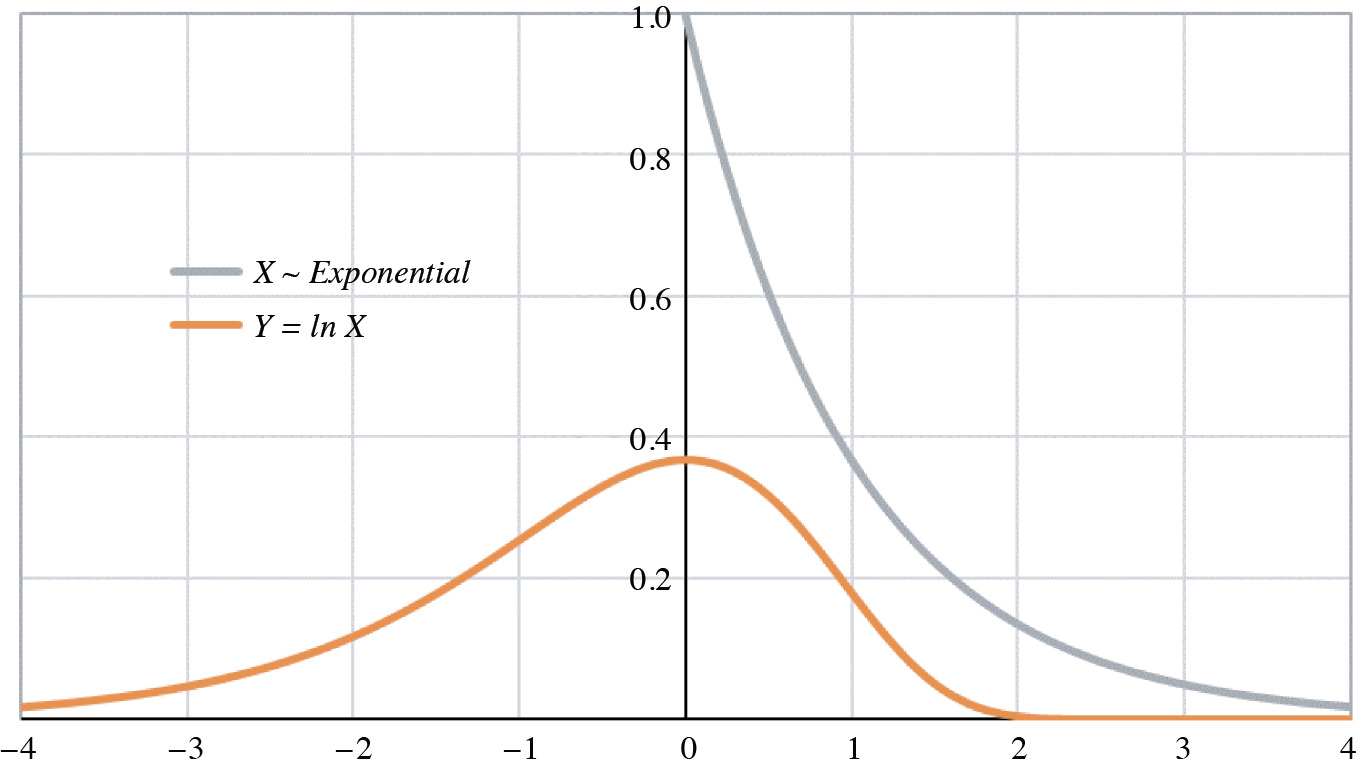
Figure 1.Probability densities
Since the logarithm is a concave downward function, it follows from Jensen’s inequality:
\[
\begin{array}{c}
E[Y=\ln X] \leq \ln E[X] \\
\psi(\alpha)+\ln \theta \leq \ln (\alpha \theta)=\ln (\alpha)+\ln (\theta) \\
\psi(\alpha) \leq \ln (\alpha)
\end{array}
\]
Because the probability is not amassed, the inequality is strict: ψ(α) < ln(α) for α > 0. However, when E[X] = αθ is fixed at unity and as α → ∞, the variance of X approaches zero. Hence, \(\lim _{\alpha \rightarrow \infty}\) (ln(α) – ψ(α)) = ln 1 = 0. It is not difficult to prove that \(\lim _{\alpha \rightarrow 0^{+}}\) (ln(α) – ψ(α)) = ∞, as well as that ln(α) − ψ(α) strictly decreases. Therefore, for every y > 0 there exists exactly one α > 0 for which y = ln(α) – ψ(α).
The log-gamma random variable becomes an error term when its expectation equals zero. This requires the parameters to satisfy the equation E[Y] = ψ(α) + ln θ = 0, or θ = e−ψ(α). Hence, the simplest of all log-gamma error distributions is Y ∼ Log-Gamma (α, e−ψ(α)) = ln(X ∼ Gamma(α, e−ψ(α))).
3. Weighted sums of log-gamma random variables
Multiplying the log-gamma random variable by negative one reflects its distribution about the y-axis. This does not affect the even moments or cumulants; but it reverses the signs of the odd ones. For example, the skewness of –Y = −ln X = ln X−1 is positive.
Now let Y be a γ-weighted sum of independent log-gamma random variables Yk, which resolves into a product of powers of independent gamma random variables Xk ∼ Gamma(αk, θk):
\[
Y=\sum_{k} \gamma_{k} Y_{k}=\sum_{k} \gamma_{k} \ln X_{k}=\sum_{k} \ln X_{k}^{\gamma_{k}}=\ln \prod_{k} X_{k}^{\gamma_{k}}
\]
Although the Xk must be independent of one another, their parameters need not be identical. Because of the independence:
\[
\begin{aligned}
\psi_{Y}(t) & =\ln E\left[e^{t Y}\right]=\ln E\left[e^{t \sum_{k} \gamma_{k} Y}\right]=\ln E\left[\prod_{k} e^{t \gamma_{k} Y_{k}}\right] \\
& =\ln \prod_{k} E\left[e^{t \gamma_{k} Y_{k}}\right]=\sum_{k} \ln E\left[e^{t \gamma_{k} Y_{k}}\right]=\sum_{k} \psi_{Y_{k}}\left(t \gamma_{k}\right)
\end{aligned}
\]
The nth cumulant of the weighted sum is:
\[
\begin{aligned}
\kappa_{n}(Y) & =\left.\frac{d^{n} \psi_{Y}(t)}{d t^{n}}\right|_{t=0}=\left.\frac{d^{n}}{d t^{n}} \sum_{k} \psi_{Y_{k}}\left(t \gamma_{k}\right)\right|_{t=0} \\
& =\left.\sum_{k} \frac{d^{n} \psi_{Y_{k}}\left(t \gamma_{k}\right)}{d t^{n}}\right|_{t=0}=\sum_{k} \gamma_{k}^{n} \psi_{Y_{k}}^{[n]}(0) \\
& =\sum_{k} \gamma_{k}^{n} \kappa_{n}\left(Y_{k}\right)
\end{aligned}
\]
So the nth cumulant of a weighted sum of independent random variables is the weighted sum of the cumulants of the random variables, the weights being raised to the nth power.
Using the cumulant formulas from the previous section, we have:
\[
\begin{aligned}
\kappa_{1}(Y) & =\sum_{k} \gamma_{k} \kappa_{1}\left(Y_{k}\right)=\sum_{k} \gamma_{k} \psi\left(\alpha_{k}\right)+\sum_{k} \gamma_{k} \ln \left(\theta_{k}\right) \\
& =\sum_{k} \gamma_{k} \psi\left(\alpha_{k}\right)+C \\
\kappa_{2}(Y) & =\sum_{k} \gamma_{k}^{2} \kappa_{2}\left(Y_{k}\right)=\sum_{k} \gamma_{k}^{2} \psi^{\prime}\left(\alpha_{k}\right) \\
\kappa_{3}(Y) & =\sum_{k} \gamma_{k}^{3} \kappa_{3}\left(Y_{k}\right)=\sum_{k} \gamma_{k}^{3} \psi^{\prime \prime}\left(\alpha_{k}\right) \\
\kappa_{4}(Y) & =\sum_{k} \gamma_{k}^{4} \kappa_{4}\left(Y_{k}\right)=\sum_{k} \gamma_{k}^{4} \psi^{\prime \prime \prime}\left(\alpha_{k}\right)
\end{aligned}
\]
In general, κm+1 (Y) = \(\sum_{k}\)γkm+1ψ[m](αk) + IF(m = 0, C, 0). A weighted sum of n independent log-gamma random variables would provide 2n + 1 degrees of freedom for a method-of-cumulants fitting. All the scale parameters θk would be unity. As the parameter of an error distribution, C would lose its freedom, since the mean must then equal zero. Therefore, with no loss of generality, we may write \(Y=\ln \prod_k X_k^{\gamma_k}+C\) for Xk ∼ Gamma(αk, 1).
4. The generalized logistic random variable
Although any finite weighted sum is tractable, four cumulants should suffice in most practice. So let Y = γ1lnX1 + γ2lnX2 + C = \(\ln \left(X_1^{\gamma_1} X_2^{\gamma_2}\right)\) + C. Even then, one gamma should be positive and the other negative; in fact, letting one be the opposite of the other will allow Y to be symmetric in special cases. Therefore, Y = γlnX1 − γlnX2 + C = γ ln(X1/X2) + C for γ > 0 should be a useful form of intermediate complexity. Let the parameterization for this purpose be X1 ∼ Gamma (α, 1) and X2 ∼ Gamma(β, 1). Contributing to the usefulness of this form is the fact that X1/X2 is a generalized Pareto random variable, whose probability density function is:
\[
f_{X_{1} / X_{2}}(u)=\frac{\Gamma(\alpha+\beta)}{\Gamma(\alpha) \Gamma(\beta)}\left(\frac{u}{u+1}\right)^{\alpha-1}\left(\frac{1}{u+1}\right)^{\beta-1} \frac{1}{(u+1)^{2}}
\]
The not overly complicated “generalized logistic” distribution is versatile enough for modeling non-normal error.
Since eY = eC (X1/X2)γ, for –α < γt < β:
\[
\begin{aligned}
M_{Y}(t)= & E\left[e^{t Y}\right]=e^{C t} E\left[\left(X_{1} / X_{2}\right)^{\gamma t}\right] \\
= & e^{C t} \int_{u=0}^{\infty} u^{\gamma t} \frac{\Gamma(\alpha+\beta)}{\Gamma(\alpha) \Gamma(\beta)}\left(\frac{u}{u+1}\right)^{\alpha-1} \\
& \left(\frac{1}{u+1}\right)^{\beta-1} \frac{d u}{(u+1)^{2}} \\
= & e^{C t} \frac{\Gamma(\alpha+\gamma t) \Gamma(\beta-\gamma t)}{\Gamma(\alpha) \Gamma(\beta)} \int_{u=0}^{\infty} \frac{\Gamma(\alpha+\beta)}{\Gamma(\alpha+\gamma t) \Gamma(\beta-\gamma t)} \\
& \left(\frac{u}{u+1}\right)^{\alpha+\gamma t-1}\left(\frac{1}{u+1}\right)^{\beta-\gamma t-1} \frac{d u}{(u+1)^{2}} \\
= & e^{C t} \frac{\Gamma(\alpha+\gamma t) \Gamma(\beta-\gamma t)}{\Gamma(\alpha) \Gamma(\beta)}
\end{aligned}
\]
Hence, the cumulant generating function and its derivatives are:
\[
\begin{aligned}
\psi_{Y}(t)= & \ln M_{Y}(t)=C t+\ln \Gamma(\alpha+\gamma t) \\
& -\ln \Gamma(\alpha)+\ln \Gamma(\beta-\gamma t)-\ln \Gamma(\beta) \\
\psi_{Y}^{\prime}(t)= & \gamma(\psi(\alpha+\gamma t)-\psi(\beta-\gamma t))+C \\
\psi_{Y}^{\prime \prime}(t)= & \gamma^{2}\left(\psi^{\prime}(\alpha+\gamma t)+\psi^{\prime}(\beta-\gamma t)\right)
\end{aligned}
\]
\[
\begin{array}{l}
\psi_{Y}^{\prime \prime \prime}(t)=\gamma^{3}\left(\psi^{\prime \prime}(\alpha+\gamma t)-\psi^{\prime \prime}(\beta-\gamma t)\right) \\
\psi_{Y}^{\mathrm{iv}}(t)=\gamma^{4}\left(\psi^{\prime \prime \prime}(\alpha+\gamma t)+\psi^{\prime \prime \prime}(\beta-\gamma t)\right)
\end{array}
\]
And so, the cumulants are:
\[
\begin{array}{l}
\kappa_{1}=E[Y]=\psi_{Y}^{\prime}(0)=C+\gamma(\psi(\alpha)-\gamma(\beta)) \\
\kappa_{2}=\operatorname{Var}[Y]=\psi_{Y}^{\prime \prime}(0)=\gamma^{2}\left(\psi^{\prime}(\alpha)+\psi^{\prime}(\beta)\right)>0 \\
\kappa_{3}=\operatorname{Skew}[Y]=\psi_{Y}^{\prime \prime \prime}(0)=\gamma^{3}\left(\psi^{\prime \prime}(\alpha)-\psi^{\prime \prime}(\beta)\right) \\
\kappa_{4}=\operatorname{XsKurt}[Y]=\psi_{Y}^{\mathrm{iv}}(0)=\gamma^{4}\left(\psi^{\prime \prime \prime}(\alpha)+\psi^{\prime \prime \prime}(\beta)\right)>0
\end{array}
\]
The three parameters α, β, γ could be fitted to empirical cumulants κ2, κ3, and κ4. For an error distribution C would equal γ(ψ(β) – ψ(α)). Since κ4 > 0, the random variable Y is platykurtic.
Since Y = γ ln(X1/X2) + C, Z = (Y − C)/γ = ln(X1/X2) may be considered a reduced form. From the generalized Pareto density above, we can derive the density of Z:
\[
\begin{aligned}
f_{Z}(u) & =f_{X_{1} / X_{2}=e^{Z}}\left(e^{u}\right) \frac{d e^{u}}{d u} \\
& =\frac{\Gamma(\alpha+\beta)}{\Gamma(\alpha) \Gamma(\beta)}\left(\frac{e^{u}}{e^{u}+1}\right)^{\alpha-1}\left(\frac{1}{e^{u}+1}\right)^{\beta-1} \frac{1}{\left(e^{u}+1\right)^{2}} \cdot e^{u} \\
& =\frac{\Gamma(\alpha+\beta)}{\Gamma(\alpha) \Gamma(\beta)}\left(\frac{e^{u}}{e^{u}+1}\right)^{\alpha}\left(\frac{1}{e^{u}+1}\right)^{\beta}
\end{aligned}
\]
Z ∼ ln(Gamma(α, 1)/Gamma(β, 1)) is a “generalized logistic” random variable (Wikipedia [Generalized logistic distribution]).
The probability density functions of generalized logistic random variables are skew-symmetric:
\[
\begin{aligned}
f_{\frac{1}{Z}=\ln \frac{X_{2}}{X_{1}}}(-u) & =\frac{\Gamma(\beta+\alpha)}{\Gamma(\beta) \Gamma(\alpha)}\left(\frac{e^{-u}}{e^{-u}+1}\right)^{\beta}\left(\frac{1}{e^{-u}+1}\right)^{\alpha} \\
& =\frac{\Gamma(\alpha+\beta)}{\Gamma(\alpha) \Gamma(\beta)}\left(\frac{e^{u}}{e^{u}+1}\right)^{\alpha}\left(\frac{1}{e^{u}+1}\right)^{\beta} \\
& =f_{Z=\ln \frac{X_{1}}{X_{2}}}(u)
\end{aligned}
\]
In Figure 2 are graphed three generalized logistic probability density functions.

Figure 2.Generalized logistic densities
The density is symmetric if and only if α = β; the gray curve is that of the logistic density, for which α = β = 1. The mode of the generalized-logistic (α, β) density is umode = ln α/β. Therefore, the mode is positive [or negative] if and only if α > β [or α < β]. Since the digamma and tetragamma functions ψ, ψ″ strictly increase over the positive reals, the signs of E[Z] = ψ(α) – ψ(β) and Skew[Z] = ψ″ (α) – ψ″(β) are the same as the sign of α − β. The positive mode of the orange curve (2, 1) implies positive mean and skewness, whereas for the blue curve (1, 4) they are negative.
5. Special cases
Although the probability density function of the generalized logistic random variable is of closed form, the form of its cumulative distribution function is not closed, save for the special cases of α = 1 and β = 1. The special case of α = 1 reduces X1/X2 to an ordinary Pareto. In this case, the cumulative distribution is \(F_{Z}(u)=1-\left(\frac{1}{e^{u}+1}\right)^{\beta}\). Likewise, the special case of β = 1 reduces X1/X2 to an inverse Pareto. In that case, \(F_{Z}(u)=\left(\frac{e^{u}}{e^{u}+1}\right)^{\alpha}\). It would be easy to simulate values of Z in both cases by the inversion method (Klugman, Panjer, and Wilmot [1998, Appendix H.2]).
Quite interesting is the special case α = β. For Z is symmetric about its mean if and only if α = β, in which case all the odd cumulants higher than the mean equal zero. Therefore, in this case:
\[
f_{Z}(u)=\frac{\Gamma(2 \alpha)}{\Gamma(\alpha)^{2}} \frac{\left(e^{u}\right)^{\alpha}}{\left(e^{u}+1\right)^{2 \alpha}}
\]
Symmetry is confirmed in as much as fZ(−u) = fZ(u). When α = β = 1, \(f_{Z}(u)=\frac{e^{u}}{\left(e^{u}+1\right)^{2}}\), whose cumulative distribution is \(F_{Z}(u)=\frac{e^{u}}{e^{u}+1}=\left(\frac{e^{u}}{e^{u}+1}\right)^{\alpha=1}=\) \(1-\left(\frac{1}{e^{u}+1}\right)^{\beta=1}\). In this case, Z is a logistic distribution. Its mean and skewness are zero. As for its even cumulants:
\[
\begin{aligned}
\kappa_{2} & =\operatorname{Var}[Z]=\psi^{\prime}(\alpha)+\psi^{\prime}(\beta)=2 \psi^{\prime}(1) \\
& =2 \sum_{k=1}^{\infty} \frac{1}{k^{2}}=2 \cdot \zeta(2)=2 \frac{\pi^{2}}{6}=\frac{\pi^{2}}{3} \approx 3.290 \\
\kappa_{4} & =\operatorname{XsKurt}[Z]=\psi^{\prime \prime \prime}(\alpha)+\psi^{\prime \prime \prime}(\beta)=2 \psi^{\prime \prime \prime}(1) \\
& =2 \cdot 6 \sum_{k=1}^{\infty} \frac{1}{k^{4}}=12 \cdot \zeta(4)=12 \cdot \frac{\pi^{4}}{90}=\frac{2 \pi^{4}}{15} \approx 12.988
\end{aligned}
\]
Instructive also is the special case α = β = ½. Since Γ(½) = \(\sqrt{\pi}\) , the probability density function in this case is \(f_{Z}(x)=\frac{1}{\pi} \frac{e^{x / 2}}{e^{x}+1}\). The constant \(\frac{1}{\pi}\) suggests a connection with the Cauchy density \(\frac{1}{\pi} \frac{1}{u^{2}+1}\) (Wikepedia [Cauchy distribution]). Indeed, the density function of the random variable W = eZ/2 is:
\[
\begin{aligned}
f_{W}(u) & =f_{Z=2 \ln W}(2 \ln u) \frac{d(2 \ln u)}{d u} \\
& =\frac{1}{\pi} \frac{u}{u^{2}+1} \frac{2}{u}=\frac{2}{\pi} \frac{1}{u^{2}+1}
\end{aligned}
\]
This is the density function of the absolute value of the standard Cauchy random variable.
6. A maximum-likelihood example
Table 1 shows 85 standardized error terms from an additive-incurred model. A triangle of incremental losses by accident-year row and evaluation-year column was modeled from the exposures of its 13 accident years. Variance by column was assumed to be proportional to exposure. A complete triangle would have \(\sum_{k=1}^{13} k=91\) observations, but we happened to exclude six.
Table 1.Ordered error sample (85 = 17 \(\times\) 5)
| −2.287 |
−0.585 |
−0.326 |
−0.009 |
0.658 |
| −1.575 |
−0.582 |
−0.317 |
0.009 |
0.663 |
| −1.428 |
−0.581 |
−0.311 |
0.010 |
0.698 |
| −1.034 |
−0.545 |
−0.298 |
0.012 |
0.707 |
| −1.022 |
−0.544 |
−0.267 |
0.017 |
0.821 |
| −1.011 |
−0.514 |
−0.260 |
0.019 |
0.998 |
| −0.913 |
−0.503 |
−0.214 |
0.038 |
1.009 |
| −0.879 |
−0.501 |
−0.202 |
0.090 |
1.061 |
| −0.875 |
−0.487 |
−0.172 |
0.095 |
1.227 |
| −0.856 |
−0.486 |
−0.167 |
0.123 |
1.559 |
| −0.794 |
−0.453 |
−0.165 |
0.222 |
1.966 |
| −0.771 |
−0.435 |
−0.162 |
0.255 |
1.973 |
| −0.726 |
−0.429 |
−0.115 |
0.362 |
2.119 |
| −0.708 |
−0.417 |
−0.053 |
0.367 |
2.390 |
| −0.670 |
−0.410 |
−0.050 |
0.417 |
2.414 |
| −0.622 |
−0.384 |
−0.042 |
0.417 |
2.422 |
| −0.612 |
−0.381 |
−0.038 |
0.488 |
2.618 |
The sample mean is nearly zero at 0.001. Three of the five columns are negative, and the positive errors are more dispersed than the negative. Therefore, this sample is positively skewed, or skewed to the right. Other sample cumulants are 0.850 (variance), 1.029 (skewness), and 1.444 (excess kurtosis). The coefficients of skewness and of kurtosis are 1.314 and 1.999.
By maximum likelihood we wished to explain the sample as coming from Y = γZ + C, where Z = ln(X1/X2) ∼ ln(Gamma(α, 1)/Gamma(β, 1)), the generalized logistic variable of Section 4 with distribution:
\[
f_{Z}(u)=\frac{\Gamma(\alpha+\beta)}{\Gamma(\alpha) \Gamma(\beta)}\left(\frac{e^{u}}{e^{u}+1}\right)^{\alpha}\left(\frac{1}{e^{u}+1}\right)^{\beta}
\]
So, defining z(u; C, γ) = (u − C)/γ, whereby z(Y) = Z, we have the distribution of Y:
\[
\begin{aligned}
f_{Y}(u) & =f_{Z=z(Y)}(z(u)) z^{\prime}(u) \\
& =\frac{\Gamma(\alpha+\beta)}{\Gamma(\alpha) \Gamma(\beta)}\left(\frac{e^{z(u)}}{e^{z(u)}+1}\right)^{\alpha}\left(\frac{1}{e^{z(u)}+1}\right)^{\beta} \frac{1}{\gamma}
\end{aligned}
\]
The logarithm, or the log-likelihood, is:
\[
\begin{aligned}
\ln f_{Y}(u)= & \ln \Gamma(\alpha+\beta)-\ln \Gamma(\alpha)-\ln \Gamma(\beta) \\
& +\alpha z(u)-(\alpha+\beta) \ln \left(e^{z(u)}+1\right)-\ln \gamma
\end{aligned}
\]
This is a function in four parameters; C and γ are implicit in z(u). With all four parameters free, the likelihood of the sample could be maximized. Yet it is both reasonable and economical to estimate Y as a “standard-error” distribution, i.e., as having zero mean and unit variance. In Excel it sufficed us to let the Solver add-in maximize the log-likelihood with respect to α and β, giving due consideration that C and γ, constrained by zero mean and unit variance, are themselves functions of α and β. As derived in Section 4, E[Y] = C + γ(ψ(α) – ψ(β)) and Var[Y] = γ2(ψ′(α) + ψ′(β)). Hence, standardization requires that \(\gamma(\alpha, \beta)=1 / \sqrt{\psi^{\prime}(\alpha)+\psi^{\prime}(\beta)}\) and that C(α, β) = γ(α, β) · (ψ(β) – ψ(α)). The log-likelihood maximized at α̂ = 0.326 and β̂ = 0.135. Numerical derivatives of the GAMMALN function approximated the digamma and trigamma functions at these values. The remaining parameters for a standardized distribution must be Ĉ = −0.561 and γ̂ = 0.122. Figure 3 graphs the maximum-likelihood result.
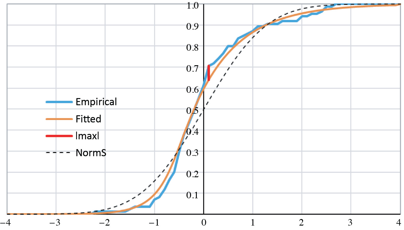
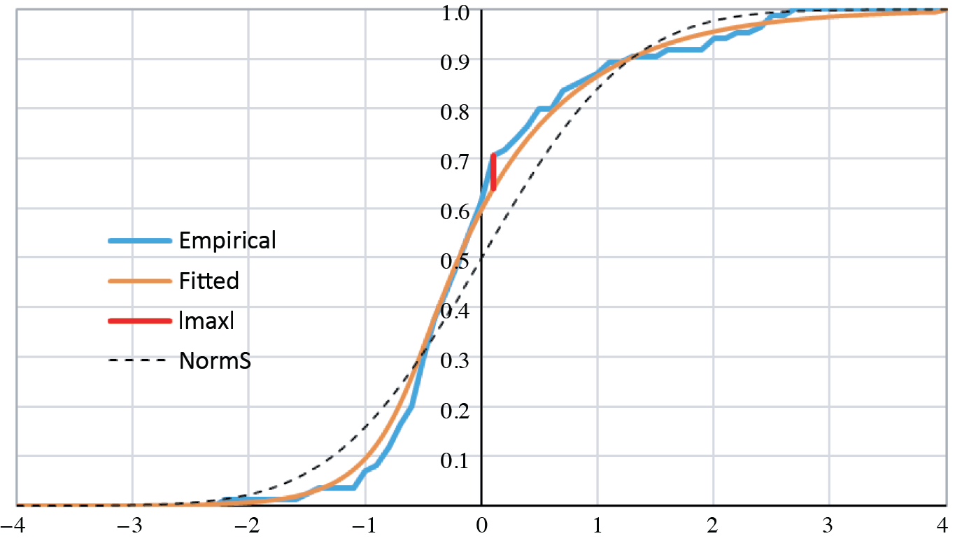
Figure 3.Empirical and fitted CDFs
The maximum absolute difference between the empirical and the fitted, |max| = 0.066, occurs at x = 0.1. We tested its significance with a “KS-like” (Kolmogorov-Smirnov, cf. Hogg and Klugman [1984, p. 104]) statistic. We simulated 1,000 samples of 85 instances from the fitted distribution, i.e., from the Y distribution with its four estimated parameters. Each simulation provided an empirical cumulative distribution, whose maximum absolute deviation we derived from the fitted distribution over the interval [−4, 4] in steps of 0.1. Figure 4 contains the graph of the cumulative density function of |max|.
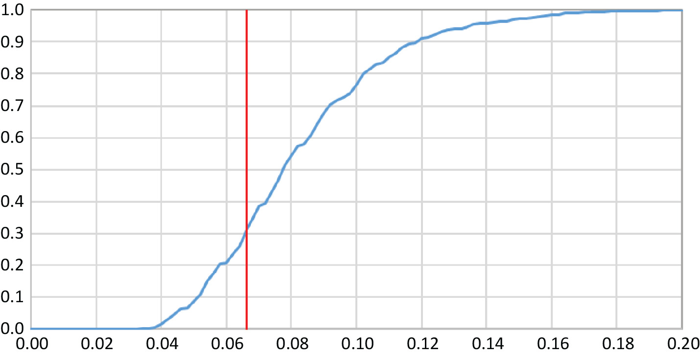
Figure 4.Distributon of |max|
The actual deviation of 0.066 coincides with the 31st percentile, or about with the lower tercile. The dashed line in Figure 3 (legend “NormS”) represents the cumulative standard-normal distribution. The empirical distribution has more probability below zero and a heavier right tail. Simulations with these logistic error terms are bound to be more accurate than simulations defaulted to normal errors.
7. Conclusion
Actuaries are well schooled in loss distributions, which are non-negative, positively skewed, and right-tailed. The key to a versatile distribution of error is to combine logarithms of loss distributions. Because most loss distributions are transformations of the gamma distribution, the log-gamma distribution covers most of the possible combinations. The generalized logistic distribution strikes a balance between versatility and complexity. It should be a recourse to the actuary seeking to bootstrap a model whose residuals are not normally distributed.
Appendices
Appendix A. The gamma, log-gamma, and polygamma functions
A.1. The gamma function as an integral
The modern form of the gamma function is Γ(α) = \(\int_{x=0}^{\infty}\) e−xxα−1dx. The change of variable t = e−x (or x = −ln t = ln 1/t) transforms it into:
\[
\Gamma(\alpha)=\int_{t=1}^{0} t\left(\ln \frac{1}{t}\right)^{\alpha-1}\left(-\frac{d t}{t}\right)=\int_{t=0}^{1}\left(\ln \frac{1}{t}\right)^{\alpha-1} d t
\]
According to Havil [2003, p. 53], Leonhard Euler used the latter form in his pioneering work during 1729–1730. It was not until 1809 that Legendre named it the gamma function and denoted it with the letter ‘Γ’. The function records the struggle between the exponential function e−x and the power function xα−1, in which the former ultimately prevails and forces the convergence of the integral for α > 0.
Of course, \(\Gamma(1)=\int_{x=0}^{\infty} e^{-x} d x=1\). The well-known recurrence formula Γ(α + 1) = αΓ(α) follows from integration by parts:
\[
\begin{aligned}
\alpha \Gamma(\alpha) & =\alpha \int_{x=0}^{\infty} e^{-x} x^{\alpha-1} d x=\int_{x=0}^{\infty} e^{-x} d\left(x^{\alpha}\right)=\left.e^{-x} x^{\alpha}\right|_{0} ^{\infty} \\
& -\int_{x=0}^{\infty} x^{\alpha} d\left(e^{-x}\right)=0+\int_{x=0}^{\infty} e^{-x} x^{\alpha+1-1} d x=\Gamma(\alpha+1)
\end{aligned}
\]
It is well to note that in order for e−xxα|0∞ to equal zero, α must be positive. For positive-integral values of α, Γ(α) = (α − 1)!; so the gamma function extends the factorial to the positive real numbers. In this domain the function is continuous, even differentiable, as well as positive. Although \(\lim _{\alpha \rightarrow 0^{+}} \Gamma(\alpha)=\infty\), \(\lim _{\alpha \rightarrow 0^{+}} \alpha \Gamma(\alpha)=\lim _{\alpha \rightarrow 0} \Gamma(\alpha+1)=\Gamma(1)=1\). So \(\Gamma(\alpha) \sim \frac{1}{\alpha}\) as α → 0+. As α increases away from zero, the function decreases to a minimum of approximately Γ(1.462) = 0.886, beyond which it increases. So, over the positive real numbers the gamma function is ‘U’ shaped, or concave upward.
The simple algebra \(1=\frac{\Gamma(\alpha)}{\Gamma(\alpha)}=\frac{\int_{x=0}^{\infty} e^{-x} x^{\alpha-1} d x}{\Gamma(\alpha)}=\) \(\int_{x=0}^{\infty} \frac{1}{\Gamma(\alpha)} e^{-x} x^{\alpha-1} d x\) indicates that \(f(x)=\frac{1}{\Gamma(\alpha)} e^{-x} x^{\alpha-1}\) is the probability density function of what we will call a Gamma(α, 1)-distributed random variable, or simply Gamma(α)-distributed with θ = 1 understood. For k > −α, the kth moment of X ∼ Gamma(α) is:
\[
\begin{aligned}
E\left[X^{k}\right] & =\int_{x=0}^{\infty} x^{k} \frac{1}{\Gamma(\alpha)} e^{-x} x^{\alpha-1} d x \\
& =\frac{\Gamma(\alpha+k)}{\Gamma(\alpha)} \int_{x=0}^{\infty} \frac{1}{\Gamma(\alpha+k)} e^{-x} x^{\alpha+k-1} d x \\
& =\frac{\Gamma(\alpha+k)}{\Gamma(\alpha)}
\end{aligned}
\]
Therefore, for k = 1 and 2, E[X] = α and E[X2] = α(α + 1). Hence, Var[X] = α.
A.2. The gamma function as an infinite product
Euler found that the gamma function could be expressed as the infinite product:
\[
\Gamma(x)=\lim _{n \rightarrow \infty} \frac{n!n^{x}}{x(1+x) \ldots(n+x)}
\]
\[
=\lim _{n \rightarrow \infty} \frac{n^{x}}{x\left(1+\frac{x}{1}\right) \ldots\left(1+\frac{x}{n}\right)}
\]
As a check, \(\Gamma(1)=\lim _{n \rightarrow \infty} \frac{n!n}{(n+1)!}=\lim _{n \rightarrow \infty} \frac{n}{n+1}=1\). Moreover, the recurrence formula is satisfied:
\[
\begin{aligned}
\Gamma(x+1)= & \lim _{n \rightarrow \infty} \frac{n!n^{x+1}}{(1+x) \ldots(n+x)(n+1+x)} \\
= & x \lim _{n \rightarrow \infty} \frac{n!n^{x}}{x(1+x) \ldots(n+x)} \\
& \lim _{n \rightarrow \infty} \frac{n}{(n+1+x)}=x \Gamma(x)
\end{aligned}
\]
Hence, by induction, the integral and infinite-product definitions are equivalent for positive-integral values of x. It is the purpose of this section to extend the equivalence to all positive real numbers.
The proof is easier in logarithms. The log-gamma function is \(\ln \Gamma(\alpha)=\ln \int_{x=0}^{\infty} e^{-x} x^{\alpha-1} d x\). The form of its recursive formula is lnΓ(α + 1) = ln(αΓ(α)) = lnΓ(α) + ln α. Its first derivative is:
\[
\begin{aligned}
(\ln \circ \Gamma)^{\prime}(\alpha) & =\frac{d}{d \alpha} \ln \Gamma(\alpha) \equiv \frac{\Gamma^{\prime}(\alpha)}{\Gamma(\alpha)} \\
& =\frac{\int_{x=0}^{\infty} e^{-x} x^{\alpha-1} \ln x d x}{\Gamma(\alpha)} \\
& =\int_{x=0}^{\infty} \frac{1}{\Gamma(\alpha)} e^{-x} x^{\alpha-1} \ln x d x=E[Y]
\end{aligned}
\]
So the first derivative of lnΓ(α) is the expectation of Y ∼ Log-Gamma(α), as defined in Section 2. The second derivative is:
\[
\begin{aligned}
(\ln \circ \Gamma)^{\prime \prime}(\alpha) & =\frac{d}{d \alpha} \frac{\Gamma^{\prime}(\alpha)}{\Gamma(\alpha)} \\
& =\frac{\Gamma(\alpha) \Gamma^{\prime \prime}(\alpha)-\Gamma^{\prime}(\alpha) \Gamma^{\prime}(\alpha)}{\Gamma(\alpha) \Gamma(\alpha)}
\end{aligned}
\]
\[
\begin{array}{l}
=\frac{\Gamma^{\prime \prime}(\alpha)}{\Gamma(\alpha)}-\left(\frac{\Gamma^{\prime}(\alpha)}{\Gamma(\alpha)}\right)^{2} \\
=\int_{x=0}^{\infty} \frac{1}{\Gamma(\alpha)} e^{-x} x^{\alpha-1}(\ln x)^{2} d x-E[Y]^{2} \\
=E\left[Y^{2}\right]-E[Y]^{2}=\operatorname{Var}[Y]>0
\end{array}
\]
Because the second derivative is positive, the log-gamma function is concave upward over the positive real numbers.
Now let n ∈ {2, 3, . . .} and x ∈ (0, 1]. So 0 < n − 1 < n < n + x ≤ n + 1. We consider the slope of the log-gamma secants over the intervals [n – 1, n], [n, n + x], and [n, n + 1]. Due to the upward concavity, the order of these slopes must be:
\[
\begin{array}{c}
\frac{\ln \Gamma(n)-\ln \Gamma(n-1)}{n-(n-1)}<\frac{\ln \Gamma(n+x)-\ln \Gamma(n)}{(n+x)-n} \\
\leq \frac{\ln \Gamma(n+1)-\ln \Gamma(n)}{(n+1)-n}
\end{array}
\]
Using the recurrence formula and multiplying by positive x, we continue:
\[
\begin{array}{c}
x \ln (n-1)<\ln \Gamma(n+x)-\ln \Gamma(n) \leq x \ln (n) \\
x \ln (n-1)+\ln \Gamma(n)<\ln \Gamma(n+x) \leq x \ln (n)+\ln \Gamma(n)
\end{array}
\]
But lnΓ(n) = \(\sum_{k=1}^{n-1} \ln k\) and ln Γ(n + x) = lnΓ(x) + ln x +
\(\sum_{k=1}^{n-1} \ln (k+x)\). Hence:
\[
\begin{aligned}
\begin{aligned}
x & \ln (n-1)+\sum_{k=1}^{n-1} \ln k \\
& <
\end{aligned} & \ln \Gamma(x)+\ln x \\
& \quad+\sum_{k=1}^{n-1} \ln (k+x) \leq x \ln (n)+\sum_{k=1}^{n-1} \ln k \\
x \ln (n-1)+\sum_{k=1}^{n-1} \ln k & -\ln x-\sum_{k=1}^{n-1} \ln (k+x)<\ln \Gamma(x) \\
& \leq x \ln (n)+\sum_{k=1}^{n-1} \ln k-\ln x-\sum_{k=1}^{n-1} \ln (k+x)
\end{aligned}
\]
\[
\begin{aligned}
x \ln (n-1)-\ln x-\sum_{k=1}^{n-1} & \ln \left(1+\frac{x}{k}\right)<\ln \Gamma(x) \\
& \leq x \ln (n)-\ln x-\sum_{k=1}^{n-1} \ln \left(1+\frac{x}{k}\right)
\end{aligned}
\]
This string of inequalities, in the middle of which is ln Γ(x), is true for n ∈{2, 3, . . .}. As n approaches infinity, \(\lim _{n \rightarrow \infty}\)[x ln(n) – x ln(n − 1)] \(=x \lim _{n \rightarrow \infty} \ln \left(\frac{n}{n-1}\right)\) = \(x \ln \left(\lim _{n \rightarrow \infty} \frac{n}{n-1}\right)\) = xln1 = 0. So lnΓ(x) is sandwiched between two series that have the same limit. Hence:
\[
\begin{aligned}
\ln \Gamma(x) & =-\ln x+\lim _{n \rightarrow \infty}\left\{x \ln (n-1)-\sum_{k=1}^{n-1} \ln \left(1+\frac{x}{k}\right)\right\} \\
& =-\ln x+\lim _{n \rightarrow \infty}\left\{x \ln (n)-\sum_{k=1}^{n} \ln \left(1+\frac{x}{k}\right)\right\}
\end{aligned}
\]
If the limit did not converge, then lnΓ(x) would not converge. Nevertheless, Appendix C constructs a proof of the limit’s convergence. But for now we can finish this section by exponentiation:
\[
\begin{aligned}
\Gamma(x) & =e^{\ln \Gamma(x)} \\
& =\frac{1}{x} e^{\lim _{n \rightarrow \infty}\left\{x \ln (n)-\sum_{k=1}^{n} \ln \left(1+\frac{x}{k}\right)\right\}} \\
& =\frac{1}{x} \lim _{n \rightarrow \infty}\left\{e^{x \ln (n)-\sum_{k=1}^{n} \ln \left(1+\frac{x}{k}\right)}\right\} \\
& =\frac{1}{x} \lim _{n \rightarrow \infty} \frac{n^{x}}{\prod_{k=1}^{n}\left(1+\frac{x}{k}\right)} \\
& =\lim _{n \rightarrow \infty} \frac{n^{x}}{x\left(1+\frac{x}{1}\right) \ldots\left(1+\frac{x}{n}\right)}
\end{aligned}
\]
The infinite-product form converges for all complex numbers z ∉ {0, −1, −2, . . .}; it provides the analytic continuation to the integral form. With the infinite-product form, Havil [2003, pp. 58f] easily derives the complement formula Γ(x)Γ(1 − x) = π/sin(πx). Consequently, Γ(½)Γ(½) = π/sin(π/2) = π.
A.3. Derivatives of the log-gamma function
The derivative of the gamma function is Γ′(a) = \(\frac{d}{d \alpha} \int_{x=0}^{\infty} e^{-x} x^{\alpha-1} d x=\int_{x=0}^{\infty} e^{-x} \frac{d\left(x^{\alpha-1}\right)}{d \alpha} d x=\int_{x=0}^{\infty} e^{-x} x^{\alpha-1} \ln x d x\)
So, for X ∼ Gamma(α):
\[
\begin{aligned}
E[\ln X] & =\int_{x=0}^{\infty} \ln x \frac{1}{\Gamma(\alpha)} e^{-x} x^{\alpha-1} d x \\
& =\frac{1}{\Gamma(\alpha)} \int_{x=0}^{\infty} e^{-x} x^{\alpha-1} \ln x d x \\
& =\frac{\Gamma^{\prime}(\alpha)}{\Gamma(\alpha)}=\frac{d}{d \alpha} \ln \Gamma(\alpha)
\end{aligned}
\]
Because the derivative of ln Γ(α) has proven useful, mathematicians have named it the “digamma” function: \(\psi(\alpha)=\frac{d}{d \alpha} \ln \Gamma(\alpha)\). Therefore, E[ln X] = ψ(α). Its derivatives are the trigamma, tetragamma, and so on. Unfortunately, Excel does not provide these functions, although one can approximate them from GAMMALN by numerical differentiation. The R and SAS programming languages have the trigamma function but stop at the second derivative of ln Γ(α). The remainder of this appendix deals with the derivatives of the log-gamma function.
According to the previous section:
\[
\ln \Gamma(x)=-\ln x+\lim _{n \rightarrow \infty}\left\{x \ln (n)-\sum_{k=1}^{n} \ln \left(1+\frac{x}{k}\right)\right\}
\]
Hence the digamma function is:
\[
\begin{aligned}
\psi(x) & =\frac{d}{d x} \ln \Gamma(x)=-\frac{1}{x}+\lim _{n \rightarrow \infty}\left\{\ln n-\sum_{k=1}^{n} \frac{1}{k+x}\right\} \\
& =\lim _{n \rightarrow \infty}\left\{\ln n-\sum_{k=0}^{n} \frac{1}{k+x}\right\}
\end{aligned}
\]
Its recurrence formula is:
\[
\begin{aligned}
\psi(x+1) & =\lim _{n \rightarrow \infty}\left\{\ln n-\sum_{k=0}^{n} \frac{1}{k+1+x}\right\} \\
& =\lim _{n \rightarrow \infty}\left\{\ln n-\sum_{k=0}^{n} \frac{1}{k+x}\right\}+\frac{1}{0+x}=\psi(x)+\frac{1}{x}
\end{aligned}
\]
Also, \(\psi(1)=\lim _{n \rightarrow \infty}\left\{\ln n-\sum_{k=0}^{n} \frac{1}{k+1}\right\}=\lim _{n \rightarrow \infty}\) \(\left\{\ln n-\sum_{k=1}^{n+1} \frac{1}{k}\right\}=-\lim _{n \rightarrow \infty}\left\{\sum_{k=1}^{n} \frac{1}{k}-\ln n\right\}=-\gamma\). Euler was
the first to see that \(\lim _{n \rightarrow \infty}\left\{\sum_{k=1}^{n} \frac{1}{k}-\ln n\right\}\) converged. He named it ‘C’ and estimated its value as 0.577218. Eventually it was called the Euler-Mascheroni constant γ, whose value to six places is really 0.577216.
The successive derivatives of the digamma function are:
\[
\begin{aligned}
\psi^{\prime}(x) & =\frac{d}{d x} \lim _{n \rightarrow \infty}\left\{\ln n-\sum_{k=0}^{n} \frac{1}{k+x}\right\}=\sum_{k=0}^{\infty} \frac{1}{(k+x)^{2}} \\
\psi^{\prime \prime}(x) & =-2 \sum_{k=0}^{\infty} \frac{1}{(k+x)^{3}} \\
\psi^{\prime \prime \prime}(x) & =6 \sum_{k=0}^{\infty} \frac{1}{(k+x)^{4}}
\end{aligned}
\]
The general formula for the nth derivative is ψ[n](x) = (−1)n−1n!\(\sum_{k=0}^{\infty} \frac{1}{(k+x)^{n+1}}\) with recurrence formula:
\[
\begin{aligned}
\psi^{[n]}(x+1) & =(-1)^{n-1} n!\sum_{k=0}^{\infty} \frac{1}{(k+1+x)^{n+1}} \\
& =(-1)^{n-1} n!\sum_{k=0}^{\infty} \frac{1}{(k+x)^{n+1}}-\frac{(-1)^{n-1} n!}{x^{n+1}} \\
& =\psi^{[n]}(x)+\frac{(-1)^{n} n!}{x^{n+1}}
\end{aligned}
\]
Finally, ψ[n](1) = (−1)n−1n!\(\sum_{k=0}^{\infty} \frac{1}{(k+1)^{n+1}}=(-1)^{n-1}\) \(n!\sum_{k=1}^{\infty} \frac{1}{k^{n+1}}=(-1)^{n-1} n!\zeta(n+1)\). A graph of the digamma through pentagamma functions appears in Wikipedia [Polygamma function].
Appendix B. Moments versus cumulants
Actuaries and statisticians are well aware of the moment generating function (mgf) of random variable \(X\):
\[
M_X(t)=E\left[e^{t X}\right]=\int_X e^{t x} f(x) d x
\]
Obviously, \(M_X(0)=E[1]=1\). It is called the mgf because its derivatives at zero, if convergent, equal the (non-central) moments of \(X\), i.e.:
\[
\begin{aligned}
M_X^{[n]}(0) & =\left.\frac{d^n}{d t^n} E\left[e^{t X}\right]\right|_{t=0}=E\left[\left.\frac{d^n e^{t X}}{d t^n}\right|_{t=0}\right] \\
& =E\left[X^n e^{0 \cdot X}\right]=E\left[X^n\right] .
\end{aligned}
\]
The mgf for the normal random variable is \(M_{N\left(\mu, \sigma^2\right)}(t)=e^{\mu t+\sigma^2 t^2 / 2}\). The mgf of a sum of independent random variables equals the product of their mgfs:
\[
\begin{aligned}
M_{X+Y}(t) & =E\left[e^{t(X+Y)}\right]=E\left[e^{t X} e^{t Y}\right] \\
& =E\left[e^{t X}\right] E\left[e^{t Y}\right]=M_X(t) M_Y(t)
\end{aligned}
\]
The cumulant generating function (cgf) of \(X\), or \(\psi_X(t)\) is the natural logarithm of the moment generating function. So \(\psi_X(0)=0\); and for independent summands:
\[
\begin{aligned}
\psi_{X+Y}(t) & =\ln M_{X+Y}(t)=\ln M_X(t) M_Y(t) \\
& =\ln M_X(t)+\ln M_Y(t)=\psi_X(t)+\psi_Y(t)
\end{aligned}
\]
The \(n\)th cumulant of \(X\), or \(\kappa_n(X)\), is the \(n\)th derivative of the cgf evaluated at zero. The first two cumulants are identical to the mean and the variance:
\[
\begin{aligned}
\kappa_1(X)= & \left.\frac{d \ln M_X(t)}{d t}\right|_{t=0}=\left.\frac{M_X^{\prime}(t)}{M_X(t)}\right|_{t=0}=E[X] \\
\kappa_2(X) & =\left.\frac{d}{d t} \frac{M_X^{\prime}(t)}{M_X(t)}\right|_{t=0}=\left.\frac{-M_X^{\prime}(t) M_X^{\prime \prime}(t)}{M_X^2(t)}\right|_{t=0} ^{\prime}(t) \\
= & E\left[X^2\right]-E[X] E[X]=\operatorname{Var}[X]
\end{aligned}
\]
One who performs the somewhat tedious third derivative will find that the third cumulant is identical to the skewness. So the first three cumulants are equal to the first three central moments. This amounts to a proof that the first three central moments are additive.
However, the fourth and higher cumulants do not equal their corresponding central moments. In fact, defining the central moments as \(\mu_n=E\left[(X-\mu)^n\right]\), the next three cumulant relations are:
\[
\begin{aligned}
& \kappa_4=\mu_4-3 \mu_2^2=\mu_4-3 \sigma^4 \\
& \kappa_5=\mu_5-10 \mu_2 \mu_3 \\
& \kappa_6=\mu_6-15 \mu_2 \mu_4-10 \mu_3^2+30 \mu_2^3
\end{aligned}
\]
The cgf of a normal random variable is \(\psi_{N\left(\mu, \sigma^2\right)}(t)= \ln e^{\mu t+\sigma^2 t / 2}=\mu t+\sigma^2 t^2 / 2\). It first two cumulants equal \(\mu\) and \(\sigma^2\), and its higher cumulants are zero. Therefore, the third and higher cumulants are relative to the zero values of the corresponding normal cumulants. So third and higher cumulants could be called “excess of the normal,” although this in practice is done only for the fourth cumulant. Because \(\mu_4=E\left[(X-\mu)^4\right]\) is often called the kurtosis, ambiguity is resolved by calling \(\kappa_4\) the “excess kurtosis,” or the kurtosis in excess of \(\mu_4=E\left[N\left(0, \sigma^2\right)^4\right]=E\left[N(0,1)^4\right] \cdot \sigma^4=3 \sigma^4\).
Appendix C. Log-gamma convergence
In Appendix A. 2 we proved that for real \(\alpha>0\) :
\[
\begin{aligned}
\ln \left(\int_{x=0}^{\infty} e^{-x} x^{\alpha-1} d x\right)= & \ln \Gamma(\alpha)=-\ln \alpha \\
& +\lim _{n \rightarrow \infty}\left\{\alpha \ln n-\sum_{k=1}^n \ln \left(1+\frac{\alpha}{k}\right)\right\}
\end{aligned}
\]
There we argued that the “real-ness” of the left side for all \(\alpha>0\) implies the convergence of the limit on the right side; otherwise, the equality would be limited or qualified. Nevertheless, it is valuable to examine the convergence of the log-gamma limit, as we will now do.
Define \(a_n(x)=\frac{x}{n}-\ln \left(1+\frac{x}{n}\right)\) for natural number \(n\) and real number \(x\). To avoid logarithms of negative numbers, \(x>-1\), or \(x \in(-1, \infty)\). The root of this group of functions is \(f(x)=x-\ln (1+x)\). Since the two functions \(y=x\) and \(y=\ln (1+x)\) are tangent to each other at \(x=0\), \(f(0)=f^{\prime}(0)=0\). Otherwise, the line is above the logarithm and \(f(x \neq 0)>0\). Since \(f^{\prime \prime}(x)=1 /(1+x)^2\) must be positive, \(f(x)\) is concave upward with a global minimum over \((-1, \infty)\) at \(x=0\).
For now, let us investigate the convergence of \(\varphi(x)=\sum_{n=1}^{\infty} a_n(x)=\sum_{n=1}^{\infty}\left\{\frac{x}{n}-\ln \left(1+\frac{x}{n}\right)\right\}\). Obviously, \(\varphi(x=0)=0\). But if \(x \neq 0\), for some \(\xi \in(\min (n, n+x)\), \(\max (n, n+x)\) ):
\[
\begin{aligned}
a_n(x) & =\frac{x}{n}-\ln \left(1+\frac{x}{n}\right) \\
& =\frac{x}{n}-\ln \left(\frac{n+x}{n}\right) \\
& =\frac{x}{n}-\int_{u=n}^{n+x} \frac{d u}{u} \\
& =\frac{x}{n}-((n+x)-n) \frac{1}{\xi} \\
& =\frac{x}{n}-\frac{x}{\xi} \\
& =x\left(\frac{1}{n}-\frac{1}{\xi}\right)
\end{aligned}
\]
Regardless of the sign of \(x\) :
\[
|x|\left|\left(\frac{1}{n}-\frac{1}{n}\right)\right|<\left|a_n(x)\right|<|x|\left|\left(\frac{1}{n}-\frac{1}{n+x}\right)\right|
\]
The lower bound reduces to zero; the upper to \(|x|\left|\frac{x}{n(n+x)}\right|=\frac{|x|^2}{|n||n+x|}=\frac{x^2}{n|n+x|}\). But \(n+x\) must be positive, since \(x>-1\). Therefore, for \(x \neq 0\) :
\[
0<\left|a_n(x)\right|<\frac{x^2}{n(n+x)}
\]
For \(x=0\), equality prevails. And so for all \(x>-1\) :
\[
0 \leq\left|a_n(x)\right| \leq \frac{x^2}{n(n+x)}
\]
Now absolute convergence, or the convergence of \(\sum_{n=1}^{\infty}\left|a_n(x)\right|\), is stricter than simple convergence. If \(\sum_{n=1}^{\infty}\left|a_n(x)\right|\) converges, then so too does \(\varphi(x)=\) \(\sum_{n=1}^{\infty} a_n(x)\). And \(\sum_{n=1}^{\infty}\left|a_n(x)\right|\) converges, if it is bounded from above. The following string of inequalities establishes the upper bound:
\[
\begin{aligned}
\sum_{n=1}^{\infty}\left|a_n(x)\right| & \leq \sum_{n=1}^{\infty} \frac{x^2}{n(n+x)} \\
& \leq \frac{x^2}{1(1+x)}+\sum_{n=2}^{\infty} \frac{x^2}{n(n+x)} \\
& \leq \frac{x^2}{1+x}+x^2 \sum_{n=2}^{\infty} \frac{x^2}{n(n+x)} \\
& \leq \frac{x^2}{1+x}+x^2 \sum_{n=2}^{\infty} \frac{1}{(n-1)^2} \\
& \leq \frac{x^2}{1+x}+x^2\left(\frac{\pi^2}{6}=\varsigma(2)=\sum_{n=1}^{\infty} \frac{1}{n^2}\right)
\end{aligned}
\]
Thus have we demonstrated the convergence of \(\varphi(x)=\sum_{n=1}^{\infty} a_n(x)=\sum_{n=1}^{\infty}\left\{\frac{x}{n}-\ln \left(1+\frac{x}{n}\right)\right\}\).
As a special case:
\[
\begin{aligned}
\lim _{n \rightarrow \infty} \sum_{k=1}^n a_k(1) & =\lim _{n \rightarrow \infty} \sum_{k=1}^n\left\{\frac{1}{k}-\ln \left(1+\frac{1}{k}\right)\right\} \\
& =\lim _{n \rightarrow \infty} \sum_{k=1}^n\left\{\frac{1}{k}-\ln \left(\frac{k+1}{k}\right)\right\} \\
& =\lim _{n \rightarrow \infty}\left\{\sum_{k=1}^n \frac{1}{k}-\ln (n+1)\right\} \\
& =\lim _{n \rightarrow \infty}\left\{\sum_{k=1}^n \frac{1}{k}-\ln (n)\right\}=\gamma \approx 0.577
\end{aligned}
\]
Returning to the limit in the log-gamma formula and replacing ’ \(\alpha\) ’ with ’ \(x\) ', we have:
\[
\begin{aligned}
& \lim _{n \rightarrow \infty}\left\{x \ln n-\sum_{k=1}^n \ln \left(1+\frac{x}{k}\right)\right\} \\
& \quad=\lim _{n \rightarrow \infty}\left\{x \ln n+\sum_{k=1}^n\left[-\frac{x}{k}+\frac{x}{k}-\ln \left(1+\frac{x}{k}\right)\right]\right\} \\
& \quad=\lim _{n \rightarrow \infty}\left\{x \ln n-\sum_{k=1}^n \frac{x}{k}\right\}+\sum_{k=1}^n\left\{\frac{x}{k}-\ln \left(1+\frac{x}{k}\right)\right\} \\
& \quad=-x \lim _{n \rightarrow \infty}\left\{\sum_{k=1}^n \frac{1}{k}-\ln (n)\right\}+\sum_{k=1}^n\left\{\frac{x}{k}-\ln \left(1+\frac{x}{k}\right)\right\} \\
& \quad=-\gamma x+\sum_{k=1}^n a_k(x)
\end{aligned}
\]
Thus, independently of the integral definition, we have proven for \(\alpha>0\) the convergence of \(\ln \Gamma(\alpha)=-\ln \alpha+\lim _{n \rightarrow \infty}\left\{\alpha \ln n-\sum_{k=1}^n \ln \left(1+\frac{\alpha}{k}\right)\right\}\).
This is but one example of a second-order convergence. To generalize, consider the convergence of \(\varphi(x)=\lim _{n \rightarrow \infty} \sum_{k=1}^n f\left(\frac{x}{k}\right)\). As with the specific \(f(x)=\) \(x-\ln (1+x)\) above, the general function \(f\) must be analytic over an open interval about zero, \(a<0<b\). Likewise, its value and first derivative at zero must be analytic over an open interval about zero, \(a<0<b\). Likewise, its value and first derivative at zero must be zero, i.e., \(f(0)=f^{\prime}(0)=0\). According to the second-order mean value theorem, for \(x \in(a, b)\), there exists a real \(\xi\) between zero and \(x\) such that:
\[
f(x)=f(0)+f^{\prime}(0) x+\frac{f^{\prime \prime}(\xi)}{2} x^2=\frac{f^{\prime \prime}(\xi)}{2} x^2
\]
Therefore, there exist \(\xi_k\) between zero and \(\frac{x}{k}\) such that \(\varphi(x)=\lim _{n \rightarrow \infty} \sum_{k=1}^n f\left(\frac{x}{k}\right)=\lim _{n \rightarrow \infty} \sum_{k=1}^n \frac{f^{\prime \prime}\left(\xi_k\right)}{2}\left(\frac{x}{k}\right)^2\).
Again, we appeal to absolute convergence. If \(\lim _{n \rightarrow \infty} \sum_{k=1}^n\left|\frac{f^{\prime \prime}\left(\xi_k\right)}{2}\left(\frac{x}{k}\right)^2\right|=\frac{x^2}{2} \lim _{n \rightarrow \infty} \sum_{k=1}^n \frac{\left|f^{\prime \prime}\left(\xi_k\right)\right|}{k^2}\) converges, then \(\varphi(x)\) converges. But every \(\xi_k\) belongs to the closed interval \(\Xi\) between 0 and \(x\). And since \(f\) is analytic over \((a, b) \supset \Xi, f^{\prime \prime}\) is continuous over \(\Xi\). Since a continuous function over a closed interval is bounded, \(0 \leq\left|f^{\prime \prime}\left(\xi_k\right)\right| \leq M\) for some real \(M\). So, at length:
\[
\begin{aligned}
0 \leq \lim _{n \rightarrow \infty} \sum_{k=1}^n \frac{\left|f^{\prime \prime}\left(\xi_k\right)\right|}{k^2} \leq \lim _{n \rightarrow \infty} \sum_{k=1}^n \frac{M}{k^2} & =M \lim _{n \rightarrow \infty} \sum_{k=1}^n \frac{1}{k^2} \\
& =M \zeta(2)=M \frac{\pi^2}{6}
\end{aligned}
\]
Consequently, \(\lim _{n \rightarrow \infty} \sum_{k=1}^n f\left(\frac{x}{k}\right)\) converges to a real number for every function \(f\) that is analytic over some domain about zero and for which \(f(0)=f^{\prime}(0)=0\). The convergence must be at least of the second order; a first-order convergence would involve \(\lim _{n \rightarrow \infty} \sum_{k=1}^n \frac{M}{k}\) and the divergence of the harmonic series.
The same holds true for analytic functions over complex domains. Another potentially important secondorder convergence is \(\varphi(z)=\lim _{n \rightarrow \infty} \sum_{k=1}^n\left\{e^{\frac{z}{k}}-\left(1+\frac{z}{k}\right)\right\}\).