Capital Allocation by Percentile Layer

undefined

1. Required capital, required rate of return, and capital allocation

How much capital should an insurance firm hold? And what rate of return must the firm achieve on this capital? While these questions are of critical importance to the firm, external forces in the operating environment often dictate the answers. For example, regulators and rating agencies greatly influence the amount of capital the firm must hold; in addition, investors influence both the amount of capital the firm holds and the required rate of return on this capital. Therefore, the issues of the amount of capital and the required rate of return on capital are often ultimately beyond the decision-making power of the company; rather, they are demands that the operating environment imposes upon the firm.

Given that a firm must hold a certain amount of capital, the firm essentially incurs a firm-wide overhead cost related to the required rate of return on this capital. Management often desires to allocate this cost, like other overhead costs, to subsets of the firm such as subsidiaries, business units, and product lines. How should the firm allocate the cost of required return on capital? This is the question of capital allocation.

1.1. Why is capital allocation important?

How a firm allocates capital, similar to other cost allocation decisions, can significantly affect the measured profitability of a particular line of business. Moreover, allocating capital can affect target pricing margins and the volume of business the company writes in each line of business and product type. As a result, the topic is critically important and often the subject of contentious debate among the heads of the firm’s various business units.

1.2. Defining the scope of the problem

We will restrict our discussion to the situation of a publicly traded insurance company that writes property catastrophe business, both insurance and reinsurance, covering several perils around the world; we will exclude long-tail casualty business in an attempt to simplify our discussion to a single-year time horizon problem. We will assume that investors require that the firm holds total capital based upon the Value at Risk (VaR) at the 99th percentile and that the required return can be expressed as an annual percentage rate of return on this amount of capital. We will only address the issue of allocating total capital.

1.3. Allocating capital to those who “cause” the firm to hold capital

Mango (2003) has stressed that the entire capital of the firm is available to pay the claim of any single policy. Thus, the required rate of return on capital is a cost that accrues on the total firm level, and Kreps (2005) has clarified that capital allocation is really the allocation of the required rate of return on capital. Mango (1998) also has highlighted the connection between allocating capital and broader issues of cost allocation.^[1] Therefore, similar to other cost allocation situations, we want to connect the firmwide cost of capital to those subsets of the firm that require, cause, or spur the company to incur this cost: essentially, to match the expenditure to its source.^[2] In other words, we desire to allocate the cost of capital to those business units, products, perils, reinsurance contracts, and individual insurance policies that contribute to the loss scenarios that cause the firm to hold capital.^[3] However, identifying the loss scenarios that are the true reason for or cause of holding capital can be confusing; in the case of holding capital based upon VaR, one approach that can help clarify which loss scenarios cause the firm to hold capital is to investigate which loss scenarios use capital.

1.4. So who causes the firm to hold capital? Who uses capital?

In our situation, the company must hold capital based upon Value at Risk (VaR) at the 99th percentile. Therefore, one seemingly attractive approach for allocating capital is to use VaR (99%) as a basis (or risk measure) for allocation. Under this approach, the company allocates capital to components of the firm based upon their contributions to the total firm’s VaR (99%) loss scenario. In fact, this approach is so attractive that it has already been discussed as a possible basis for allocation (among several other candidates) by Kreps (2005) and Venter (2006). One key characteristic of this approach is that it allocates capital only to those components that contribute to one particular loss scenario (e.g., the 99th percentile loss) but not to scenarios that are either greater than or less than the selected VaR percentile.^[4]

Similarly, one might suggest using Tail Value at Risk (TVaR) as a basis for allocating capital. According to this view, one allocates capital to a line of business only to the extent of its contribution to loss events greater than or equal to the 99th percentile loss (or other selected threshold). Again, loss scenarios that are less than the TVaR threshold percentile receive no capital allocation.

Intuitively, however, this characterization of using VaR (and TVaR) to allocate capital seems unsatisfying; to clarify what is bothersome, we will use a thought experiment with simplified numbers.

1.5. Thought experiment #1

Assume we are dealing with two perils:

1. Wind: 20% chance of 99M loss, else zero

2. Earthquake (EQ): 5% chance of 100M loss, else zero

Assume the perils are independent. Thus, the possible scenarios for portfolio loss are:

1. 76% probability that neither peril occurs, loss = 0

2. 19% probability that only Wind occurs, loss of 99M

3. 4% probability that only EQ occurs, loss of 100M

4. 1% probability that both Wind and EQ occur, loss of 199M

Using VaR (99%) as our capital requirement, we hold 100M of capital to pay for 99% of the loss events; only the rare, 1% chance of a Wind event plus an EQ event will exceed the capital.

Many current approaches to allocation appear to have significant drawbacks.

Method #1 (“coVaR”): If we say that using VaR to set the capital requirement means that we allocate capital to the events that generate the VaR scenario of 100M, then does that mean we should only allocate capital to the EQ peril (which causes the potential loss event of 100M)—yet the Wind peril that can cause a loss event of “only” 99M receives zero capital allocation?

Method #2 (“alternative coVaR”): Another approach might be to use all events ≥ VaR to allocate. Then we allocate 80% [= 4%/(4% + 1%)] to the EQ event and 20% [= 1%/(4% + 1%)] to the “Wind+EQ” event; using Kreps’s “co-measures” approach, we can then further allocate the capital for the “Wind + EQ” event to its components:

$$\text { Wind }=49.75 \%=99 /(100+99),$$

and

$$\mathrm{EQ}=50.25 \%=100 /(100+99) .$$

In total, EQ would receive approximately 90%,

$$\mathrm{EQ}=80 \%+50.25 \% * 20 \%,$$

and

$$\begin{array}{l} \text { Wind }=49.75 \% * 20 \%\\ \text { or approximately } 10 \% \text {. } \end{array}$$

But again, the substantial possibility of a standalone Wind event of 99M has no significance?

Method #3 (“coTVaR”): Another approach might be to allocate using the TVaR measure for loss events ≥ 100M. Then the EQ event receives an allocation proportional to 80% * 100M and the Wind + EQ event receives allocation proportional to 20% * 199M. Using Kreps’s co-measures again, ultimately EQ receives 83.5% and Wind 16.5%; but again, we will allocate zero capital based upon the Only Wind event of 99M, which is much more likely to use capital and nearly as large of a loss as the EQ Only event!

The numerical example above crystallizes one of the problematic aspects of the traditional interpretation of allocating capital based upon VaR: namely, loss scenarios below the tail threshold use substantial amounts of capital, yet they receive zero capital allocation for this usage.^[5]

2. Articulating the meaning of holding capital based upon Value at Risk (VaR)

It therefore appears necessary to remind ourselves what it means for a firm to hold capital at the 99th percentile, or VaR (99%). Some common formulations state that the firm holds sufficient capital “for the 99th percentile loss,” which can lead unwittingly to the incorrect interpretation that the firm holds capital “only for the 99th percentile loss.”^[6] Indeed, the allocation approaches described above, which allocate all capital costs based only upon contribution to the VaR percentile loss scenario, are totally congruous with this interpretation. Rather, a more precise articulation of the meaning of holding VaR capital is that the firm holds sufficient capital “even for the 99th percentile loss,” but not “only for the 99th percentile loss.”

In other words, we can describe holding capital based upon VaR (99%) as follows. The firm needs to hold a certain amount of capital for small, medium, and moderately large losses; the firm also decides to hold an incremental amount of additional capital so that it can pay even for losses as large as the 99th percentile loss scenario. Therefore, according to this formulation, only an incremental portion of the firm’s capital is needed exclusively for the largest losses; a significant portion of the firm’s capital, however, serves to cover losses at lower percentiles as well.

We can also use an analogous approach to articulate the meaning of a firm holding capital based upon TVaR. Specifically, using TVaR (99%) to set capital means the firm holds capital even for the average loss scenario beyond the 99th percentile, but not only for these events.

In other words, we can describe holding capital based upon TVaR (99%) as follows. The firm needs to hold a certain amount of capital for small, medium, and moderately large losses; the firm also decides to hold an incremental amount of additional capital so that it can pay even for losses as large as the 99th percentile loss scenario. In addition, the firm also recognizes that it may sustain a loss even greater than the 99th percentile; because of this possibility, the firm holds an additional incremental amount of capital equal to the average additional loss beyond the 99th percentile. Therefore, according to this formulation, only this additional incremental amount of capital is needed exclusively for the loss scenarios that exceed the 99th percentile; a significant portion of the firm’s capital, however, serves to cover losses at lower percentiles as well.

Beyond VaR and TVaR, the same line of reasoning may be relevant when interpreting other capital benchmarks as well.

2.1. Ramifications of formulation of holding VaR capital

What are some of the ramifications of our formulation that holding capital equal to VaR (99%) means holding sufficient capital “even for a 99th percentile loss” but not “only for a 99th percentile loss”?

It would appear that we need to think about capital allocation by percentile layer. In other words, why does the firm hold capital equal to the 99th percentile loss rather than the lower amount of the 98th percentile loss? The difference between the required capital amounts at these two percentile losses can be attributed solely to those loss events that outstrip the 98th percentile. Similarly, the difference between the amount of capital at the 98th percentile loss and the 97th percentile loss can be attributed solely to those losses that exceed the 97th percentile, and so on.

Therefore, allocation of capital to loss scenarios would appear to require calculations that vary by layer of capital.

3. Defining a percentile layer of capital

Thus, we can define a percentile layer of capital as follows. Define percentile α, increment j, and percentile α + j on the interval [0, 1]. Then

$$\begin{aligned} & \text{Percentile layer of capital } (\alpha, \alpha+j)\\ & \quad = \text{Required capital at percentile } (\alpha+j)\\ & \qquad - \text{Required capital at percentile } (\alpha). \end{aligned}\tag{3.0}$$

We can also define a layer of capital as follows. Define amounts a and b, then

$$\begin{aligned} & \text{Layer of capital } (a, a+b)\\ & \quad = \text{Capital equal to amount } (a+b)\\ & \qquad - \text{Capital equal to amount } (a). \end{aligned} \tag{3.1}$$

For example, assume we have simulated 100 discrete loss events and the 78th loss (ordered from smallest to largest) is 59M and the 77th loss is 47M, then the percentile layer of capital (77%, 78%) = 59M − 47M = 12M.

3.1. Refining the percentile layer of capital

Note that we can set Capital (α) = any function of (VaR (α)). For example, if we want a 99th percentile loss to consume no more than 50% of capital, then

$$\operatorname{VaR}(99 \%)=50 \% * \text { Capital }(99 \%),$$

and

$$\operatorname{Capital}(99 \%)=2 * \operatorname{VaR}(99 \%)$$

For ease of use, we will assume that the capital required at a loss percentile will equal that loss amount:

$$\text { Capital }(\alpha)=\operatorname{VaR}(\alpha)=\text { loss percentile }(\alpha) \text {. }$$

Also, we will assume that j, which equals the width or increment of a layer’s percentiles between lower and upper bounds, equals 1/n, where n = number of available discrete values. For example, if we have 100 simulation outputs, then the layer increment j = 1%, and if we have 1000 simulated values, then j = 0.1%.

3.2. Allocating a percentile layer of capital to loss events

We can see that each layer of capital is potentially used or depleted (or “consumed” in the terminology of Mango [2003]) by loss events that exceed the lower bound of the layer, but not by loss scenarios that fall short of the lower bound of the layer (i.e., those losses that do not penetrate the layer). Thus, it is desirable to allocate each layer of capital only to those events that penetrate the layer. Another critical consideration is that some of the losses that penetrate the layer are more likely to do so than others. Therefore, each event (i) that penetrates the layer of capital receives an allocation based upon its conditional exceedance probability.

Conditional exceedance probability for event (i) = Probability of event (i) that penetrates the layer of capital/Probability of all events that penetrate the layer of capital.

Thus, for any layer of capital, we take the amount of capital (i.e., the “width” of the layer) and allocate it only to loss events that penetrate the layer. We calculate the allocation percentages based upon each loss event’s conditional probability of penetrating the layer. The allocation percentages, by definition, sum to 100% on any layer.

After performing the allocation of each layer of capital (from zero up to the required VaR capital amount, but not beyond it), we will have allocated 100% of the capital to loss events.

Many loss scenarios will penetrate several different percentile layers of capital and therefore will receive varying allocations of capital from many layers of capital. The total capital allocated to any particular loss event is simply the total, summed over all layers of capital that the loss event penetrates, of the capital allocated on each individual layer. As an example, take the 83rd percentile loss event. On each layer of capital (from zero up to the 83rd percentile layer of capital but not beyond), it receives varying amounts of allocated capital; sum across all of these layers to calculate total capital allocated to this event. Of course, each loss “event” or “scenario” may be an accumulation of losses from several business units, policies, and/or perils. But as Kreps (2005) has shown, once we have the total allocated capital for a loss scenario, we can then allocate to the subcomponents based upon their contributions to the total.

3.2.1. Applying capital allocation by percentile layer to Thought Experiment #1

In this section we will apply the procedure of capital allocation by percentile layer to the simplified numbers of Thought Experiment #1.

In Thought Experiment #1, there are four potential scenarios:

1. 76% neither peril occurs, loss = 0

2. 19% only Wind occurs, loss of 99M

3. 4% only EQ occurs, loss of 100M

4. 1% both Wind and EQ occur, loss of 199M

We hold capital equal to VaR (99%) = 100M. The layer of capital of 1M × 99M can only be penetrated (or “depleted” or “consumed”) by event #3 or #4. Event #3, the Only EQ event, has a conditional exceedance probability of 80% [4%/(4% + 1%)]. Event #4, the Wind and EQ event, has conditional exceedance probability of 20%. Therefore, we allocate the 1M in layer capital (100M − 99M) as follows:

• 80% for EQ event;

• 20% for Wind + EQ event;

• 0% for Wind only event.

The next layer of capital, 99M × 0, can be used by all 3 loss events.

• Only Wind event has conditional exceedance probability of 79% [19%/(19% + 4% + 1%)].

• Only EQ event has conditional exceedance probability of 17% [4%/(19% + 4% + 1%)].

• Wind and EQ event has conditional exceedance probability of 4% [1%/(19% + 4% + 1%)].

Therefore, the allocation of 99M in capital (99M − 0) is

• 79% for Wind;

• 17% for EQ;

• 4% for Wind + EQ.

The total capital allocation to loss event across both layers (namely, 1M × 99M and 99M × 0) is then

• Only Wind = 79% × 99M = 78.4M.

• Only EQ = 17% × 99M + 80% × 1M = 17.3M.

• Wind + EQ event = 4% × 99M + 20% × 1M = 4.3M.

The total allocated capital is 78.4 + 17.3 + 4.3 = 100 = VaR (99%).

The loss event of Wind + EQ can then be allocated further to the underlying perils that contribute to the loss event (per Kreps [2005]) as follows: In a Wind + EQ event, which receives a 4.3M allocation, Wind contributes 99M and EQ contributes 100M. Therefore, Wind % = (99/199) = 49.75%; EQ = (100/199) = 50.25%.

The total allocation to peril is therefore

• Wind = 78.4M + 49.75% × 4.3M = 80.5M, and

• EQ = 17.3M + 50.25% × 4.3M = 19.5M.

Comparing results at the 99th percentile, we see that capital allocation by percentile layer generates a significantly different allocation than a method such as coTVaR.

Allocation by percentile layer:

• Wind = 80.5%;

• EQ = 19.5%.

Allocation by coTVaR for all events ≥ 100M =

• Wind = 16.5%;

• EQ = 83.5%.

3.2.2. Thought Experiment #2

In Thought Experiment #1, capital allocation by percentile layer produced allocations that are essentially proportional to the perils’ average loss. So does this imply that the procedure will always result in such an allocation? After all, it would seem problematic to always allocate capital in proportion to the average loss; catastrophic perils with the capability to produce severe losses should receive a greater allocation of capital, regardless of the “average” outcome. Thought Experiment #2 shows that capital allocation by percentile layer will, in fact, allocate more capital to more severe perils in such a situation.

Again assume we are dealing with two perils:

1. Wind: 20% chance of 50M loss, else zero;

2. Earthquake (EQ): 5% chance of 100M loss, else zero.

Note that for Wind the average loss is 10M and for EQ the average loss is 5M.

Assume the perils are independent. Thus, the possible scenarios for portfolio loss are:

1. 76% probability that neither peril occurs, loss of 0

2. 19% probability that only Wind occurs, loss of 50M

3. 4% probability that only EQ occurs, loss of 100M

4. 1% probability that both Wind and EQ occur, loss of 150M

Using VaR (99%) as our capital requirement, we hold 100M of capital to pay for 99% of the loss events; only the rare, 1% chance of a Wind event plus an EQ event will exceed the capital. Applying capital allocation by percentile layer to the 50M × 50M layer of capital as well as the 50M × 0 layer of capital, we obtain the following allocation:

Allocation by percentile layer:

• Wind = 44%

• EQ = 56%

In contradistinction, allocation in proportion to average loss produces:

• Wind = 67%

• EQ = 33%

This example shows that capital allocation by percentile layer can produce unique allocations that are proportional neither to the average loss, nor to probability of occurrence, nor to standalone VaR.

4. Graphical description of capital allocation by percentile layer—Discrete

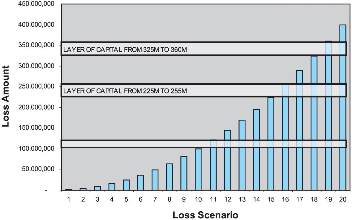
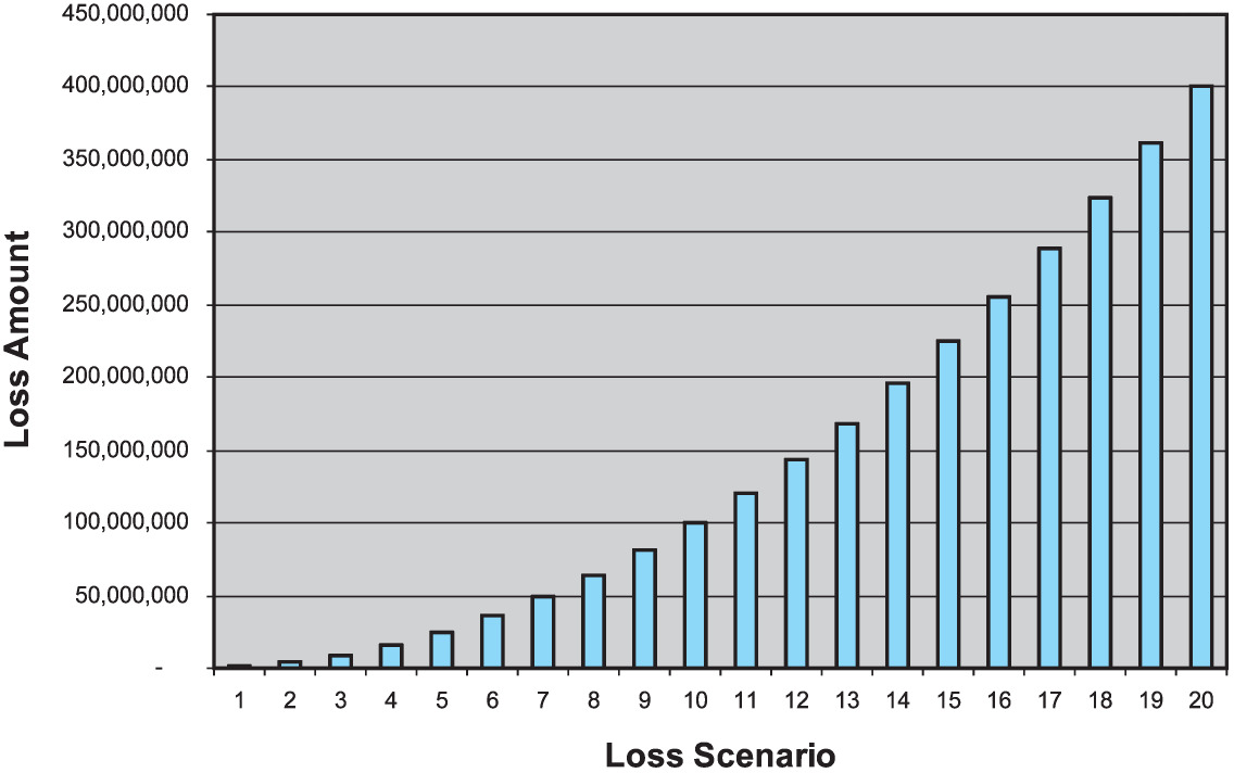
Let us view the “size of loss” distribution in graphical format to further clarify the approach; we will use sample numbers for simplicity. We will use “Lee Diagrams” (Lee 1988), namely graphs where the loss scenario number (ordered in increasing size) is plotted on the X-axis and the loss amount is plotted on the Y-axis:

In the Figure 1 example, there are 20 loss scenarios and we stipulate that the firm holds capital equal to the 19th worst loss scenario, 360M. Why is it that the firm needs to hold 360M of capital rather than just 100M of capital? It appears that loss scenarios 1 through 10, which are all less than or equal to 100M, do not require this layer of capital. In contradistinction, loss scenarios 11 through 20, which exceed 100M, clearly do utilize this layer of capital in excess of 100M. Examining in further detail, we see that all of scenarios 11 through 20 utilize the 1M layer of capital extending from 100M to 101M, but not all of them require the 1M layer of capital from 200M to 201M, and even fewer loss scenarios require the 1M layer of capital from 300M to 301M.

Thus, we must allocate each individual layer of capital to the loss events that penetrate the layer in proportion to the relative usage of the layer of capital: i.e., in proportion to the relative exceedance probability, as per Figure 2.

A numerical example:

• Loss scenario #19 is one of two events (scenarios 19 and 20) that require the 35M layer of capital from 325M to 360M.

  • Thus scenario #19 receives 1/2 allocation of this 35M of capital.

• Loss scenario #19 also is one of five events (scenarios 16 through 20) that require the firm to hold the 30M layer of capital from 225M to 255M.

  • Thus it receives 1/5 allocation of this 30M of capital.

• Apply the procedure to all layers; allocate to all loss events that exceed the lower bound of the layer via conditional exceedance probability.

Note that a loss event tends to receive a larger percentage allocation in the upper layers than in the lower layers for two reasons:

1. In the upper layers, we are allocating a full layer of capital to fewer loss events (i.e., the exceedance probability decreases as the loss amount increases); therefore, each event gets a larger share of the “overhead” of the total layer of capital.

2. In the upper layers, we are allocating a wider layer of capital because the severity of each loss event tends to outstrip the prior loss event by a greater amount (i.e., the percentile layer of capital tends to widen as the loss amount increases). This behavior will depend, however, on the particular shape of the size of loss distribution.

5. Generalization of capital allocation by percentile layer to discrete loss events

Let VaR(k) = total required capital = Σ[x(α + j) − x(α)], where

• x(α) is the loss amount at percentile α,

• j is selected percentile increment, and

• α sums from zero to (k − j).

Allocation of capital for each percentile layer of capital, across loss events:

• A Layer of Capital = [x(α + j) − x(α)].

• The allocation of the capital layer [x(α + j) − x(α)] to loss event x(i) is given by

  $$\begin{array}{l} {[x(\alpha+j)-x(\alpha)]} \\ \quad * \text { Probability }(x=x(i)) / \text { Probability }(x>x(\alpha)) . \end{array}$$

• Sum across all loss events x(i) such that i > α.

For an equivalent view, we can also look at the allocation of capital for each loss event, across all percentile layers of capital:

• A Layer of Capital = [x(α + j) − x(α)].

• The allocation of the capital layer [x(α + j) − x(α)] to loss event x(i) is given by

  $$\begin{array}{l} {[x(\alpha+j)-x(\alpha)]} \\ \quad * \text { Probability }(x=x(i)) / \text { Probability }(x>x(\alpha)) . \end{array}$$

• Sum across all layers of capital such that α ≥ 0, (α + j) ≤ min(i, k).

• Note the min(i, k) restriction. For any loss event, we sum across all layers of capital up to the amount of the given loss event, but not if the loss event exceeds the VaR threshold. In such a case, the loss beyond the VaR threshold does not generate additional allocated capital to the loss event.

6. Generalization of capital allocation by percentile layer to a continuous loss function

We can take the formulas for discrete loss events and generalize them into continuous versions.

First, we will define the inverse function of F(x), a function that accepts a percentile as input and returns the loss amount as output. Figure 3 shows a graphical depiction of this function.

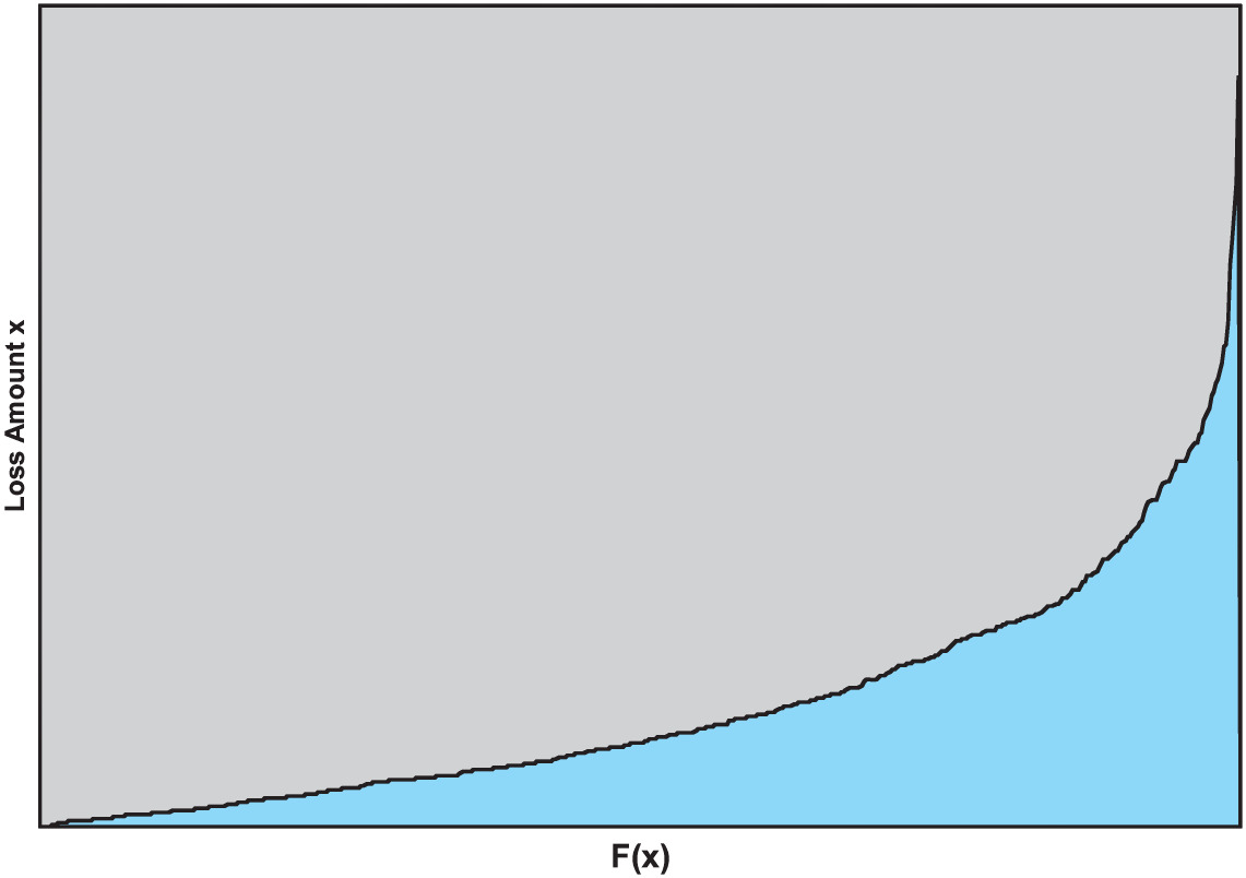
Inverse function of $F(x)$

$\qquad = F^{-1}(\alpha) = F^{-1}(F(x)) = x.$

Derivative of $F^{-1}(F(x))$

$\qquad =d F^{-1}(F(x)) / d F(x)=d x / d F(x)=1 / f(x)$.

Incremental change in loss amount

$\qquad = dx.$

Incremental change in percentile

$\qquad =dF(x).$

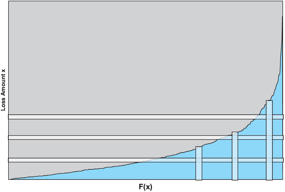
In Figure 4, each horizontal bar is a layer of capital. The horizontal length of the layer of capital, by definition, is 1.0. The infinitesimally small width of each layer of capital is dx. Each vertical bar represents a loss event, and the vertical length is the loss amount, x. The infinitesimally small width, dF(x) = f(x)dx, is the probability of the loss x.

6.1. Two alternative views of capital allocation by percentile layer

We can view the capital allocation as a “horizontal procedure” which takes each layer of capital and allocates to all loss events which penetrate the layer.

We can also view the allocation as a “vertical procedure” which takes each loss event and allocates capital to it for all layers that it penetrates.^[7]

6.2. Approach #1: Horizontal then vertical

Let x represent the loss amount and let y represent the capital.

First take an infinitesimally small layer of capital (y, y + dy) and allocate it across loss events.

Integrate across all loss events x which penetrate the layer, from x = y to x = ∞.

$$\int_{x=y}^{x=\infty} \frac{f(x)}{1-F(y)} d x \tag{6.0}$$

The allocation weights sum to 1 on each layer.

Then perform this procedure for all layers of capital:

$$\int_{y=0}^{y=\operatorname{VaR}(99 \%)} \int_{x=y}^{x=\infty} \frac{f(x)}{1-F(y)} d x d y . \tag{6.1}$$

Because capital is based upon the 99th percentile, there are no layers of capital above the 99th percentile to allocate, so we integrate y only up to VaR (99%).

The total allocated capital equals the total amount of capital, which is VaR (99%).

6.3. Approach #2: Vertical then horizontal

Let x represent the loss amount and let y represent the capital.

Each loss event uses capital on many layers of capital (y, y + dy).

Allocate to a loss event across each layer of capital:

$$\int_{y=0}^{y=x} \frac{f(x)}{1-F(y)} d y \tag{6.2}$$

Integrate y across all layers of capital less than or equal to the loss amount x.

If the loss amount x exceeds VaR (99%), we do not allocate additional layers of capital beyond VaR (99%); in such a case when x > VaR (99%), we integrate as follows:

$$\int_{y=0}^{y=\mathrm{VaR}(99 \%)} \frac{f(x)}{1-F(y)} d y \tag{6.3}$$

Then perform allocation across all loss events x:

$$\int_{x=x(0 \%)}^{x=\infty} \int_{y=0}^{y=\min (x, \operatorname{VaR}(99 \%))} \frac{f(x)}{1-F(y)} d y d x \tag{6.4}$$

6.4. Formula for allocating capital to a loss event

The “vertical view” can provide some insight into the capital allocation to each loss event.

As we saw previously (equation (6.2)), for any loss event with amount x (assuming x is below the VaR threshold and therefore the allocated capital is not capped in any way), the Allocated Capital to loss event x, AC(x), can be expressed:

$$\mathrm{AC}(x)=\int_{y=0}^{y=x} \frac{f(x)}{1-F(y)} d y . \tag{6.5}$$

Because we are integrating with respect to y, we can move f(x) outside the integral and rewrite the formula:

$$\mathrm{AC}(x)=f(x) \int_{y=0}^{y=x} \frac{1}{1-F(y)} d y \tag{6.6}$$

For completeness, also recall that if the loss event is in the tail, namely x > VaR (99%), then

$$\mathrm{AC}(x)=f(x) \int_{y=0}^{y=\mathrm{VaR}(99 \%)} \frac{1}{1-F(y)} d y \tag{6.7}$$

According to equation (6.6), the procedure of capital allocation by percentile layer says that any loss event’s allocated capital depends upon:

1. The probability of the event occurring (i.e. f(x)).

2. The severity of the loss event, or the extent to which the loss event penetrates layers of capital (i.e., the upper bound of integration is x, the loss amount).

3. The loss event’s inability to share the burden of its required capital with other loss events (i.e., ∫ 1 = [1 − F(y)]dy). We can think of this expression as a mathematical measurement of the extent to which a loss event “sticks out” or is “dissimilar in severity” to other loss events.

6.4.1. The derivative of the allocated capital to loss event

We can also use equation (6.6) to obtain the derivative of Allocated Capital to loss event with respect to the loss amount x:

$$\begin{array}{l} \frac{d}{d x}\{\mathrm{AC}(x)\} \\ \quad=\frac{d}{d x}\left\{f(x) \int_{y=0}^{y=x} \frac{1}{1-F(y)} d y\right\} \end{array} \tag{6.8}$$

$$\begin{aligned} \frac{d}{d x}\{\mathrm{AC}(x)\} & \\ = & f(x) * \frac{d}{d x}\left\{\int_{y=0}^{y=x} \frac{1}{1-F(y)} d y\right\} \\ & +\frac{d}{d x}\{f(x)\} * \int_{y=0}^{y=x} \frac{1}{1-F(y)} d y . \end{aligned} \tag{6.9}$$

Therefore,

$$\frac{d}{d x}\{\mathrm{AC}(x)\}=\frac{f(x)}{1-F(x)}+f^{\prime}(x) \int_{y=0}^{y=x} \frac{1}{1-F(y)} d y \tag{6.10}$$

We can understand formula (6.10) as saying that as the loss amount x under consideration increases, two factors simultaneously affect the loss event’s allocated capital:

1. The allocated capital increases to the extent that the loss event receives allocation from an additional layer of capital based upon conditional probability {= f(x)=[1 − F(x)]}.

2. The allocated capital changes (usually decreases) to the extent that the loss event is less likely to occur and thus receives a lower allocation on the lower layers of capital {= f′(x) ∫ 1/[1 − F(y)]dy}.

Two observations about these two factors:

1. Usually, the derivative of f(x) is negative, so item #2 is usually negative, but can be positive when the derivative of f(x) is positive.

2. When dealing with simulation output of n discrete events, each discrete event has likelihood of 1/n and thus is equally likely; therefore, the allocated capital to each larger event increases only with respect to factor #1, whereas factor #2 will equal zero.

6.4.2. Utility function

Equation (6.6) also shows how we can use capital allocation by percentile layer to describe the disutility, or “pain,” given a particular loss event x.

Let r be the required percent rate of return on capital. Then the cost of capital associated with loss event x can be written

$$r * f(x) \int_{y=0}^{y=x} \frac{1}{1-F(y)} d y \tag{6.11}$$

The cost of capital of an event, given the loss event, is then

$$r \int_{y=0}^{y=x} \frac{1}{1-F(y)} d y \tag{6.12}$$

And the total cost, given the event, equals the loss amount x plus the cost of capital:

$$x+r \int_{y=0}^{y=x} \frac{1}{1-F(y)} d y \tag{6.13}$$

Equation (6.13) shows the disutility as an additive loading to the loss amount x. Rearranging terms, we can also show the disutility as a multiplicative factor as well:

$$x\left[1+r \frac{1}{x} \int_{y=0}^{y=x} \frac{1}{1-F(y)} d y\right] \tag{6.14}$$

7. Interpretation, comments, and extensions

The procedure for capital allocation by percentile layer outlined above generates allocations that are different than many other methods, with ramifications for measuring the relative risk and profitability of various lines of business. Some methods tend to allocate the overwhelming amount of capital only to perils that contribute to the very worst scenarios; capital allocation by percentile layer, however, recognizes that when the firm holds capital even for an extremely catastrophic scenario, some of the capital also benefits other, more likely, more moderately severe downside events. On the other hand, other methods allocate capital to a broader range of loss events that consume capital, often in proportion to an average measure of downside; consequently, a severe yet unlikely event can receive the same allocation as a less severe loss that is more likely. As a numerical example, a loss event of 10% probability that consumes 10M of capital can receive the same capital allocation as a loss event of 1% probability that consumes 100M of capital. The drawback of this approach, however, is that it does not recognize that the potential extreme loss of severe events causes the firm to hold an amount of capital that far outstrips the amount required by other loss events; although the actual occurrence of one of these events is very unlikely, the cost of holding precautionary capital is quite definite. In contradistinction to these methods, capital allocation by percentile layer recognizes that severe events, despite being unlikely to occur, require the firm to hold additional capital; capital allocation by percentile layer explicitly measures this additional amount of capital and thus allocates more capital to unlikely, severe events.

7.1. Extension to TVaR

Capital allocation by percentile layer as described in this paper assumes that required capital is based upon VaR; how should we extend the procedure to apply to capital based upon TVaR? This question is addressed in further detail in Appendix B.

7.2. Additional areas of application

The application highlighted here focuses on property catastrophe risk and allocating the cost of equity capital, but the reformulation of the meaning of VaR should have similar ramifications in other areas as well.

1. Assets: Risk and capital for risky assets such as equities and fixed income securities have traditionally been defined based upon VaR metrics;^[8] as a result, methods that allocate capital among various asset classes and operating units may benefit from adopting capital allocation by percentile layer.

2. Credit portfolio modeling: According to Kalkbrener (2004), the standard approach in modeling credit portfolios uses VaR to define economic capital. However, “the allocation of portfolio VaR…is difficult”;^[9] therefore, capital allocation by percentile layer, which directly and explicitly allocates VaR capital, may be advantageous for allocating VaR capital within a credit portfolio.

3. Other forms of capital: Capital allocation by percentile layer may also be germane when the firm’s total capital does not reside in one indivisible bucket of equity capital but rather is split into different types of capital.

   a. Multiple tranches of capital: Firms often have sources of capital beyond equity capital, sometimes in the form of tranches. These tranches sustain capital depletion in a predetermined sequential order and, as a result, carry different cost of capital rates. Thus, capital allocation by percentile layer, which provides a framework for explicitly allocating various layers of capital and their costs, appears well suited for such a situation.

   b. Reinsurance: Other forms of capital that apply on a layered basis, such as excess of loss reinsurance, and their costs (i.e., the amount of risk load or margin in the reinsurance price) would also appear to be candidates for capital allocation by percentile layer.

7.3. Implementation

In many situations in which we want to implement capital allocation by percentile layer, we will be dealing with discrete output from a simulation model. By using the previously derived discrete formulas we can program a spreadsheet and achieve numerical results. Once capital amounts are allocated to each simulated loss event, we can then (per Mango, Kreps) further allocate the capital for the total loss to those individual components that contributed to the total.

7.3.1. Contributions to capital

The main focus of the analysis until now has been on the allocation of capital with respect to loss without considering premium. When measuring the allocated cost of capital for a business unit or peril or individual contract, one must also recognize that the associated premium (net of expenses) is essentially a contribution to capital or offset to allocated capital. As a result, one should subtract collected premium net of expenses from the allocated capital before multiplying by the cost of capital rate.

8. Implications for risk load

The discussion until now has related to a retrospective situation, when the price that the firm has charged for a certain transaction is a historical fact; the only question the firm asks is how to allocate capital costs in order to measure profitability. But what should the company do in a prospective situation? How does capital allocation affect what price the firm should charge? What does capital allocation by percentile layer imply about calculating risk load and determining the premium?^[10]

For the purposes of our discussion, we will ignore any provisions in the premium for expenses, parameter uncertainty, winner’s curse, or other loadings. Thus we will define

$$\begin{array}{l} \text { Premium net of expenses }\\ =\text { expected loss }+ \text { cost of capital. } \end{array} \tag{8.0}$$

Let:

P = premium net of expenses,

E[L] = expected loss;

r = required % rate of return on capital.

Then:

$$\begin{aligned} P= & E[L]+r *(\text { allocated capital } \\ & - \text { contributed capital }) . \end{aligned} \tag{8.1}$$

Let contributed capital equal premium net of expenses. Then

$$P=E[L]+r *(\text { allocated capital }-P) .$$

Rearranging terms, we derive:

$$P(1+r)=E[L]+r *(\text { allocated capital })$$

or

$$\begin{aligned} P= & (1 /(1+r)) * E[L]+(r /(1+r)) \\ & * \text { allocated capital. } \end{aligned}$$

Note that 1/(1 + r) = (1 + r − r)/(1 + r) = [(1 + r)/(1 + r) − (r/(1 + r))] = [1 − r/(1 + r)], and so we can rewrite (8.1) as follows:

$$\begin{aligned} P= & (1-r /(1+r)) * E[L]+r /(1+r) \\ & * \text { allocated capital. } \end{aligned}$$

Or, alternately,

$$P=E[L]+r /(1+r) *(\text { allocated capital }-E[L]) . \tag{8.2}$$

For any given loss event x (given it is below the VaR threshold), allocated capital is given by Equation (6.6) and E[L] = x * f(x); we substitute these values into equation (8.2).

Then the Premium for any loss event x can be written

$$\begin{aligned} P(x)= & x f(x)+\frac{r}{1+r} \\ & *\left[f(x) \int_{y=0}^{y=x} \frac{1}{1-F(y)} d y-x f(x)\right] . \end{aligned} \tag{8.3}$$

Rearranging terms, we derive

$$P(x)=f(x)\left\{x+\frac{r}{1+r}\left[\int_{y=0}^{y=x} \frac{1}{1-F(y)} d y-x\right]\right\} \tag{8.4}$$

Equation (8.4) shows that the disutility function given loss event x, after taking into account its premium’s contribution to capital, equals

$$x+\frac{r}{1+r}\left[\int_{y=0}^{y=x} \frac{1}{1-F(y)} d y-x\right] \tag{8.5}$$

We can also rearrange equation (8.3) to produce a multiplicative factor,

$$P(x)=x f(x)\left\{1+\frac{r}{1+r}\left[\frac{1}{x} \int_{y=0}^{y=x} \frac{1}{1-F(y)} d y-1\right]\right\} \tag{8.6}$$

Equation (8.6) highlights that the required premium associated with loss event x is the expected value xf(x) multiplied by an adjustment factor. We can view the adjustment factor as either:

1. an adjustment to the loss amount x, or

2. an adjustment to the probability f(x).

8.1. Properties of the risk load

Equation (8.5) shows that given a loss event, the additive risk load amount equals

$$\frac{r}{1+r}\left[\int_{y=0}^{y=x} \frac{1}{1-F(y)} d y-x\right] \tag{8.7}$$

Equation (8.7) and its derivatives show that the risk load increases with respect to the loss amount x at an increasing rate. It also shows that even for very small values of the loss event x, the risk load is strictly positive. This result suggests that capital allocation by percentile layer as applied above, in contradistinction to many common methods, requires that even small loss events that are less than the portfolio’s mean receive an allocation of capital and a positive risk load.^[11]

Why should a loss event that is less than the average loss require an allocation of capital? In order to clarify this issue, we turn to Thought Experiment #3.

8.1.1. Thought Experiment #3

Again assume we are dealing with two perils:

1. Wind: 20% chance of 5M loss, else zero;

2. Earthquake (EQ): 5% chance of 100M loss, else zero.

Assume the perils are independent. Thus, the possible scenarios for portfolio loss are:

1. 76% probability that neither peril occurs, loss = 0.

2. 19% probability that only Wind occurs, loss of 5M.

3. 4% probability that only EQ occurs, loss of 100M.

4. 1% probability that both Wind and EQ occur, loss of 105M.

Note that the average loss for Wind = E[Wind] = 1M and E[EQ] = 5M. The two perils are independent so the portfolio expected loss = 6M. For simplicity assume that the premium for each peril equals the mean.

Now what happens when only a Wind loss of 5M occurs? The Wind loss of 5M exceeds its 1M of premium, so it clearly needs capital. Yet overall, the portfolio has 6M of premium available and so the firm can use this money to pay the Wind only loss of 5M. Where, however, does this 6M of premium come from? While 1M comes from Wind, the majority, 5M, comes from the premium inflow from EQ. Thus it is clear that when a Wind only event occurs, the Wind subline uses or consumes capital, and the EQ subline provides capital by contributing its premium.

Therefore, this numerical example shows that even a loss event (e.g., Wind loss of 5M) that is less than the portfolio’s mean loss (e.g. 6M) can consume capital and deserves an allocation of capital. As a result, many common methods, which only allocate capital to loss events that exceed the mean, may generate skewed allocations.

9. Final numerical example

Take the following situation involving three independent lines of business (LOBs), corresponding to three perils:

• LOB A (e.g., Fire):

  • 25% chance of a loss;

  • If there is a loss, the amount is exponentially distributed, with mean 4M.

• LOB B (e.g., Wind):

  • 5% chance of loss;

  • If there is a loss, the amount is exponentially distributed, with mean 20M.

• LOB C (e.g., EQ):

  • 1% chance of loss;

  • If there is a loss, the amount is exponentially distributed, with mean 100M.

Each LOB has an annual average loss amount of 1M, but some lines have losses that are more infrequent and extreme than others.

We will run 10,000 simulations, set required capital equal to VaR (99%), and use capital allocation by percentile layer in order to calculate the allocated capital for each simulated loss event. Then we will take the amount of capital assigned to each loss event and allocate to the contributing perils; each peril will receive an allocation based upon the contribution of its loss to the total event loss. Finally, we will take allocated capital and subtract the amount of the mean loss (as a proxy for the contribution to capital from premium) from the allocated capital.

9.1. Final numerical example—Allocation results

Note that all of the tail-based methods such as VaR, TVaR, coTVaR, etc., allocate the greatest amount of capital to the severe yet extremely unlikely EQ event. Only capital allocation by percentile layer assigns the most capital to the more likely Wind event.

10. Conclusions

Capital allocation by percentile layer has several advantages, both conceptual and functional, over existing methods for allocating capital. It emerges organically from a new formulation of the meaning of holding Value at Risk capital; allocates capital to the entire range of loss events, not only the most extreme events in the tail of the distribution; tends to allocate more capital, all else equal, to those events that are more likely; tends to allocate disproportionately more capital to those loss events that are more severe; renders moot the question of which arbitrary percentile threshold to select for allocation purposes by using all relevant percentile thresholds; produces allocation weights that always add up to 100%; explicitly allocates the entire amount of the firm’s capital, in contrast to other methods that allocate based upon the last dollar of marginal capital; and provides a framework for allocating capital by reinsurance layer and by capital tranche.

Capital allocation by percentile layer has the potential to generate significantly different allocations than existing methods, with ramifications for calculating risk load and for measuring risk adjusted profitability.