Premium Estimation Under Model Uncertainty: Model Averaging for Left-Truncated Reinsurance Losses

1. Introduction

The aggregate excess of loss reinsurance plays a crucial role in managing risk, maintaining financial stability, and enabling insurers to operate efficiently in a competitive market. In excess of loss reinsurance, risk transfer occurs as the insurer (ceding) company transfers a defined portion of its risk to a reinsurer, which agrees to indemnify the ceding company for losses exceeding a specified retention level up to an agreed-upon limit in exchange for a premium payment. Thus, the premium associated with excess of loss reinsurance represents a critical component of this risk transfer. It represents “the price of risk” (see Deelstra and Plantin 2014). Premium estimation is based on modeling the ceding company’s historical loss data, the nature of the risks being insured, and other relevant factors. When actuaries analyze a ceding company’s historical losses, they often seek a suitable parametric model. However, in this scenario, there are typically several models that adequately describe the data, and the actuary may lack a priori reasons to prefer one model over the others. This problem is further compounded by the fact that premium estimates, derived from similarly fitting models, can vary significantly. Since the true model is unknown, there exists model uncertainty in the premium estimation process. Although De Vylder (1996) has highlighted the importance of studying the uncertainty of excess of loss premiums and other distribution functions, this practice has not been widely implemented. We argue that model uncertainty constitutes a significant portion of the uncertainty in premium estimation and should not be overlooked. Therefore, it is crucial to examine the sensitivity of premium estimates to the choice of model, particularly in the context of risk modeling and pricing for aggregate loss premiums. This paper aims to explore this topic in depth.

Over the past few decades, studying model uncertainty risk gained significant attention in statistics, finance, business, social sciences, and many other fields. The interest in this area of research can be traced to pivotal papers by Madigan and Raftery (1994), Raftery (1995), and Hoeting et al. (1999) that explored the Bayesian model averaging (BMA) approach. By analogy with the Bayesian methods, Buckland, Burnham, and Augustin (1997) advocated the use of information criteria and introduced the frequentist approach to model averaging (MA). Both Bayesian and frequentist approaches recognize that the choice of a single “best” model is often inadequate when quantifying the uncertainty of statistical estimators. MA allows us to control for model uncertainty associated with the quantity of interest by pooling the useful information from all candidate models in the model space, not just a single best model.

BMA works on prior probabilities for a list of candidate models, along with the priors for the parameters of each model, in order to derive the posterior distribution of any parameter of interest. Hoeting et al. (1999) highlighted that BMA provides better average predictive performance in regression setting than any single model that could be selected, demonstrated in a range of applications involving different model classes and types of data. The authors claimed that BMA provides inference about parameters that takes into account an important source of model uncertainty, and it was found that BMA-based confidence intervals are better calibrated than confidence intervals based on a single model. Cairns (2000) used the Bayesian paradigm to discuss parameter and model uncertainty in insurance applications. The author found that the inclusion of parameter uncertainty made a significant contribution to the outcome of the modeling. Further, the quantity of data is found to have a significant impact on the parameter and model uncertainty. In the area of reinsurance, it may not be realistic to assume that a significant amount of data is available, so the problem of parameter and model uncertainty should not be ignored.

The frequentist MA approach deals with model uncertainty not by having the user select a single model from among the set of candidate models according to the Akaike information criterion (AIC; Akaike 1974) or Bayesian information criterion (BIC; Schwarz 1978) but rather by averaging over the set of candidate models in a particular manner using the model weights computed based on the AIC or BIC. This approach was discussed by Buckland, Burnham, and Augustin (1997). Miljkovic and Grün (2021) utilized the same approach in computing model-averaged risk measures such as value-at-risk (VaR) and conditional tail expectation (CTE). The authors investigated a class of 196 composite models for calculating model-average VaR and CTE and found that the performance of the model average estimator of CTE is significantly better than that of the estimator obtained with the best-model approach when considering the full model space. The performance of the model average estimator of VaR using the full model space is comparable to that of the estimator obtained using the best-model approach based on the AIC or BIC; however, it is still recommended to use the model average estimator of VaR because it accounts for model uncertainty. Frequentist MA can be employed to account for model uncertainty in the excess of premium calculation, which is the focus of this paper.

A majority of papers in the field of insurance loss modeling aim to find a single model or class of models that can provide a better fit to the data than other candidate models or classes. This single model or model class is then used in the actuarial applications related to pricing of reinsurance contracts or risk management. Suitable models have been proposed for the global fitting of insurance losses, capturing both the body and the tail of the loss distribution. These models serve as the basis for estimating the stop-loss premium at different retention levels. Early work in this area by Beirlant, Matthys, and Dierckx (2001) involved fitting the generalized Burr-gamma distribution to aggregate losses to assess a portfolio of risks in both the tails and more central portions of the claim distribution, with the aim of estimating the excess of loss premium under different retention levels. Beirlant et al. (2006) and Klugman, Panjer, and Willmot (2012) considered splicing models, such as the exponential distribution with the Pareto distribution, to produce suitable models for computing the excess of loss premium. Verbelen et al. (2015) demonstrated the calculation of the excess of loss premium when left-truncated aggregated losses are fitted using an Erlang mixture. An extension of this work was considered by Reynkens et al. (2017), which proposed a splicing model with a mixed Erlang distribution for the body and a Pareto distribution for the tail to accommodate global fitting. The authors showed how the excess of loss premium can be computed for different retention levels based on this model in the presence of truncated and censored data. While these models contribute to the loss modeling literature, none have yet addressed the essential aspect of model uncertainty in estimating the excess of loss premium. This highlights the importance of the current study in order to fill the gap in the literature.

Some other approaches for selection of the best model have been explored. Jullum and Hjort (2017) considered both nonparametric and non-nested parametric models to quantify a particular parameter of interest, referred to as the focus parameter (FP). Examples of the FP include a quantile, a standard deviation, kurtosis, interquartile range, etc. Unlike AIC and BIC approaches in selecting the best model, the focus information criterion (FIC) begins by defining a population quantity of interest (the FP) and then proceeds by estimating the mean squared error of different model estimates for this parameter. The goal is to select the model that provides the most accurate inference for a specific parameter or distributional aspect. The same authors also considered an average-weighted version, AFIC, which allows multiple FPs to be analyzed simultaneously. Wang and Hobæk (2019) applied the FIC framework to estimate a single quantile of the claim severity distribution as an FP, an important measure of performance in risk assessment. Their findings indicate that the FIC approach is often comparable to, or significantly better than, the BIC-based model selection—particularly in scenarios where the data exhibit heavy tails, the sample size is relatively small, or the quantile of interest is located far in the tail of the loss distribution. Motivated by this stream of literature on FIC, one could explore its use in estimating the excess of loss premium by computing FIC-based model weights. In this case, the objective would be to select the model that best estimates the FP of interest (i.e., reinsurance premium at a given retention level). However, this approach presents several challenges. Specifically, selecting an optimal model separately for each retention level can introduce inconsistencies and instability in estimating premiums, making it more complicated to quantify uncertainty. Since FIC-based selection may lead to different models being chosen at different retention levels, it can result in discontinuities in premium estimates, reducing the robustness and reliability of the pricing framework. Thus, AIC- or BIC-based MA should provide a more stable and consistent approach to estimating premiums across different retention levels, while effectively balancing goodness-of-fit and model complexity.

This study aims to incorporate model uncertainty into the pricing of the excess of loss reinsurance while considering a predetermined retention level in the presence of left-truncated aggregate loss data. The study proposes utilizing model average estimators based on AIC and BIC weights for computing the excess of loss premium within a model space that encompasses several finite mixture models with gamma and lognormal component distributions. The MA using AIC or BIC is proposed because it provides stability and robustness in estimating premiums across all levels; a smooth premium function across different retention levels is critical in insurance pricing. With this scenario, the closed-form formulas are derived for the premium calculations. Furthermore, our study will assess the impact of choosing the best model, based on AIC or BIC, on the sensitivity of excess of loss premium estimates when the true model is included or excluded from the model space. The study will compare the performance of the model average estimators with those obtained based on the best model selected using either AIC or BIC, in both an application and an extensive simulation study.

The remainder of the paper is structured as follows. Section 2 explores the methodology employed to develop estimators for the model average excess of loss premium, specifically when dealing with left-truncated loss data. Model weights based on AIC and BIC are presented, as well as the closed-form formulas for estimating premiums given a retention level. Section 3 demonstrates the application of the proposed methodology to actual reinsurance loss data. Section 4 documents a simulation study that evaluates the proposed method across various experimental settings. Finally, Section 5 presents a discussion and concluding remarks.

2. Methodology

2.1. Background

Let $X$ be the total loss random variable for an insurance company that belongs to the set $\mathcal{B}=\mathcal{B}(I; \mu, \sigma)$ of all non-negative random variables with $\mu$, standard deviation $\sigma$, and support contained in the interval $I=[0, b]$; here $b=+\infty$ is allowed. Under the stop-loss reinsurance agreement, the primary insurance (or ceding) company retains losses below the retention level $r$ and transfers the excess (or ceded) losses to the reinsurer. Let $X_I$ denote the loss amount retained by the insurer, and let $X_R$ denote the loss amount ceded to the reinsurer as part of the stop-loss reinsurance contract. Then, the relationship between $X$, $X_I$, and $X_R$ is expressed as follows:

$$X = X_I + X_R = X \wedge r + (X - r)_{+}$$

where

$$\begin{align} X_I &= X \wedge r =min\{X, r\} \\&= \begin{cases} X, & X \leq r \\ r, & X > r \end{cases} \end{align}\tag{2.1}$$

and

$$\begin{align} X_R &= (X-r)_{+} =max\{(X-r),0\}\\&= \begin{cases} 0, & X \leq r \\ X-r, & X > r \end{cases} \end{align}\tag{2.2}$$

where $0\leq r \leq b$ is known as the retention level. In return for assuming the risk, the reinsurer charges the reinsurance premium to the cedent. A number of principles have been proposed for determining the appropriate level of premium. One commonly used is the expected value principle, in which the reinsurance premium $\delta(r)$ is determined as $\delta(r)=(1+\rho)\pi(r)$, where $\rho>0$ is known as the relative sensitive safety loading. $\rho$ represents a fixed, constant value used to account for the additional premium charged above the expected losses to ensure financial safety (such as for covering unexpected or extreme losses). Typically, $\rho$ and $r$ are independent of each other because $\rho$ is a fixed parameter that does not change with changes in $r$. The net stop-loss (or excess of loss) premium at a given retention level $r$ is defined as

$$\begin{align} \pi(r)&=E[X_R]=E[(X-r)_{+}]\\ &= \int_{r}^{\infty}(X-r)f(x; \theta)dx, \end{align}\tag{2.3}$$

where $f(x;\theta)$ is the probability density function (PDF) for modeling the insurance losses. Both $\delta(r)$ and $\pi(r)$ decrease as $r$ increases. The total cost for the insurer in the presence of the stop-loss reinsurance captures the retained loss and the reinsurance premium, while the reinsurer is responsible for paying the claim amount in excess of a given retention.

Klugman, Panjer, and Willmot (2012) pointed out that the net stop-loss premium is typically calculated using the aggregate claim distribution that requires modeling both frequency and severity of losses. In the actuarial literature, various models have been proposed for modeling excess of loss reinsurance by fitting the severity of losses; see Beirlant et al. (2006) and Verbelen et al. (2015), among others. As previously mentioned, estimates of $\pi(r)$ obtained by solving Equation 2.3 are model-specific, and different models often yield differing estimates. One approach for selecting the most suitable model may involve criteria such as AIC, BIC, or other methods chosen by the researcher. While the best-fitting model aims to closely match observed data with fitted values, a risk manager may prefer alternative model selection techniques. When faced with competing models that adequately fit the data, one may also consider models that produce the lowest or highest estimated premiums. To address model uncertainty comprehensively, our objective is to integrate all models within a small family of finite mixture models into the premium estimation process.

2.2. Fitting losses using finite mixture models

Due to the heterogeneous nature of loss data, finite mixture models offer a flexible framework for capturing complex distributions that may not be well represented by a single parametric family. Parametric mixture models, particularly when estimated using the expectation-maximization (EM) algorithm introduced by Dempster, Laird, and Rubin (1977), have been shown to be effective for modeling insurance severity data with varying policy characteristics (e.g., left truncation, right censoring). Several studies have explored their application, including but not limited to Verbelen et al. (2015), Miljkovic and Grün (2016), Blostein and Miljkovic (2019), Michael, Miljkovic, and Melnykov (2020), and Bae and Miljkovic (2024). In this subsection, we provide a background on finite mixture models as a general approach to loss modeling, as in this paper they are considered the foundation for computing the net stop-loss premium in Equation 2.3.

Suppose $X$ denotes a continuous random variable representing the loss amount, modeled by the PDF of a finite mixture model. This model combines probability distributions and has been applied to fit insurance loss data by Miljkovic and Grün (2016), Blostein and Miljkovic (2019), and Michael, Miljkovic, and Melnykov (2020), among others. The PDF of the $K$-component finite mixture is expressed as

$$g(\pmb{x};\pmb{\Theta})=\sum_{j=1}^{K}\omega_jf_j(x;\pmb{\theta}_j),\tag{2.4}$$

where $f_j(x;\pmb{\theta}_j)$ represents the $j$th mixture component with parameters $\pmb{\theta}_j$, and $\omega_j$ is the $j$th mixture weights subject to $0 \leq \omega_j \leq 1$, for $j \in \{1,2,\ldots, K\}$, and $\sum_{j=1}^{K}\omega_j=1$. The set of all parameters, denoted by $\Theta$, includes mixing coefficients and parameters of each component distribution: $\Theta = \{ \omega_1, \omega_2, \ldots, \omega_{K-1}, \pmb{\theta}^{\prime}_1, \pmb{\theta}^{\prime}_2, \ldots, \pmb{\theta}^{\prime}_K \}^{\prime}$. Similarly, the cumulative distribution function (CDF) of this finite mixture is expressed as

$$G(\pmb{x}; \pmb{\Theta})=\sum_{j=1}^{K}\omega_j F_j(x;\pmb{\theta}_j),\tag{2.5}$$

where $F_j(x;\pmb{\theta}_j)$ denotes the CDF of the $j$th component distribution with parameters $\pmb{\theta}_j$.

Typically, both the number of components $K$ and the parameter vector $\pmb{\Theta}$ are unknown and estimated using the EM algorithm.

The EM algorithm introduces a new random variable, $Z_{ij}$, as a missing component representing the identity of the $i$th observation in the $j$th component. $Z_{ij}$ will take a value of 1 if the $i$th observation belongs to the $j$th component and 0 otherwise. This leads to a complete-data likelihood function

$$L_c(\pmb{\Theta}) = \prod_{i=1}^n \prod_{j = 1}^K \left[\omega_{j}f_{j}(x_i;\pmb{\theta}_j)\right]^{Z_{ij}}.\tag{2.6}$$

The EM algorithm consists of two steps: $E$-step and $M$-step. At the $E$-step, a conditional expectation of the complete-data log-likelihood function $\log L_c(\pmb{\Theta})$ is obtained, commonly called $Q$-function. This involves finding the expectation of the latent variable $Z_{ij}$, which simplifies to finding posterior probabilities $\omega_{ij}$ representing the probability of the $i$th observation belonging to the $j$th component. On the $s$th iteration of the EM algorithm, these posterior probabilities are computed as ${\omega_{ij}}^{(s)} = \frac{ {\omega_j}^{(s-1)} f_j(x_i; {\pmb{\theta}_{j}}^{(s-1)}) }{ \sum_{j^{\prime}=1}^K {\omega_{j^{\prime}}}^{(s-1)} f_{j^{\prime}}(x_i; {{\pmb{\theta}}_{j^{\prime}}^{(s-1)})} }.$ The $M$-step consists of maximizing the $Q$-function, given as

$$\small{ Q(\pmb{\Theta}|\pmb{\Theta}^{(s-1)}) = \sum_{i=1}^n \sum_{j = 1}^K \omega_{ij}\left[ \log\omega_{j} + \log f_{j}(x_i; \pmb{\theta}_j)\right], \tag{2.7}}$$

which is maximized with respect to parameter vector $\pmb{\Theta}$. At the $s$th iteration, the estimates of the mixing proportions are updated by using

$${\omega}_j^{(s)}=\frac{1}{n} \sum_{i=1}^n \omega_{ij}^{(s)}. \tag{2.8}$$

Remaining parameters in $\pmb{\Theta}$ require finding distribution-specific parameters estimates, $\pmb{\theta}_j$, by solving a weighted maximum likelihood estimation problem for each component distribution. The $E$-step and $M$-step alternate until the relative increase in the log-likelihood value, at the parameter estimates obtained from consecutive iterations, is no bigger than a small, prespecified tolerance level. To determine the optimal number of components, maximum likelihood estimates and the corresponding log-likelihood values are obtained for each fixed number of components, $K$, and the best model is selected based on either AIC or BIC. These criteria balance fitness (trying to maximize the likelihood function) and parsimony (using penalties associated with measures of model complexity), trying to avoid overfit. Furthermore, fitting a model with a large number of components requires estimating a very large number of parameters, with a consequent loss of precision in these estimates. Several other information criteria are available in the literature as modified versions of AIC or BIC (Fonseca and Cardoso 2007).

In the actuarial literature, there is no consensus regarding the preferred criterion—AIC or BIC—for use with mixture models. Unlike BIC, AIC imposes a lesser penalty on models with a higher number of parameters, often leading to the selection of models with more mixture components (Steele and Raftery 2010). Research by Roeder and Wasserman (1997) demonstrated that BIC yields a consistent estimator of the mixture density, while Keribin (2000) showed its consistency in choosing the number of components in a mixture model. BIC has been adopted for mixture modeling by Roeder and Wasserman (1997) and has since been widely utilized, particularly in clustering applications (Fraley and Raftery 1998), with promising practical outcomes. Due to its more substantial penalty, BIC typically favors simpler models with fewer parameters.

2.3. Fitting left-truncated losses using finite mixture models

In this section, we extend the methodology from the previous section to accommodate left-truncated loss data. We define $c$ as the left-truncation point, which represents the threshold below which losses are not observed. This truncation is typically due to policy conditions. The left-truncation $c$ is separate from $r$ (retention level), previously defined in Section 2.1 as part of the excess of loss reinsurance, which is the threshold above which claims are covered by the reinsurer. These two thresholds serve different purposes: $c$ affects data availability and $r$ determines financial risk allocation.

Suppose we are interested in the conditional probability that a single loss exceeds $c$, the truncation point, given that losses below $c$ have not been observed. The left-truncated PDF, denoted as $g^{T}(.)$, is derived using conditional probability as follows:

$$\begin{array}{ll} g^{T}(x; c, \pmb{\theta}) & = \lim\limits_{d \to \infty} \frac{P(x< X \leq x +d |X>c)}{d} \\ & = \lim\limits_{d \to \infty} \frac{P\big(x < X\leq x + d, X > c \big)}{dP(X > c)} \\ & = \left\{ \begin{array}{ll} 0/P(X>c) , & x < c\\ \lim\limits_{d \to \infty}\frac{P\big(x < X\leq x + d \big)}{dP(X > c)}, & x \geq c \end{array} \right. \\ & = \left\{ \begin{array}{ll} 0 , & x < c\\ \frac{g(x;\theta)}{1-F(c,\pmb{\theta})} , & x \geq c \end{array} \right. \\ & = \frac{g(x;\theta)}{1-F(c;\pmb{\theta})}\mathbf{1}(x \geq c), \end{array} \tag{2.9}$$

where $g(x, \pmb{\theta})$ represents the PDF without truncation, defined for $x>0$; $F(c, \pmb{\theta})$ is the corresponding CDF evaluated at the truncation point $c$; and $\mathbf{1 }(.)$ denotes an indicator function. For all other values $x\leq c$, the value of $g^{T}(x;c,\pmb{\theta})$ is equal to zero. To simplify the notation for the PDF of a left-truncated random variable, the indicator function part of Equation 2.9 will be dropped in the subsequent equations. If we consider fitting the left-truncated losses using a finite mixture model, the left-truncated mixture can be expressed as

$$g^{T}(x; c, \pmb{\Theta})=\sum_{j=1}^{K}\omega_j \frac{g_j(x,\pmb{\theta}_j)}{1-F_j(c;\pmb{\theta}_j)}, \tag{2.10}$$

where $\Theta = \{ \omega_1, \omega_2, \ldots, \omega_{K-1}, \pmb{\theta}^{\prime}_1, \pmb{\theta}^{\prime}_2, \ldots, \pmb{\theta}^{\prime}_K \}^{\prime}$. Note that when extending the framework of mixture models to left-truncated data, the left-truncated PDF, $g^{T}(x; c, \pmb{\Theta})$, replaces the general PDF from Equation 2.4. While this substitution alters the PDF functions used in the $E$-step and $M$-step, the overall structure of the EM algorithm remains unchanged. The modifications ensure that parameter estimates properly account for the truncation while preserving the iterative nature and convergence properties of the EM algorithm.

Fitting left-truncated losses through a finite mixture of distributions has been explored in prior research by Verbelen et al. (2015), Blostein and Miljkovic (2019), and many others. To facilitate this modeling approach, the R package ltmix, developed by Blostein and Miljkovic (2021), is designed to accommodate combinations of mixture component distributions such as gamma, lognormal, and Weibull distributions.

2.4. Proposed method for the excess of loss premium calculation

Suppose that the left-truncated insurance losses are modeled using Equation 2.10. Now, we consider the computation of the excess of loss premium, which is based on the different retention level, $r$. Unlike $c$, which defines the lower boundary of the observed losses (i.e, $[c, \infty]$), $r$ represents the point beyond which the reinsurer assumes responsibility for claims. The excess of loss premium is computed as

$$\begin{align} \pi(r)&=E[(X-r)_{+}|X > c]\\ &=\int_{r}^{\infty}(x-r)g^{T}(x, c, \pmb{\theta})dx. \end{align}\tag{2.11}$$

This formula assumes that the parametric form $g^{T}(x, c, \pmb{\theta})$ is known and represents the most suitable model for the available data within the subset of models considered in the model space. The selection of this model typically relies on a model selection criterion, such as AIC or BIC. The best model is chosen based on the minimal value of AIC or BIC among all candidate models in the considered model space. However, it is common for no single model to be clearly superior to others in the model set. Thus, this approach may introduce a model selection bias. If estimated values of certain quantities of interest, such as excess of loss premiums, vary significantly across models, relying solely on the selected best model can be risky. A more prudent approach is to consider basing computations on a weighted estimate of premiums, utilizing some form of MA. This involves assigning model weights to estimated premiums based on the corresponding models in the model space, thereby quantifying model uncertainty and incorporating it into the final premium estimation. Here, we propose an approach to computing the excess of loss premium based on MA.

Consider a model space of $\mathcal{M}=\{\mathcal{M}_1, \ldots, \mathcal{M}_M\}$, consisting of $M$ possible mixture models for fitting left-truncated insurance losses. Following the framework outlined in Burnham and Anderson (2003), the probability of selecting model $\mathcal M_{i}$ (where $i=1,\ldots, M$) given the data $\pmb{x}$ is expressed as

$$\begin{align} P(\mathcal{M}_{i}|\pmb{x}) = \frac{exp{(-\frac{1}{2}\Delta{i}})}{\sum_{i=1}^{M}exp{(-\frac{1}{2}\Delta_{{i}}})} = \alpha_{i}(\pmb{x}), \end{align} \tag{2.12}$$

where $\Delta_{i}$ represents the difference in information criterion (either AIC or BIC) between model $\mathcal M_{i}$ and the best-fitting model in the set. Specifically, $\Delta_{i}$ corresponds to the AIC or BIC difference and is defined as

$$\begin{aligned} \Delta_{i} = \mathit{\text{AIC}}_{i} - \min(\mathit{\text{AIC}}_1, \ldots, \mathit{\text{AIC}}_{M}), \end{aligned}\tag{2.13}$$

or

$$\begin{aligned} \Delta_{i} = \mathit{\text{BIC}}_{i} - \min(\mathit{\text{BIC}}_1, \ldots, \mathit{\text{BIC}}_{M}), \end{aligned}\tag{2.14}$$

where $\mathit{\text{AIC}}_{i}$ and $\mathit{\text{BIC}}_{i}$ are the AIC and BIC values, respectively, for model $\mathcal M_{i}$, and $\min(\mathit{\text{AIC}}_1, \ldots, \mathit{\text{AIC}}_{M})$ and $\min(\mathit{\text{BIC}}_1, \ldots, \mathit{\text{BIC}}_{M})$ are the minimum AIC and BIC values, respectively, across all mixture models in the model space $\mathcal{M}$. The exponential term $exp{(-\frac{1}{2}\Delta_{i}})$ is proportional to the likelihood of model $\mathcal M_{i}$ given the data, denoted as $\mathcal{L}(\mathcal{M}_i|\pmb{x}) \propto exp{(-\frac{1}{2}\Delta_{i}})$. It reflects the relative strength of evidence for model $\mathcal M_{i}$ based on the data. By normalizing the likelihoods of all models, we obtain a set of positive AIC or BIC weights, $\alpha_{i}(\pmb{x})$, such that $\alpha_{i}(\pmb{x})>0$ and $\sum_{i=1}^{M}\alpha_{i}(\pmb{x})=1$. These weights represent the posterior probabilities of the models, with larger $\Delta_{i}$ values leading to smaller probabilities for model $\mathcal M_{i}$, given the observed data. The weights based on BIC offer an additional interpretation as posterior model probabilities, indicating the probability that a model is the true model given the data. In contrast, AIC-based weights lack such an interpretation. The use of AIC-based weights is supported by the assumption that the true model is unknown and therefore outside of the considered model class (see Buckland, Burnham, and Augustin 1997). The justification for using AIC or BIC weights includes their relative simplicity in calculation, which make them appealing for practitioners.

The AIC- and BIC-based weights naturally incorporate model uncertainty by assigning higher weights to models with better fit (lower AIC or BIC) and lower weights to models that are less plausible. This is crucial in contexts where no single model is clearly superior. Rather than selecting a single best model, this MA approach provides a way to incorporate the uncertainty across multiple models, leading to more robust estimates. However, both criteria assume that the set of models being compared is adequate and that none of the models is fundamentally incorrect. If all models are misspecified, neither AIC nor BIC will perform well in selecting a truly good model and the model-averaged estimates will also be flawed, potentially leading to poor inferences and predictions. In the subsequent discussion, we will use the terms MA-AIC and MA-BIC to refer to the MA weights derived from the AIC and BIC criteria, respectively.

Suppose each model $i$ in the model space $\mathcal{M}$ produces the excess of loss premium for a given retention level $r$. Then, the model average excess of loss premium can be obtained by averaging premiums over the individual models as follows:

$$\bar{\pi}(r)= \sum_{i=1}^{M}\alpha_i (\pmb{x}) \pi_{i}(r),\tag{2.15}$$

where $\pi_{i}(r)$ is the estimated premium based on the model $i$ with the weight $\alpha_i (\pmb{x})$ obtained using either AIC or BIC approach. According to Madigan and Raftery (1994), the estimator of the form $\bar{\pi}(r)$ has better predictive ability than any estimate of the form $\pi_{i}(r)$ from the $i$th candidate model. By combining Equation 2.10 and Equation 2.15, we derive the model-averaged premium as follows:

$$\scriptsize{\begin{align} &{\bar\pi}(r)\\ &= \sum_{i=1}^{M}\alpha_i(\pmb{x})\Big[\sum_{j=1}^{K} \frac{\omega_{ij}}{1-F_{ij}(c,\pmb{\theta_{ij}})} \int_{r}^{\infty} (x-r)g_{ij}(x;c, \pmb{\theta_{ij}})dx\Big], \end{align}\tag{2.16}}$$

where $\omega_{ij}$ represents the mixture weight of the $i$th mixture with $j$ components, $\alpha_i(\pmb{x})$ denotes the model weight (AIC or BIC) of the $i$th model in the considered space of finite mixture models, and $\pmb{\theta_{ij}}$ denotes the parameters of the $j$ component in the $i$th mixture. For finite mixture based on the lognormal or gamma components, considered in this paper, closed-form theoretical results for ${\bar\pi}(r)$ are developed as a result of the following lemmas.

Lognormal case

Lemma 1. Suppose that a random variable $X$ follows a left-truncated lognormal distribution with parameters $\mu$ and $\sigma$ and the truncation point $c$. Then the excess of loss premium at retention level $r$ may be expressed as

$$\small{\pi(r) =\frac{1}{\Phi(\frac{\mu-\ln(c)}{\sigma})} \left[e^{\mu+\frac{\sigma^2}{2}}\Phi\left(\frac{\mu+\sigma^2-\ln(r)}{\sigma}\right) -r\Phi\left(\frac{\mu-\ln(r)}{\sigma}\right)\right].}$$

The proof is provided in Appendix A.

Using Lemma 1, we can obtain the model average excess of loss premium by applying the weights over each component of the $K$-component lognormal mixture as follows:

$$\tiny{ \begin{align} &\bar{\pi}(r) \\&=\sum_{i=1}^{M} \alpha_i \sum_{j=1}^{K}\frac{\omega_{ij}}{\Phi\left(\frac{\mu_{ij}-\ln(c)}{\sigma_{ij}}\right)} \left[e^{\mu_{ij}+\frac{\sigma_{ij}^2}{2}}\Phi\left(\frac{\mu_{ij}+\sigma_{ij}^2-\ln(r)} {\sigma_{ij}}\right)- r\Phi\left(\frac{\mu_{ij}-\ln(r)}{\sigma_{ij}}\right)\right]. \end{align}\tag{2.17}}$$

Gamma case

Lemma 2. Suppose that a random variable $X$ follows a left-truncated gamma distribution with the shape parameter $\alpha$ and the scale parameter $\beta$ and the truncation point $c$. Then the excess of loss premium at retention level $r$ may be expressed as

$$\small{ \begin{align}\pi(r) = \frac{1}{1- G(c; \alpha,\beta)} \biggl[ \alpha\beta[1- G(r;\alpha +1, \beta)] - r[1 - G(r; \alpha,\beta)] \biggl],\end{align}}$$

where $G(c; \alpha,\beta)$ is the CDF of the gamma random variable.

The proof is provided in Appendix B.

Using Lemma 2, we can obtain the model average excess of loss premium by applying the weights over each component of the $K$-component gamma mixture as follows:

$$\tiny{\begin{align} &{\bar\pi}(r) \\&= \sum_{i=1}^{M} \alpha_i \sum_{j=1}^{K}\frac{\omega_{ij}}{1- G(c; \alpha_{ij},\beta_{ij})}\biggl[ \alpha_{ij}\beta_{ij}[1-G(r; \alpha_{ij} +1, \beta_{ij})] - r[1 - G(r; \alpha_{ij},\beta_{ij})] \biggl],\end{align}\tag{2.18}}$$

where $G(c; \alpha_{ij},\beta_{ij})$ is the CDF of the gamma random variable associated with the $j$th component of the $i$th mixture.

Although this paper focuses on mixtures of lognormal and gamma distributions, two of the most widely cited models for claim severity due to their analytical tractability, these distributions have also been effective in fitting the left-truncated Secura Re dataset (compatible with the R package ltmix), which is central to our application. While other distribution families could certainly be considered, they may require numerical integration techniques when closed-form solutions are unavailable. In such cases, an R package like pracma or stats can facilitate the computation.

3. Application

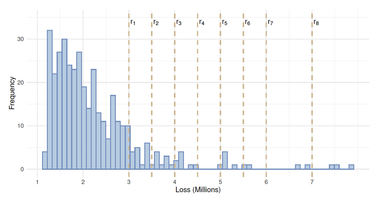
In this section, we illustrate the MA approach to the Secura Re dataset, which consists of left-truncated automobile claims. This dataset is accessible through the R package ltmix, developed by Blostein and Miljkovic (2021). Secura Re losses include 371 claims recorded by the Belgian reinsurance company for the period 1988 to 2001 in 2002 euros. Claims below 1.2 million euros have not been reported to the reinsurer (see Figure 1). Table 1 presents basic summary statistics for Secura Re. The first five basic statistics in this table are reported in millions. The statistics reveal that the mean (2.609) exceeds the median (2.231), and the skewness coefficient of 2.422 indicates a moderate-to-strong positive skewness in the data.

Figure 1.Histogram of Secura Re reinsurance losses with the dashed vertical lines representing eight selected retention levels $\pmb{r \in\{3.0,3.5,4.0,4.5,5.0,5.5,6.0,7.0\}}$.

The Secura Re dataset was used in several actuarial applications related to the estimation of the excess of loss premium, risk measures, and confidence intervals for risk measures; see Verbelen et al. (2015), Reynkens et al. (2017), Blostein and Miljkovic (2019), and Grün and Miljkovic (2023), among others. We employ Secura Re to illustrate the proposed MA approach in the calculation of excess of loss reinsurance premiums at various retention levels. Our interest lies in globally fitting a wide range of possible claim outcomes for Secura Re, as opposed to focusing solely on fitting the tail of the distribution (Beirlant, Matthys, and Dierckx 2001). The objective of this paper is to leverage a comprehensive set of fitting models within a defined model space to address model selection uncertainty.

For the analysis of Secura Re data, a model space is defined consisting of six finite mixture models with a fixed number of components. These models include a single-component lognormal (L), a single-component gamma (G), a two-component lognormal (LL), a two-component gamma (GG), a three-component lognormal (LLL), and a three-component gamma (GGG). For each model considered within this model space, the excess of loss premium is calculated at eight retentions $r$ $\in$ {3.0, 3.5, 4.0, 4.5, 5.0, 5.5, 6.0, 7.0}, expressed in millions of euros. These retention levels are chosen based on their consistency with the literature on modeling the same dataset (see Verbelen et al. 2015) and to ensure a uniform distribution across the range of given losses. Figure 1 shows the histogram of Secura Re losses, with dashed vertical lines indicating the location of the eight retention levels relative to the data. The MA-AIC and MA-BIC are computed, and the summary of the results is presented in Table 2.

It is important to note that the selection of models and the calculation of AIC or BIC weights are based on the likelihood and penalty of complexity, which are independent of the specific retention levels used for premium calculation. Fitting distributions to the data before selecting retention levels ensures that the models used for premium calculations are well suited to the data. This is particularly relevant for Secura Re data, where the same models have been previously explored in the literature (see Blostein and Miljkovic 2019). Understanding the fitted distributions aids in choosing retention levels that are realistic and manageable from a risk management perspective, rather than relying on arbitrary or less-informed choices.

The choice of lognormal and gamma mixture models in our analysis is guided by their superior fit to the Secura Re dataset, demonstrated in prior research by Blostein and Miljkovic (2019) and Verbelen et al. (2015). While other distribution families may be considered, the empirical evidence from previous studies and our preliminary exploratory analysis confirmed that mixtures of lognormals and gammas are sufficient to illustrate our proposed methodology on Secura Re data. In general, these mixtures effectively capture the heavy-tailed nature and multimodality observed in the insurance datasets, making them well suited for excess of loss premium calculations.

The lower portion of Table 2 shows the relative errors in the estimated premium when compared to the empirical results. Four different methods are employed for premium estimation: (i) selecting the best model using the AIC approach (BEST-AIC), (ii) selecting the best model using the BIC approach (BEST-BIC), (iii) using the MA-BIC approach, and (iv) using the MA-AIC approach.

The relative error of each estimation approach compared to its corresponding empirical value is reported, and the results are discussed as follows. The empirical results serve as the benchmark, consistent with previous literature (see Verbelen et al. 2015; Reynkens et al. 2017). However, an alternative benchmark could be selected, such as the best model based on the specified model selection criterion. The AIC and BIC approaches lead to the selection of two different best models. While the BIC approach favors a single lognormal (L), the AIC approach prefers a GG mixture. These results align with previous literature findings, where Blostein and Miljkovic (2019) reported that the lognormal distribution is the best fit for Secura Re based on the BIC criterion, while Verbelen et al. (2015) reported that a two-component Erlang mixture provided the best fit for the same dataset when the AIC criterion was employed in the model selection. It is worth noting that the two-component Erlang mixture can be viewed as a special case of a GG mixture with both components having different shape parameters while sharing a common scale parameter.

The BIC criterion exhibits a preference for a simpler model with fewer parameters, imposing a larger penalty on models with more parameters. As a result, the top model based on BIC weights is the single L model, carrying approximately 96% weight, and the second best is a single-component gamma (G), with about 4% weight. In contrast, the AIC criterion tends to distribute model weights across multiple models. The four models with significant AIC weights are the GG model (47%), the L model (34%), the LL model (13%), and the G model (2%).

Based on the relative error results, the MA-BIC approach demonstrates a slight underestimation of premiums relative to the nonparametric results for all retention levels. Conversely, the MA-AIC approach slightly overestimates the premiums relative to the nonparametric results for the same retention levels. Larger relative errors in premium results are observed as the retention level increases. This is expected because the fit of the tail varies across different models, with some models better suited for the main body of the data and others for the tail. All methods exhibit considerable variability at $r=$ 7.0M, the retention level close to the end of the data range (i.e., maximum observation is 7.899 million).

On average, the MA-AIC premium results closely approximate the nonparametric results across all retention levels except at $r=$ 3.0M. The MA-BIC premium results are closer to the nonparametric results for the retention levels $r=$ 3.0M, $r=$ 3.5M, and $r=$ 7.0M compared to those generated by the MA-AIC approach. However, the MA-AIC premium results are closer to nonparametric results for the retention levels $r=$ 4.0M, $r=$ 4.5M, $r=$ 5.0M, $r=$ 5.5M, and $r=$ 6.0M compared to those generated by the MA-BIC approach.

For the sake of further investigation, we will assume that the best model selected by the BIC approach (L) is excluded from the model space. Thus, the model space under consideration includes only five models: G, GG, GGG, LL, and LLL. The question of interest is: which of the model average estimates will yield results that are closer to the empirical results? Table 3 provides a summary of the results for the five models fitted to Secura Re, along with the model average estimates based on BIC and AIC weights. Table 3 displays the relative errors for the estimated premium when compared to the nonparametric results. Once again, four different methods are employed for premium estimation: (i) BEST-BIC, (ii) BEST-AIC, (iii) MA-BIC, and (iv) MA-AIC approaches. The following discussion delves into the results.

When excluding the L model from the model space of the six models, the G model is selected as the best model by the BIC criterion, while the AIC criterion designates the GG model as the best model. Again, we arrive at two distinct types of models under consideration. Interestingly, the result of the model selection based on the AIC criterion remains the same as when the six original models were used in the model space. The results of the relative errors indicate that the difference between the MA-AIC approach and the nonparametric approach is somewhat the smallest for most retention levels except the first two. Once again, it is observed that the estimates for the highest retention level of 7.0 million have a large relative error and may not be reliable, irrespective of the method employed.

The relative errors based on both the MA-BIC and BEST-BIC methods indicate an underestimation of the premium relative to the empirical results across all retention levels. Conversely, the MA-AIC and BEST-AIC methods tend to overestimate the premium relative to the empirical results.

In summary, it is crucial to emphasize that the MA approach for Secura Re data is demonstrated within a specific class of models, namely a limited space of finite mixture models. This class includes the best-fitting model identified in previous research. If a different class of models, such as composite models, is to be explored, the same MA approach can be easily applied. In fact, several attempts have been made to fit Secura Re data using composite model classes or splicing models (e.g., Reynkens et al. 2017; Grün and Miljkovic 2019). Further, the model space of mixture models can be enlarged to include length- or size-biased mixtures to fit left-truncated data, such as those proposed by Bae and Ko (2020) and Bae and Miljkovic (2024). However, none of the previous research related to alternative model classes has incorporated model uncertainty risk in its applications.

4. Simulation

In this section, a Monte Carlo (MC) simulation study is performed to comprehensively evaluate the performance of the proposed MA approach and to quantify model uncertainty under varying settings and data generating mechanisms similar to those observed in Secura Re. The data generating process is based on the two-component Erlang mixture: a specific form of the GG mixture with shape parameters $\alpha=(5,16)$, a common scale parameter $\theta =360096$, and mixing weights $\omega = (0.97, 0.03)$, reported by Verbelen et al. (2015) to be the best-fitting model. Through this simulation study, the excess of loss premium is computed under four estimation methods for various settings that consider two sample sizes, two truncation points, seven retention levels, and the two simulation scenarios. These simulation settings are summarized as follows.

• Estimation methods: The four estimation methods considered are BEST-AIC, BEST-BIC, MA-AIC, and MA-BIC. The former two methods employ AIC and BIC as model selection criteria, while the latter two methods are grounded in the proposed MA.

• Sample size: The sample size is denoted by $n$ and takes values in the set $n=\{500, 1,000\}$.

• Retention levels: The retention level spans values in the set $R=\{3.0, 3.5, 4.0, 4.5, 5.0, 6.0, 7.0\}$, expressed in millions.

• Simulation scenarios: Two model spaces are considered: $\mathcal{M}_1$ includes six models $\mathcal{M}_1$ $=$ $\{G, GG, GGG, L, LL, LLL\}$, and $\mathcal{M}_2$ encompasses five models $\mathcal{M}_2=\{G, GGG, L, LL, LLL\}$, excluding the GG model. Note that the mixture models with a fixed number of components are considered, similar to those used in modeling Secura Re data.

• Truncation points: The truncation point, denoted by $c$, takes values in the set $c=\{0.8, 1.2\}$, expressed in millions.

• Repetitions: The number of MC runs is set to 1,000, ensuring robust statistical assessment.

To evaluate the four estimation methods, the relative error (RE) is used as the performance measure. For the $i$th level of sample size, the $r$th retention level, the $t$th truncation point, the $k$th method of estimation, and the $l$th repetition in the MC runs, the $RE_{irtkl}$ is calculated using the formula

$$RE_{irtkl} = \frac{{\hat{\pi}_{irtkl}- \pi_{rt}}}{\pi_{rt}},\tag{4.1}$$

where $\hat{\pi}_{irtkl}$ denotes simulated premium value, while $\pi_{rt}$ is the premium based on the true-data generating process. For each combination of simulation settings, a distribution of the RE of the premium is generated relative to the true excess of loss premium based on 1,000 simulation runs. The true excess of loss premium is computed based on the assumed data generating process.

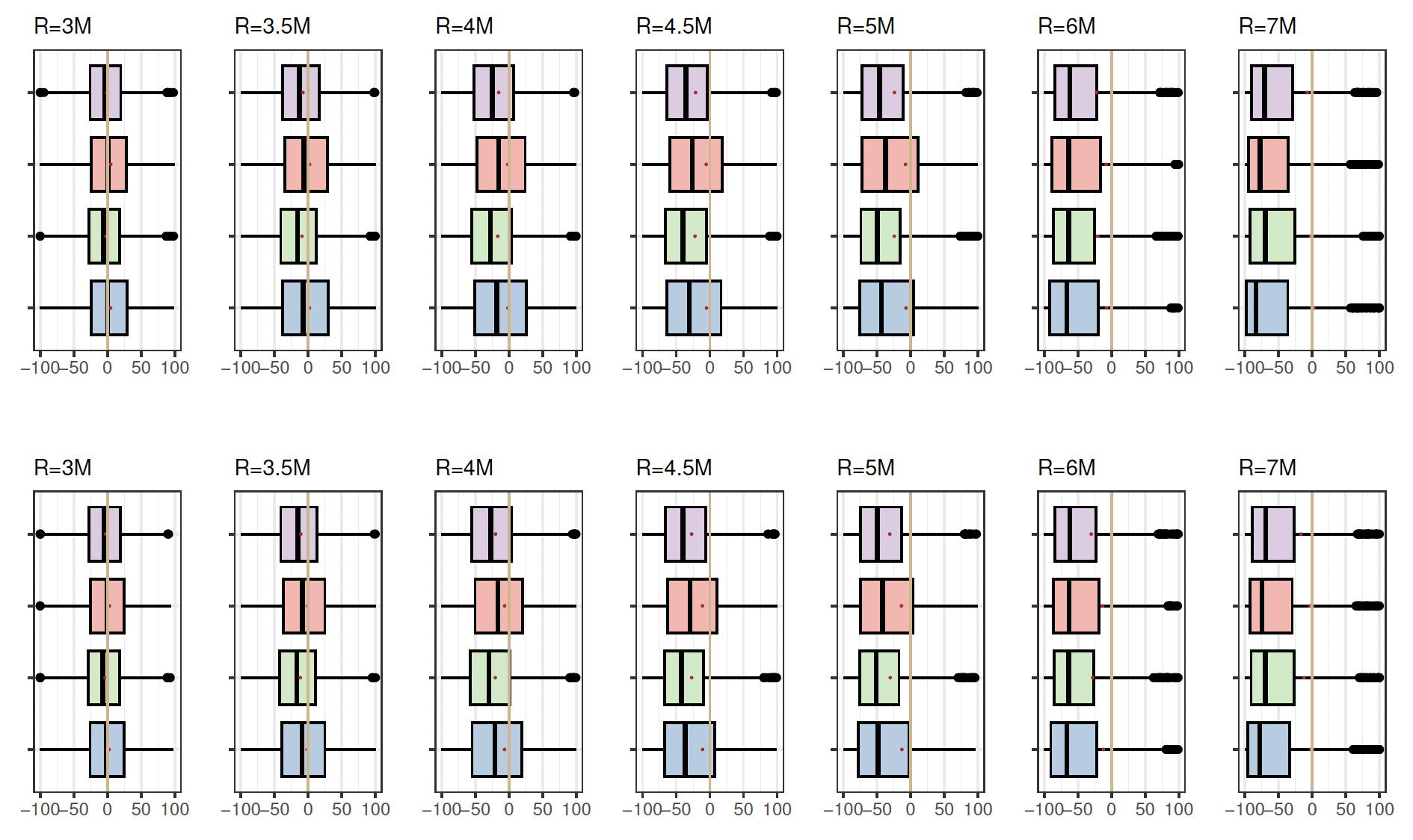
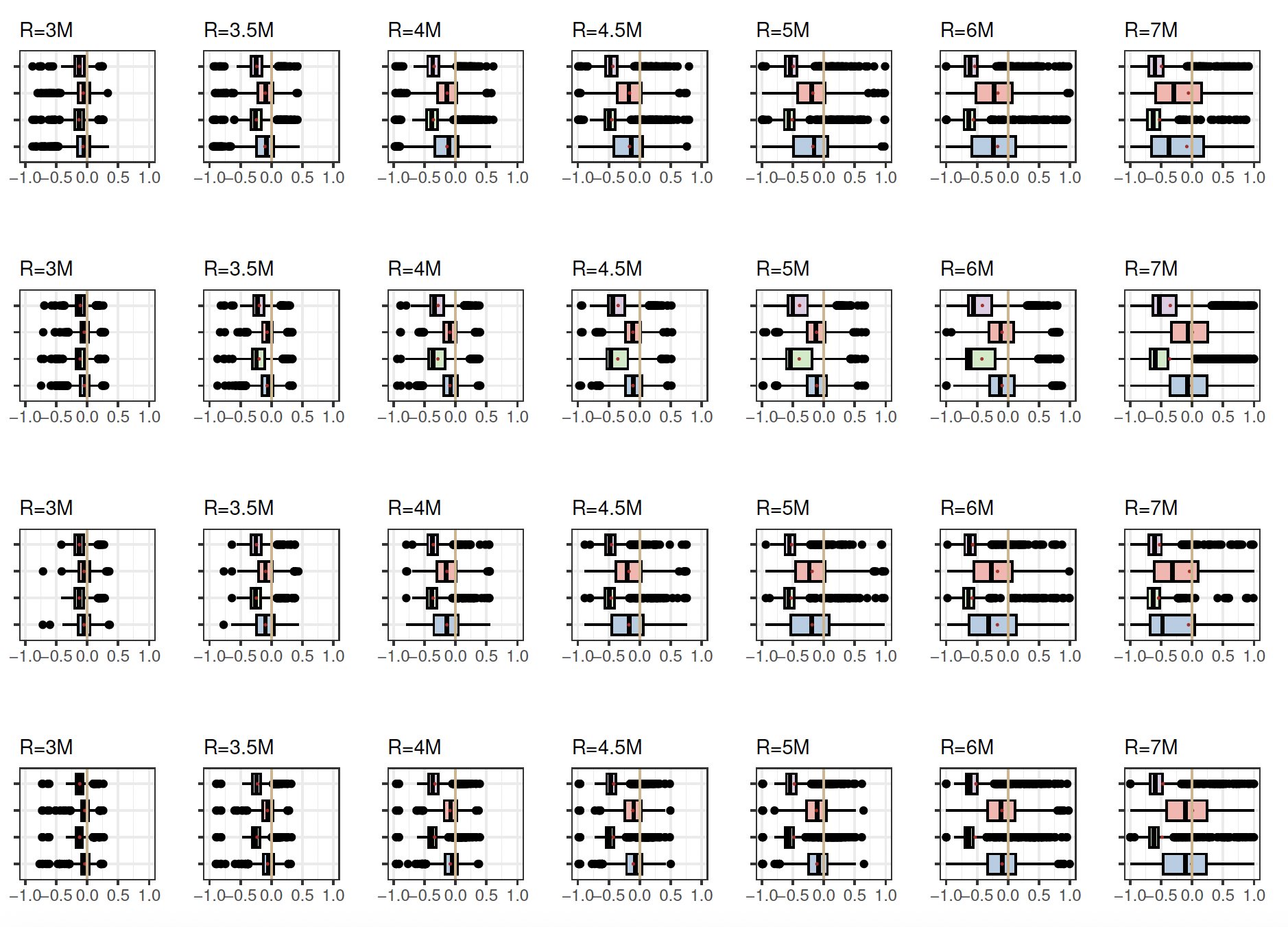
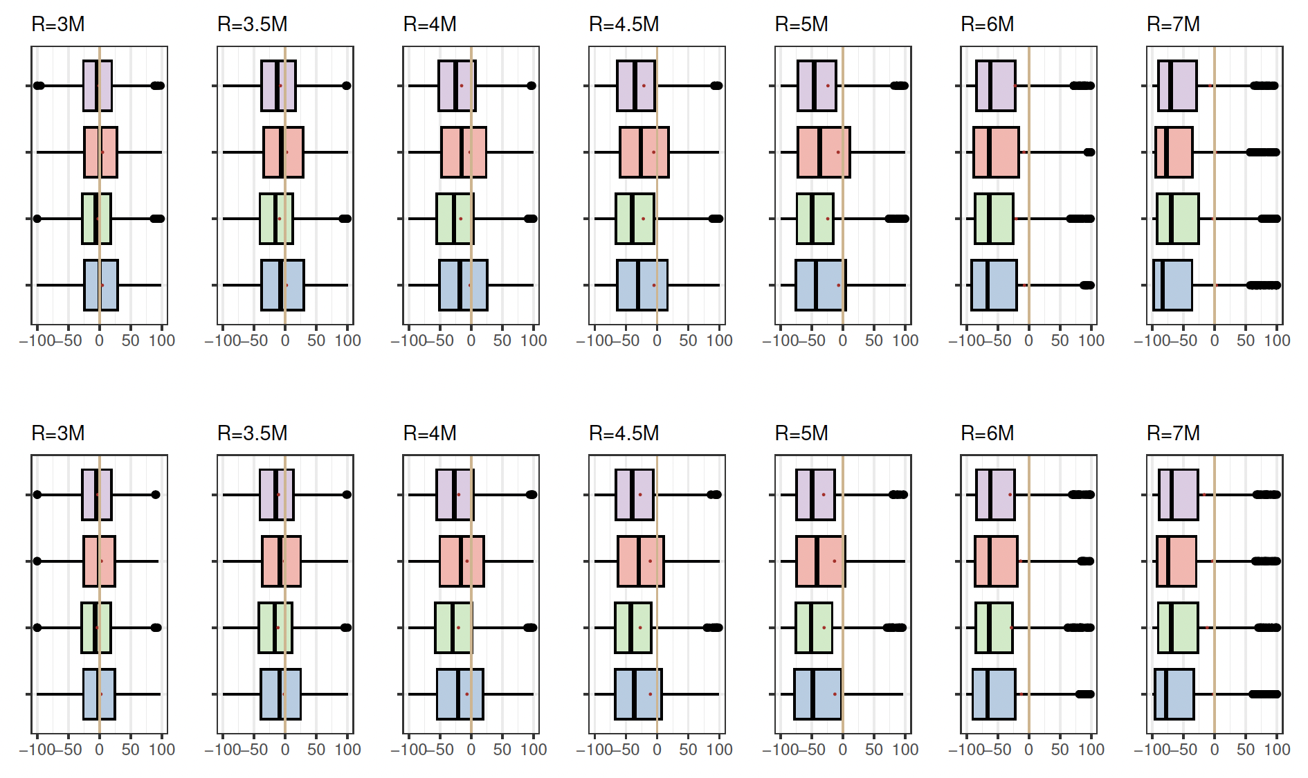
Figure 2 presents box plots illustrating the distributions of RE under various simulation settings, maintaining a fixed truncation point at 1.2. The organization of box plots into four rows corresponds to different combinations of sample size and model space. The first row represents a sample size of $n=500$ with model space $\mathcal{M}_1$, the second row denotes $n=1,000$ with $\mathcal{M}_1$, the third row pertains to $n=500$ with $\mathcal{M}_2$, and the fourth row aligns with $n=1,000$ with $\mathcal{M}_2$. Each row includes box plots for four methods: MA-BIC (soft lavender), MA-AIC (light coral), BEST-BIC (pale green), and BEST-AIC (pale blue). The pale vertical zero-line serves as the reference point, where—ideally, when the estimated premium matches the true premium—RE is equal to zero. Two distinct groups of box plots emerge based on the method: MA-AIC and BEST-AIC exhibit similarities, while MA-BIC and BEST-BIC also share similarities, although these two groups differ in their locations. In many instances, the vertical zero-line is close to one side of the box plot representing MA-AIC and BEST-AIC methods, while it does not intersect MA-BIC and BEST-BIC box plots. Variability is evident with an increase in retention levels and the emergence of outliers. Similarly, a panel plot of box plots in Figure 3 is constructed for the distribution of RE under different simulation settings, with the truncation point fixed at 0.8. Here it is observed that the vertical zero-line intersects both MA-AIC and BEST-AIC box plots for all retention levels, in contrast to MA-BIC and BEST-BIC box plots, which are notably shifted from the vertical reference line.

Figure 2.Panel plot illustrates the summary of relative errors for $\pmb{c=1.2}$. The plot is organized in four rows, each representing a combination of sample size and model space. The first row corresponds to a sample size of $\pmb{n=500}$ with $\pmb{\mathcal{M}_1}$, the second row to $\pmb{n=1,000}$ with $\pmb{\mathcal{M}_1}$, the third row to $\pmb{n=500}$ with $\pmb{\mathcal{M}_2}$, and the fourth row to $\pmb{n=1,000}$ with $\pmb{\mathcal{M}_2}$. Each row contains box plots for four methods: MA-BIC (soft lavender), MA-AIC (light coral), BEST-BIC (pale green), and BEST-AIC (pale blue).

Figure 3.Panel plot illustrates the summary of relative errors for $\pmb{c=0.8}$. The plot is organized in four rows, each representing a combination of sample size and model space. The first row corresponds to a sample size of $\pmb{n=500}$ with $\pmb{\mathcal{M}_1}$, the second row to $\pmb{n=1,000}$ with $\pmb{\mathcal{M}_1}$, the third row to $\pmb{n=500}$ with $\pmb{\mathcal{M}_2}$, and the fourth row to $\pmb{n=1,000}$ with $\pmb{\mathcal{M}_2}$. Each row contains box plots for four methods: MA-BIC (soft lavender), MA-AIC (light coral), BEST-BIC (pale green), and BEST-AIC (pale blue).

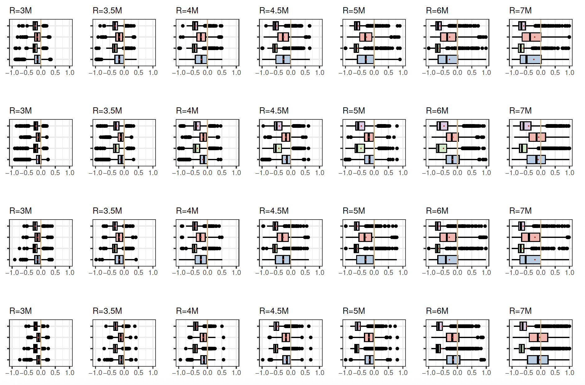
The magnitude of RE shows a decrease when the truncation point is lowered from 1.2 to 0.8, corresponding to a reduction in the left tail area of the distribution. Notably, when the true model is encompassed within the model space and the sample size is small ($n=500$), the MA-AIC method yields slightly superior results compared to the BEST-AIC approach. However, with a larger sample size ($n=1,000$), MA-AIC outperforms BEST-AIC at certain retention levels, particularly in the right tail. It is observed that the variability in the distribution of REs increases with a higher retention level. Notably, smaller variability is noted for retention level 3.0M, while the largest variability is reported for 7.0M (tail area).

The tabulated values for the average RE, denoted as $\overline{RE}$, are summarized in Table 6 in Appendix C. The standard deviations of the RE for each distribution across the combination of settings are presented in Table 7 (Appendix C). The standard deviation increases with an increase in retention level across all other simulation settings and serves as an indicator of the uncertainty associated with the premium estimates. Specifically, the standard deviation of the RE distribution can be used to quantify the uncertainty in premium estimation at each retention level. It is also important to note that the MA-AIC and MA-BIC methods exhibit lower variability, on average, across all simulation settings, compared to their counterparts (BEST-AIC and BEST-BIC).

Table 4 illustrates the frequency of the correct model being selected over 1,000 MC runs when the true model is included in the model space. The AIC appears to select the correct model (GG) most of the time, whereas the BIC tends to favor the simpler model (L) regardless of the truncation point and the sample size.

When the true model is excluded from the model space, the frequency of the best model selected is summarized in Table 5 for both AIC and BIC model selection criteria. The BIC consistently selects a single-component lognormal as the best model regardless of the truncation point and the sample size. The AIC tends to select several candidate models, among which a single lognormal is frequently chosen, particularly when the truncation point is 0.8 and 1.2 with a sample size of 500. A single-component gamma is never selected by either AIC or BIC. The AIC tends to select the GGG model more frequently than the BIC approach, even though the true model GG, which is excluded from $\mathcal{M}_2$, consists of the same component distributions.

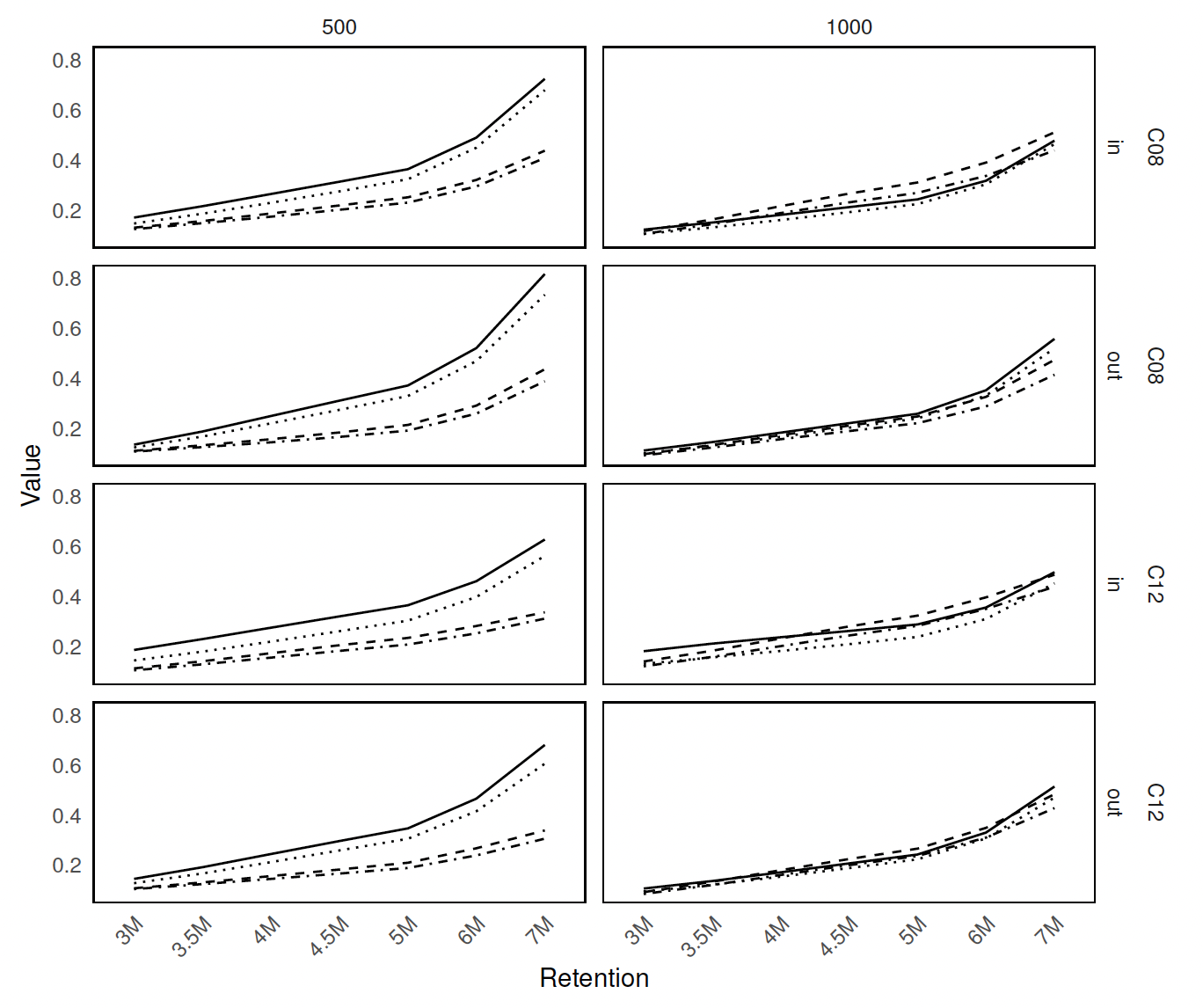
Figure 4 shows the panel plot consisting of multiple line plots of $\overline{RE}$ under various simulation settings. The organization of line plots into four rows corresponds to different combinations of sample size, model space, and truncation point. The first column represents a sample size of $n=500$, while the second column represents sample size $n=1,000$. The first two rows correspond to truncation point 0.8, while the last two rows show the results for truncation point 1.2. Sample space is labeled as “in” for $\mathcal{M}_1$ and “out” for $\mathcal{M}_2$. There are four line styles denoting one of the four estimation methods: BEST-AIC (solid), BEST-BIC (dashed), MA-AIC (dotted), and MA-BIC (dot-dashed). This panel plot reveals a common trend among all estimation methods: none of them yields an $\overline{RE}$ greater than zero. The results validate the analysis of real data where the best-selected models seem to slightly underestimate the empirical results. MA-AIC and BEST-AIC show significantly smaller $\overline{RE}$s across all retention levels compared to the BEST-BIC and MA-BIC methods. Additionally, from Figure 4 we observe that an increase in sample size seems to decrease $\overline{RE}$. Lowering the left-truncation point has an impact of reducing the $\overline{RE}$. This is expected, since lowering the truncation point would allow the inclusion of more observations that were previously excluded due to being below the original truncation threshold. This inclusion of additional data points can provide more information about the lower tail of the distribution as well as the overall distribution of the data, leading to improved accuracy of the premium estimates based on this distribution.

Figure 4.Line plots of $\overline{R E}$ organized for all combinations of the simulation settings as follows: sample size (in columns): 500, 1,000; method of estimation: BEST-AIC (solid), MA-AIC (dotted), BEST-BIC (dashed), and MA-BIC (dotdashed); truncation point denoted as C08 and C12 for 0.8 and 1.2, respectively (across two rows); two scenarios labeled as “in” corresponding to $\mathcal{M}_1$ and “out” corresponding to $\mathcal{M}_2$ (by row).

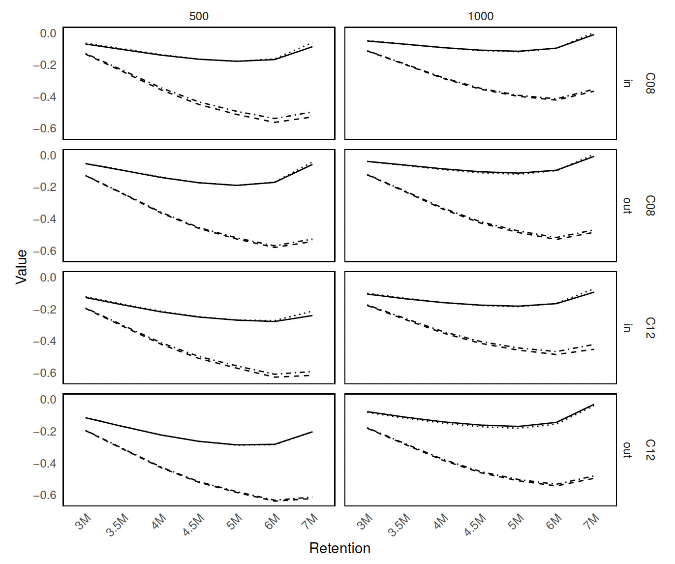
Figure 5 displays the standard deviation of RE values across retention levels, organized similarly to Figure 4. Overall, the standard deviation of RE tends to increase with higher retention levels—especially noticeable with smaller sample sizes ($n=500$). For these, the variability in RE is notably lower for BEST-BIC (dashed line) and MA-BIC (dot-dashed line) than for BEST-AIC (solid line) and MA-AIC (dotted line). MA-BIC shows slightly lower variability than BEST-BIC. For larger sample sizes ($n=1,000$), there is less variability in RE across methods. Considering $\mathcal{M}_1$, MA-AIC shows the lowest standard deviation across most retention levels, while for $\mathcal{M}_2$, MA-BIC demonstrates the smallest variability in RE.

Figure 5.Line plots show the standard deviation of RE values organised for all combinations of the simulation settings as follows: sample size (in columns): 500, 1,000; method of estimation: BESTAIC (solid), MA-AIC (dotted), BEST-BIC (dashed), and MA-BIC (dotdashed); truncation point denoted as C08 and C12 for 0.8 and 1.2, respectively (across two rows); two scenarios labeled as “in” corresponding to $\mathcal{M}_1$ and “out” corresponding to $\mathcal{M}_2$ (by row).

To assess the performance of the proposed approach with a small sample size, additional simulation runs ($N=1,000$) were conducted with $n=50$ and a truncation point of $c=1.2$. The data generating process remained consistent with the original setup, based on a two-component GG mixture with shape parameters $\alpha=(5,16)$, a common scale parameter $\theta =360096$, and mixing weights $\omega = (0.97, 0.03)$. Two scenarios were considered: “in” corresponding to $\mathcal{M}_1$ and “out” corresponding to $\mathcal{M}_2$. The results are summarized in Appendix C. Table 8 presents the mean of the RE distribution across different settings, while Table 9 reports the standard deviation. Compared to the results obtained with moderate and large sample sizes, we observe substantial variability across all retention levels, regardless of the premium estimation approach. Figure 6 displays box plots organized into two rows corresponding to the two model spaces. The variability increases with higher retention levels, accompanied by a growing number of outliers. For retention levels in the tail of the distribution, the variability becomes so large that the results may be considered unreliable. Moreover, small sample sizes introduce additional uncertainty in parameter estimation, a well-known phenomenon in statistical inference, further compounding the challenges of working with limited data.

It is important to note that a simulation study can be used to quantify model uncertainty by analyzing the standard deviation of the RE distribution associated with the premium estimates. However, directly quantifying model uncertainty with real data is more challenging, as the true values are not available for comparison. In such cases, one potential approach is to simulate data under conditions similar to those in the real data and apply the same methods used in the simulation study, as demonstrated in this section of the paper. This approach allows for assessing how the model behaves under various scenarios and better quantifying the uncertainty associated with the MA process in a real-world context.

5. Conclusion and discussion

The field of loss modeling is extensive, encompassing a wide array of model classes for modeling insurance losses. However, there has been relatively little research on MA to address the uncertainty inherent in selecting the best-fitted models, which can significantly impact critical risk management decisions.

This paper introduces an approach for addressing uncertainty in model selection and improving the accuracy of estimated excess of loss premiums. The proposed method involves MA for estimating the excess of loss premium when finite mixture models, utilizing gamma and lognormal component distributions, are considered. Furthermore, we have derived closed-form formulas for computing the model average premium using AIC and BIC weights, which are based on the gamma and lognormal mixtures, fitted to left-truncated insurance losses.

When estimating the excess of loss premium using Secura Re data, we found that the model average estimators based on either AIC or BIC weights perform slightly better than individual models selected solely based on AIC or BIC criteria. Most importantly, model average estimators account for model uncertainty, an important factor when multiple models are involved in analyzing loss data.

Through extensive simulations, we discovered that the MA-BIC method exhibits the least variability across all retention levels when the sample size is small. On average, both MA-AIC and AIC tend to approximate the true model more closely across all simulation settings, with MA-AIC showing slight improvements in the results. Our simulation study validates findings observed in modeling real datasets, as the shape of the simulated data closely resembles that of Secura Re data.

The reader is advised that while this study focuses on lognormal and gamma mixture models due to their strong empirical fit to the Secura Re dataset, other distribution families can also be considered based on the specific characteristics of the real data. It is important to assess the distributional fit of the data before selecting the model, as different datasets may exhibit different behaviors that could be better captured by alternative distributions. As such, we encourage practitioners to explore a wide range of distribution families when analyzing their own datasets, adjusting their model selection based on the specific features of the data at hand. Based on the considered distribution families, the excess of loss premium can be computed using the proposed MA approach to account for model uncertainty and improve the reliability of the premium estimates, offering a more robust solution compared to relying on a single model.

Other methods for averaging models can be explored; for instance, for small $n$ a corrected version of AIC ($AIC_C$) exists that provides stronger penalty for small sample sizes and stronger than BIC for very small sample sizes. $AIC_C$ is reported by Burnham and Anderson (2004) to have better small-sample behavior. Further developments are being made, and new forms of information criteria have been proposed. The Watanabe-Akaike (or widely applicable) information criterion (WAIC; see Watanabe and Opper 2010) is an attempt from Bayesian statistics to emulate a cross-validation analysis. While WAIC is preferred to the deviance information criterion, a direct leave-one-out criterion is now recommended (see Spiegelhalter et al. 2002 and Vehtari, Gelman, and Gabry 2016, among others). These developments highlight the ongoing efforts to refine and improve MA techniques.

There is significant potential to extend the methodology proposed in this paper to encompass premium calculations for other types of reinsurance contracts. For example, in surplus share reinsurance, which covers a percentage of each loss up to a certain limit, one can utilize the MA approach. By averaging the loss ratios from various models using AIC or BIC weights, the reinsurance premium can be determined while accounting for model uncertainty. Another potential application is in parametric (or index-based) insurance, which pays out based on predefined trigger events, such as rainfall levels or earthquake magnitudes. The premium can be estimated using model-averaged predictions of the trigger event’s probability. In this context, AIC or BIC weights allow for averaging the predictions of the event’s occurrence to determine the premium. Additionally, catastrophe bonds (cat bonds) are used by insurers to transfer risk to the capital markets. The premium for these bonds can be influenced by models estimating the frequency and severity of catastrophic events. The expected loss rate used in premium calculations can be derived from model-averaged estimates of catastrophe risk, with AIC or BIC weights applied to average predictions of catastrophe loss from various models. The methodology in this paper can also be extended to a layer reinsurance contract, where the reinsurer covers losses within a specific range, between a lower retention point and an upper retention point. The premium for such a contract can be derived by integrating over the range of losses that the reinsurer is liable for.

One avenue for future work would be to explore the use of the FIC approach in calculation of the excess of loss premium. Future research could explore modifications to FIC to enhance its applicability to premium estimation, including the potential development of a smoothed or regularized approach that could impose constraints to ensure consistency across different retention levels. Further investigation into the asymptotic properties of FIC in the context of excess loss pricing, particularly under different loss distribution assumptions, could also provide valuable insights. Exploring these directions would help refine the use of FIC in actuarial applications.

Finally, the proposed framework is based on the expected premium principle, but it can be carefully extended to other premium principles, such as the variance premium principle (which adds a variance term to adjust the premium for risk variability) and the standard deviation premium principle (which considers the standard deviation of the loss distribution). Challenges may arise when combining the mean and variance (or standard deviation), particularly in terms of computational complexity. Additionally, careful consideration should be given to the model weights, as ideally they would reflect not only the goodness of fit for the expected loss but also the variability captured by the model (i.e., the variance and standard deviation).

Acknowledgment

The author sincerely appreciates the thoughtful comments and suggestions from the editor and two anonymous reviewers, which have helped enhance the quality of this manuscript. The author is also grateful to Dr. Nikita Barabanov and Dr. Seonjin Kim for their insightful feedback on an earlier version of this work.