A Comparison: Some Approximations for the Aggregate Claims Distribution

1. Introduction

Aggregate claim distributions have been widely discussed in the actuarial literature. For example, see Heckman and Meyers (1983), Teugels (1985), Pentikäinen (1987), Papush, Patrik, and Podgaits (2001), Hardy (2004), and Reijnen, Albers, and Kallenberg (2005). In the context of insurance theory, the aggregate claims can be viewed as a sum of individual claim amounts for a random number of claim counts over a fixed time-period. In other words, it can be represented as a sum of individual claim amounts for a random number of claim counts over a fixed time-period. In other words, it can be represented as a sum (S) of individual claim amounts $X_1, X_2, \ldots, X_N$, where $N$ is the random number of claim counts over a fixed time period. Conditional on $N=n$, the random variables $X_1, X_2, \ldots, X_N$ are assumed to be positive, mutually independent, and identically distributed. It is also assumed that the common distribution of $X_i$’s is independent of $N$. One can easily write the cumulative distribution function (c. d.f) of aggregate claims random variable (S) as

$$\begin{aligned} C F_{s}(x) & =P(S \leq x) \\ & =\sum_{n=0}^{\infty} P(N=n) P\left(X_{1}+X_{2}+\ldots+X_{N} \leq x \mid N=n\right) . \end{aligned} \tag{1.1}$$

The computation of this compound distribution function or corresponding tail probability or probability density function is generally quite cumbersome. For most combinations of distributions of N and the X_i’s, the exact distribution of S is not available analytically, but the above distributional values may be obtained numerically. For discrete severity distributions, one often uses the well-known recursive method introduced by Panjer (1981) to evaluate the aggregate claims distribution. For exponential severities, simple analytical results for exact probabilities can easily be obtained (Klugman, Panjer, and Willmot 2012). For other cases, the computation in (1.1) requires tedious numerical integrations. In this situation, one often prefers to use an approximate distribution to avoid the computational complexity of distributional values. Several approximations have been developed and studied by many authors in the actuarial literature. Here, we have considered only four of them, which are NP₂, gamma, IG, and gamma-IG mixture approximations. The NP₂ approximation provided by Pesonen (1969) and the gamma approximation introduced by Bohman and Esscher (1963) are well known to the actuarial community. Chaubey, Garrido, and Trudeau (1998) introduced IG and gamma-IG mixture approximations to aggregate claims distribution. They compared these approximations with NP₂ and gamma approximations for some choices of the distributions of claim counts and claim sizes. The authors stated that the gamma-IG mixture approximation uniformly improves the accuracy, especially in the tails. However, this approximation requires numerical evaluation of incomplete gamma functions. Seri and Choirat (2015) have studied a number of approximations for compound Poisson processes only and discussed their findings. Alhejaili and Abd-Elfattah (2013) discussed the saddlepoint approximation, introduced by Lugannani and Rice (1980), for some stopped-sum distributions and noted that the approximation shows a great accuracy compared to exact distribution. Recently, Thiagarajah (2017) has studied extensively the saddlepoint approximation to the tail probabilities of aggregate claims for various combinations of claim counts and claim severity distributions. The author has compared the approximate tail probabilities with the exact probabilities and concluded that the accuracy of this approximation is quite good in all applications considered in the paper.

The paper is organized as follows: In Section 2 we present a brief description of five of the above approximations to the cumulative distribution function of aggregate claims. In Section 3, we compare the accuracy of these approximations numerically in terms of relative errors for various combinations of claim count and claim size distributions. The relative error is computed as (approximate probability − exact probability)/exact probability. If the exact probabilities are not available analytically, we obtain them through simulations. In that case, we first generate a random number N from a claim count distribution, and then generate N random values from a claim size distribution. The aggregate claim amount (S) is taken as the sum of those N values. Each probability is based on 100,000 replications. The final section contains the conclusion.

2. Approximations

In this section, we provide five approximations for the distribution of the aggregate claims. We need mean, variance, skewness, or kurtosis of the aggregate claims distribution for these approximation methods. These quantities can easily be obtained from the cumulant generating function, which is the natural logarithm of the moment generating function. Let us denote the cumulant generating function (c.g.f) of $S$ as $C_S(t)$. Then, we can write the mean $=\mu_s=C_S^{(1)}(0)$, the variance $=\sigma_S^2=\mu_2(s)=C_S^{(2)}(0)$, the third central moment $\mu_3(s)=C_S^{(3)}(0)$, and the fourth central moment $\mu_4(s)=C_S^{(4)}(0)+3\left(C_S^{(2)}(0)\right)^2$. Now, we express the skewness as $\gamma_s=\frac{\mu_3(s)}{\sqrt{\left(\mu_2(s)\right)^3}}$ and the kurtosis as $\kappa_S=\frac{\mu_4(s)}{\left(\mu_2(s)\right)^2}$.

2.1. NP₂ approximation

Using the well-known central limit theorem, one can approximate the aggregate claims distribution by a normal distribution. This method works only for a large volume of risks. Pesonen (1969) provided the following expression, which is called normal power (NP₂) approximation, as an adjustment to the normal approximation:

$$C F(x) \approx \Phi\left[\sqrt{1+\frac{9}{\gamma_{s}^{2}}+\frac{6 Z}{\gamma_{s}}}-\frac{3}{\gamma_{s}}\right], \tag{2.1}$$

where $Z=\frac{\left(x-\mu_{s}\right)}{\sigma_{s}}$ and γ_S is the skewness of S. The μ_S and σ_S are the mean and the standard deviation of S. Pentikäinen (1977) claims that this approximation method gives very satisfactory results, provided that the skewness of the distribution of interest is very small.

2.2. Gamma approximation

Bohman and Esscher (1963) discussed this approximation, which is based on incomplete gamma function. Here, the aggregate claims distribution is approximated by a simple gamma distribution. An improvement to the simple gamma distribution is referred to as the gamma approximation, which is given in (2.2).

$$C F(x) \approx \frac{1}{\Gamma(\alpha)} \int_{0}^{\alpha+Z \sqrt{\alpha}} e^{-y} y^{a-1} d y, \tag{2.2}$$

where $Z=\frac{\left(x-\mu_{s}\right)}{\sigma_{s}}$ and $\alpha=\frac{4}{\gamma_{s}^{2}}$ . Seal (1977) commented that the NP₂ method should be abandoned in favor of this gamma approximation. Gendron and Crépeau (1989) claimed that this approximation provides satisfactory results when the claim size distribution is inverse Gaussian. Pentikäinen (1977) stated that both NP₂ and gamma approximations provide similar outcomes, and both are acceptable approximations when the skewness of the aggregate claims distribution is less than two.

2.3. IG approximation

Chaubey, Garrido, and Trudeau (1998) proposed this approximation, which was developed by matching the moments, as in the previous two methods. They approximated the random variable S by a shifted IG(m, b) distribution by matching the first three central moments. This means

$$C F(x) \approx G_{m, b}\left(x-x_{0}\right), \tag{2.3}$$

where G is the cumulative probability of the shifted IG distribution. The parameters m and b can be written as $m=\frac{3\left[C_{s}^{(2)}(0)\right]^{2}}{C_{s}^{(3)}(0)}$, $b=\frac{C_{s}^{(3)}(0)}{3 C_{s}^{(2)}(0)}$, and x₀ = C_S⁽¹⁾(0) − m. The authors claim that the approximation is almost as good as the gamma approximation.

2.4. Gamma-IG mixture approximation

Chaubey, Garrido, and Trudeau (1998) also introduced this approximation as a weighted average of gamma and IG approximations. The approximation was given as

$$C F(x) \approx w C F_{1}(x)+(1-w) C F_{2}(x), \tag{2.4}$$

where $w=\frac{\kappa_{S}-\kappa_{F_{2}}}{\kappa_{F_{1}}-\kappa_{F_{2}}}$, and κ stands for kurtosis. This is an improvement of the accuracy of both gamma and IG approximations.

2.5. Saddlepoint approximation

Lugannani and Rice (1980) introduced a method based on the saddlepoint technique, which can be applied to continuous and discrete distributions. It is a simple and accurate approximation for distribution function, which avoids any integration. For continuous severity distributions of X_i’s, the saddlepoint approximation to the cumulative distribution function of S can be written as

$$C F(x) \approx\left\{\begin{array}{ll} \Phi(\hat{\omega})+\phi(\hat{\omega})\left\{\frac{1}{\hat{\omega}}-\frac{1}{\hat{u}}\right\}, & x \neq \mu \\ \frac{1}{2}+\frac{C_{S}^{(3)}(0)}{6 \sqrt{2 \pi\left(C_{S}^{(2)}(0)\right)^{3}}}, & x=\mu \end{array}\right. \tag{2.5}$$

where $\Phi$ and $\varphi$ are the respective cumulative distribution function and the probability density function of a standard normal random variable, $\mu$ is the mean of the distribution, $\hat{w}=\operatorname{sgn}(\hat{t}) \sqrt{2\left\{\hat{t} x-C_S(\hat{t})\right\}}$, and $\hat{u}=\hat{t} \sqrt{C_S^{(2)}(\hat{t})}$. The saddlepoint $\hat{t}=\hat{t}(x)$ is the unique solution to the equation $C_S^{(1)}(\hat{t})=x$. For more mathematical details of this approximation, we refer the readers to Lugannani and Rice (1980) and Daniels (1987).

3. Some compound distributions

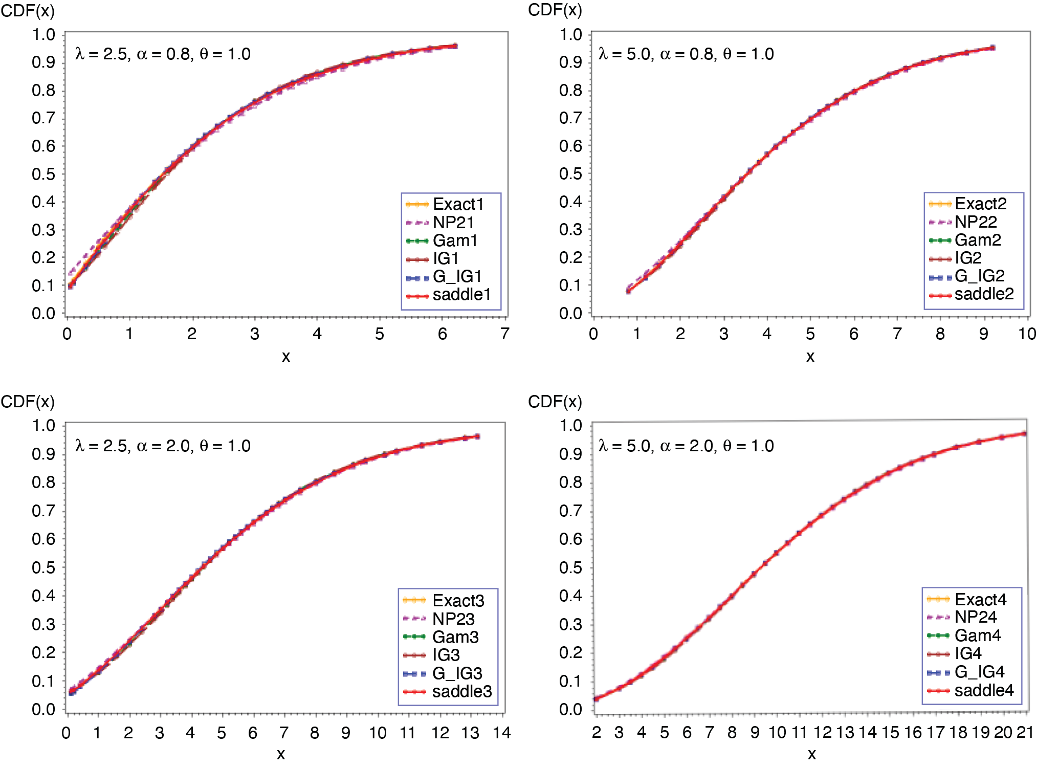
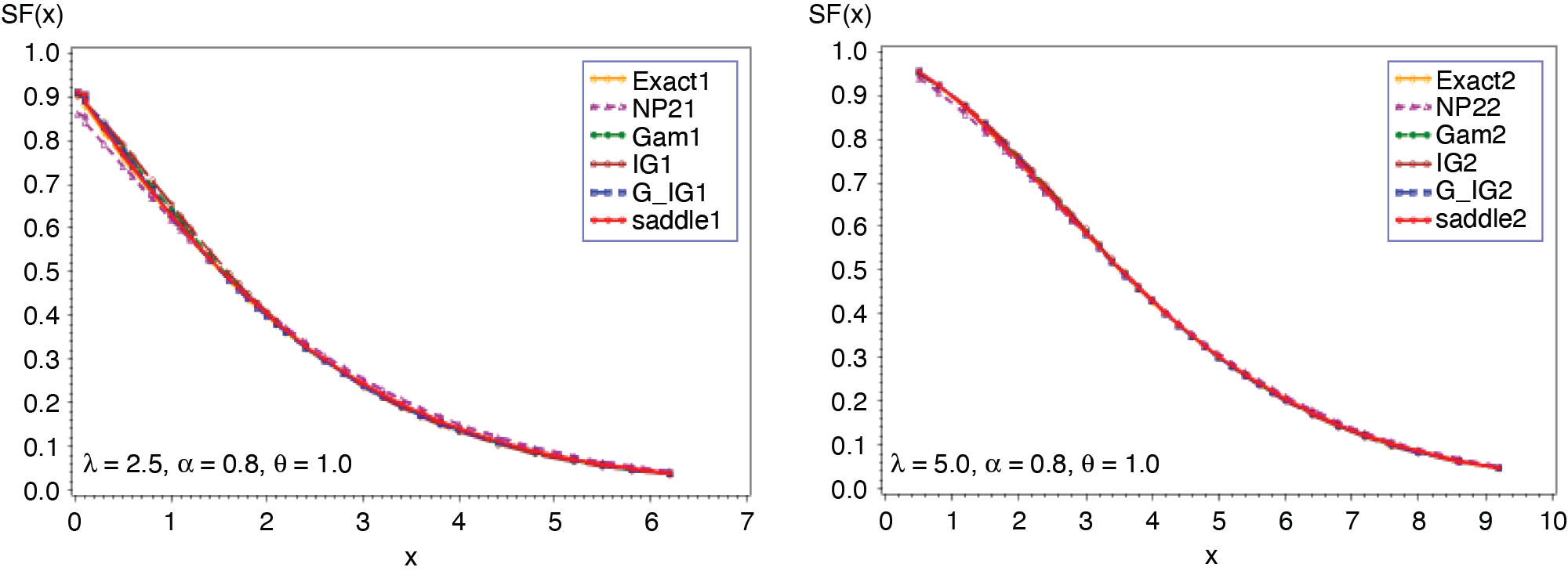
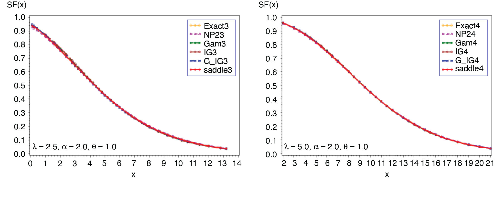
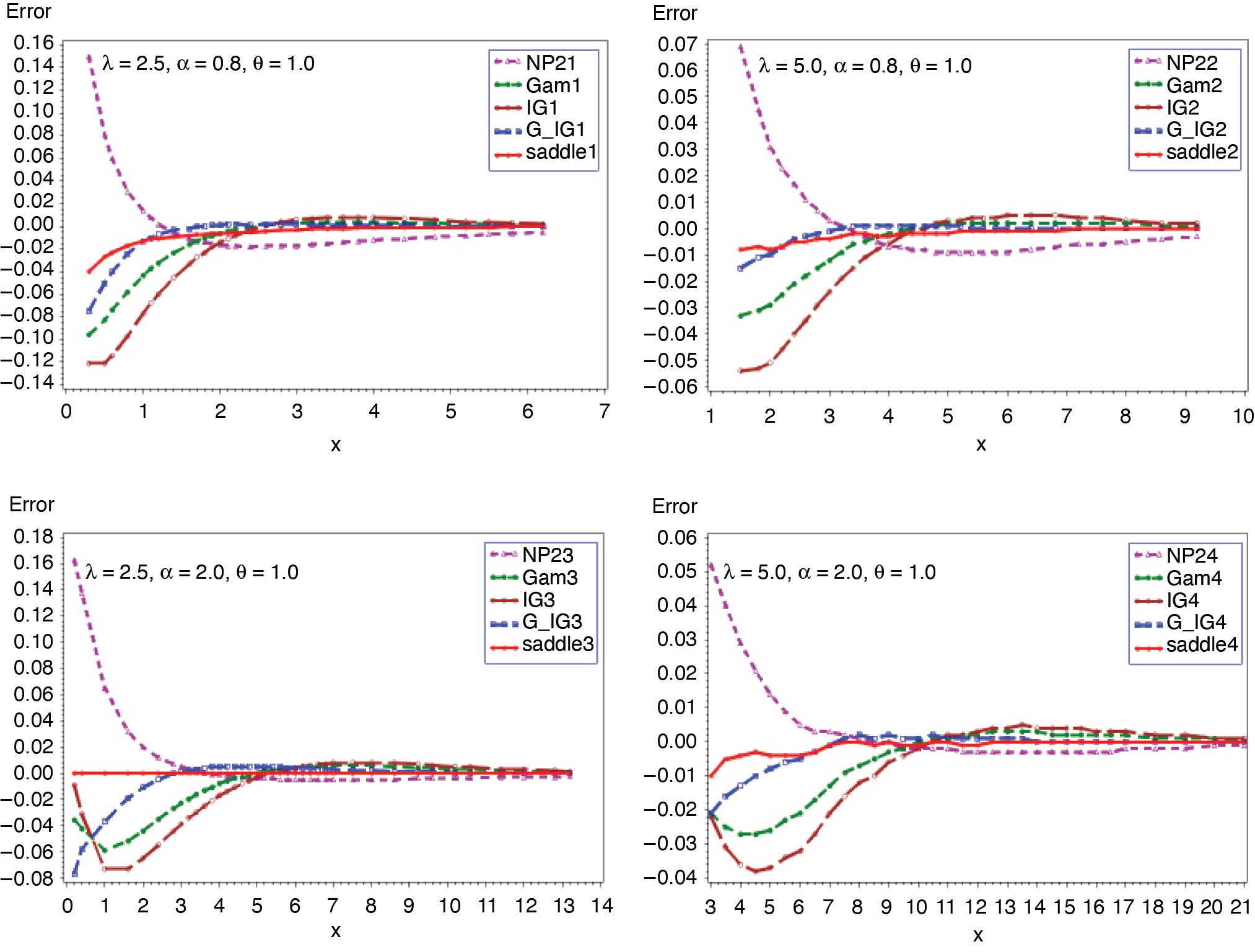
3.1. Poisson-gamma distribution (λ, α, θ)

In this example, the number of claims has a Poisson distribution with parameter λ, and the common severity distribution is gamma with parameters α and θ. The cumulant generating function (c.g.f.) of S and its first derivative are as follows:

$$C_{S}(t)=\lambda\left[(1-\theta t)^{-\alpha}-1\right], \quad t<1 / \theta \tag{3.1}$$

$$C_{S}^{(1)}(t)=\lambda \alpha \theta(1-\theta t)^{-(\alpha+1)} . \tag{3.2}$$

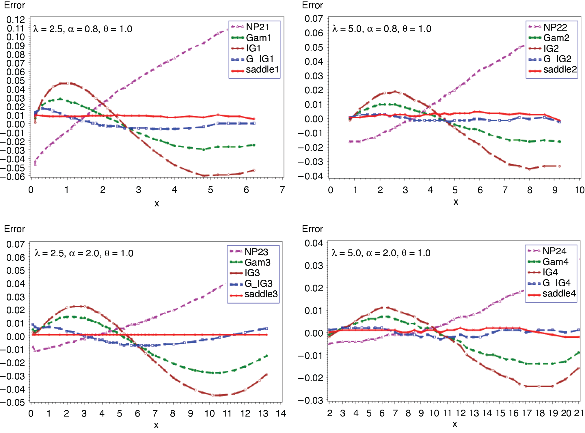
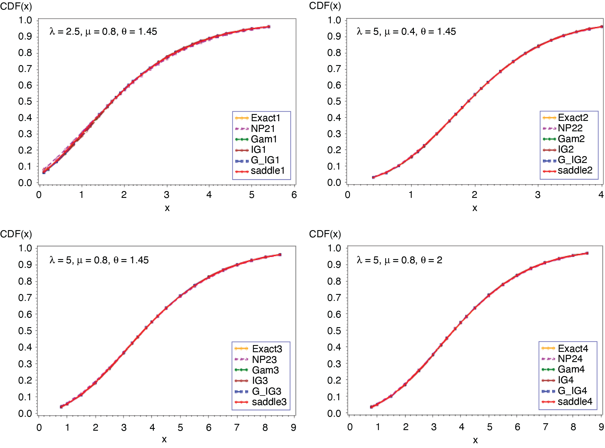
Expression in (3.2) yields the saddlepoint $\hat{t}$ as $\hat{t}=\frac{1}{\theta}\left[1-\left(\frac{\lambda \alpha \theta}{x}\right)^{\frac{1}{\alpha+1}}\right]$. From (3.1), we obtain the first four moments which are given as $\mu \mathrm{s}=\lambda \alpha \theta ; \mu_2(\mathrm{~s})= \lambda \alpha(\alpha+1) \theta^2$ ; $\mu_3(s)=\lambda \alpha(\alpha+1)(\alpha+2) \theta^3$ ; $\mu_4(s)= \lambda \alpha(\alpha+1)[(\alpha+2)(\alpha+3)+3 \lambda \alpha(\alpha+1)] \theta^4$. Figures 1 and 2 display the cumulative (CF) and the tail probabilities (SF) for different parameter combinations. Figures 3 and 4 illustrate the relative errors for those combinations. For all cases, the approximation (2.5) gives excellent results, followed by gamma-IG mixture approximation.

Figure 1.CF: Poisson-gamma $(\lambda, \alpha, \theta)$

Figure 2.SF: Poisson-gamma $(\lambda, \alpha, \theta)$

Figure 2.SF: Poisson-gamma $(\lambda, \alpha, \theta)$ (Continued)

Figure 3.CF relative error: Poisson-gamma $(\lambda, \alpha, \theta)$

Figure 4.SF Relative error: Poisson-gamma $(\lambda, \alpha, \theta)$

3.2. Poisson-IG distribution (λ, μ, θ)

In this example, the claim count random variable (N) follows a Poisson distribution with parameter λ, and the common severity random variable (X) has inverse Gaussian distribution with parameters μ and θ, defined as in Klugman, Panjer, and Willmot (2012). The c.g.f of S and its first derivative are

$$C_{S}(t)=\lambda\left\{\exp \left[\frac{\theta}{\mu}(1-\sqrt{v})\right]-1\right\}, \quad t<\frac{\theta}{2 \mu^{2}} \tag{3.3}$$

$$C_{S}^{(1)}(t)=\frac{\lambda \mu}{\sqrt{v}} \exp \left[\frac{\theta}{\mu}(1-\sqrt{v})\right], \tag{3.4}$$

where $v=1-\frac{2 t \mu^2}{\theta}$. The saddlepoint, $\hat{t}=\hat{t}(x)$, can be obtained by solving the following equation numerically:

$$\frac{\ln v}{2}+\frac{\theta \sqrt{v}}{\mu}=\frac{\theta}{\mu}-\ln \left(\frac{x}{\lambda \mu}\right) . \tag{3.5}$$

Equation (3.3) yields the following quantities:

$$\begin{array}{l} \mu s=\lambda \mu \\ \mu_{2}(s)=\lambda(\mu+\theta) \mu^{2} / \theta \\ \mu_{3}(s)=\lambda\left(3 \mu^{2}+3 \mu \theta+\theta^{2}\right) \mu^{3} / \theta^{2} \\ \mu_{4}(s)=\lambda\left[\begin{array}{c} 15 \mu^{2}(\mu+\theta)+\theta^{2}(6 \mu+\theta) \\ +3 \lambda \theta(\mu+\theta)^{2} \end{array}\right] \mu^{4} / \theta^{3} . \end{array}$$

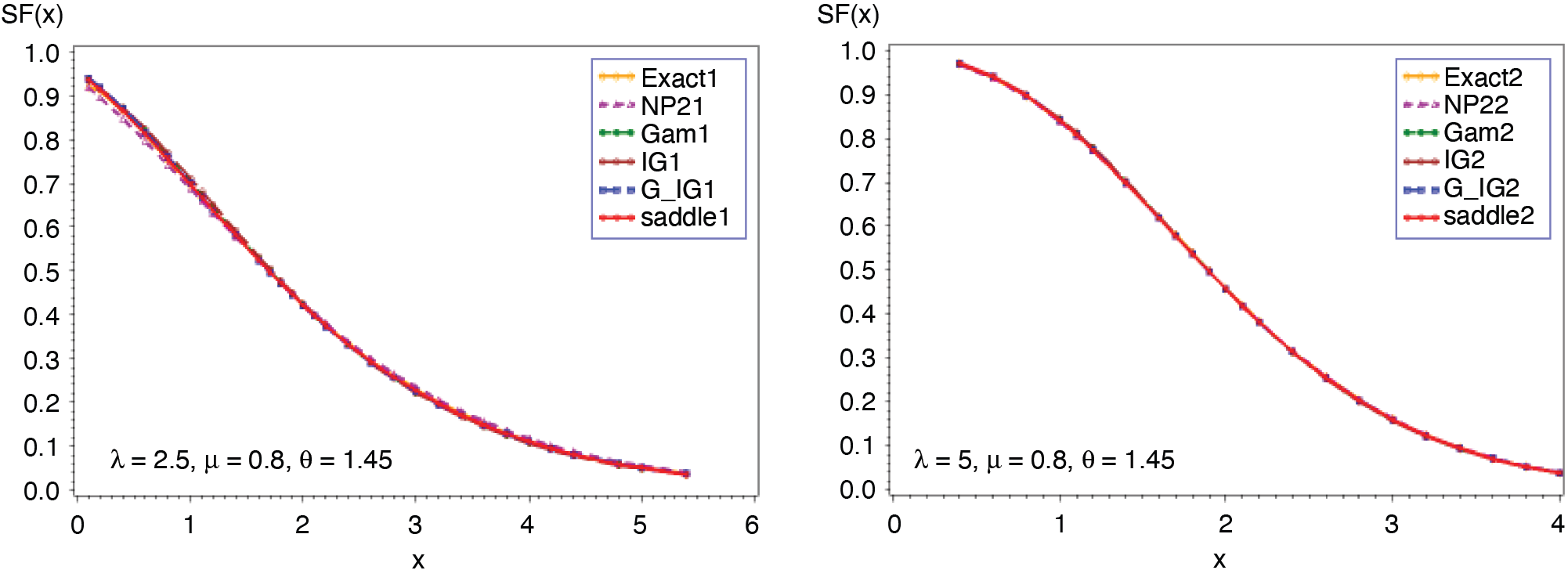
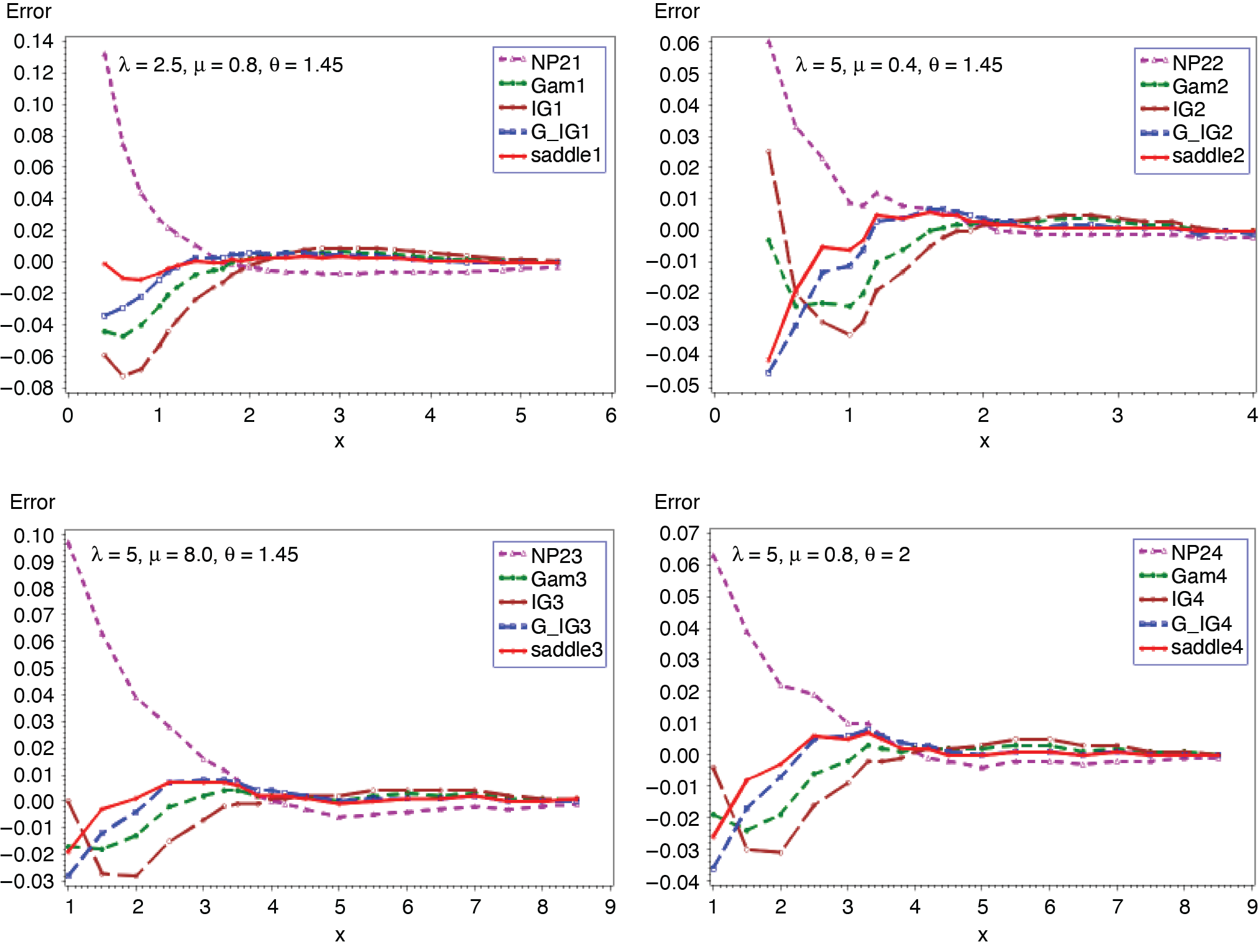
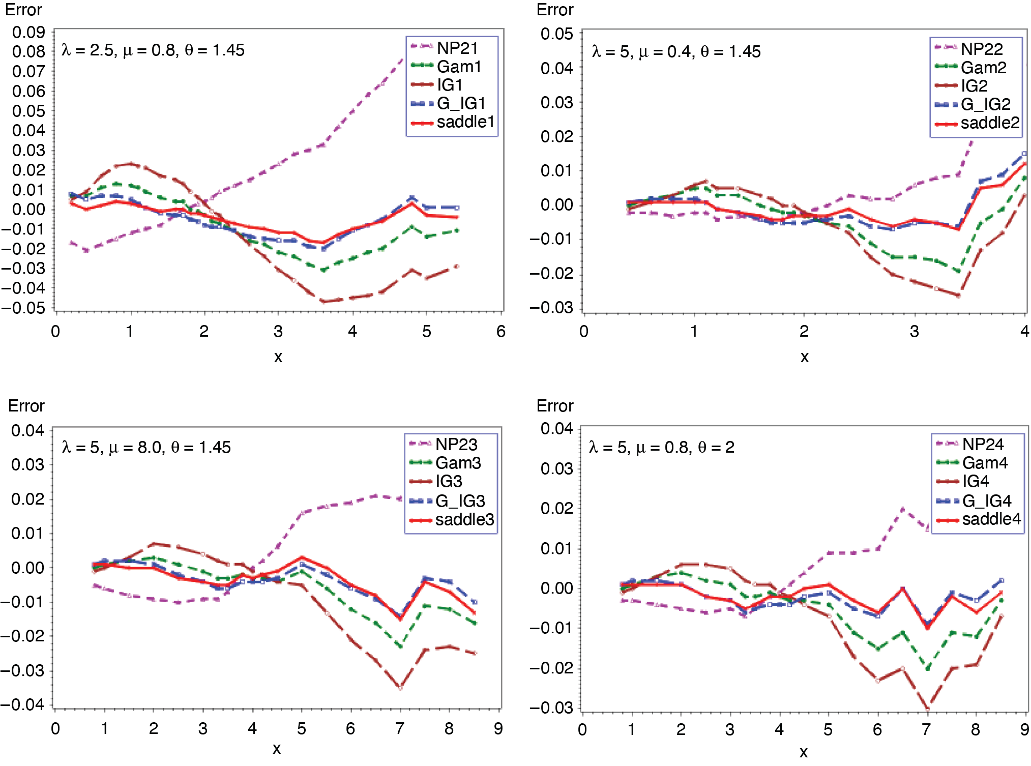
Figures 5 and 6 present the cumulative and the tail probabilities for various parameter choices of frequency and severity distributions. Figures 7 and 8 display the relative errors for those cases. The approximations given in (2.4) and (2.5) are seen to have remarkably small relative errors for all cases.

Figure 5.CF: Poisson-IG $(\lambda, \mu, \theta)$

Figure 6.SF: Poisson-IG $(\lambda, \mu, \theta)$

Figure 6.SF: Poisson-IG $(\lambda, \mu, \theta)$ (Continued)

Figure 7.CF relative error: Poisson-IG $(\lambda, \mu, \theta)$

Figure 8.SF Relative error: Poisson-IG $(\lambda, \mu, \theta)$

3.3. Binomial-gamma distribution (m, q, α, θ)

In this example, the number of claims random variable follows a binomial distribution with parameters m and q. The common severity random variable has a gamma distribution with parameters α and θ. The c.g.f. of S and its first derivative are given as

$$C_{S}(t)=m \ln \left\{1-q+q(1-\theta t)^{-\alpha}\right\}, \quad t<1 / \theta \tag{3.6}$$

$$C_{S}^{(1)}(t)=m q \alpha \theta\left[\frac{(1-\theta t)^{-\alpha-1}}{1-q+q(1-\theta t)^{-\alpha}}\right] . \tag{3.7}$$

Figure 9.CF: Binomial gamma ($m, q, \alpha, \theta$)

Figure 10.SF: Binomial gamma ($m, q, \alpha, \theta$)

Figure 10.SF: Binomial gamma ($m$, $q$, $\alpha, \theta)$ (Continued)

Figure 11.CF relative errors: binomial gamma ($m, q, \alpha, \theta$)

Figure 12.SF Relative errors: binomial gamma ($m, q, \alpha, \theta$)

The saddlepoint, $\hat{t}=\hat{t}(x)$, can be obtained numerically from

$$m q \alpha \theta\left[\frac{(1-\theta t)^{-\alpha-1}}{1-q+q(1-\theta t)^{-\alpha}}\right]=x . \tag{3.8}$$

The required moments obtained from (3.6) are as follows:

$$\begin{array}{l} \mu \mathrm{s}=m q \alpha \theta \\ \mu_{2}(\mathrm{~s})=m q \alpha[1+(1-q) \alpha] \theta^{2} \\ \mu_{3}(\mathrm{~s})=m q \alpha\left[\delta_{1}+2 \alpha^{2} q^{2}\right] \theta^{3} \\ \mu_{4}(\mathrm{~s})=m q \alpha\left[\begin{array}{c} \delta_{2}-6 \alpha^{3} q^{3} \\ +3 m q \alpha\{1+(1-q) \alpha\}^{2} \end{array}\right] \theta^{4}, \end{array}$$

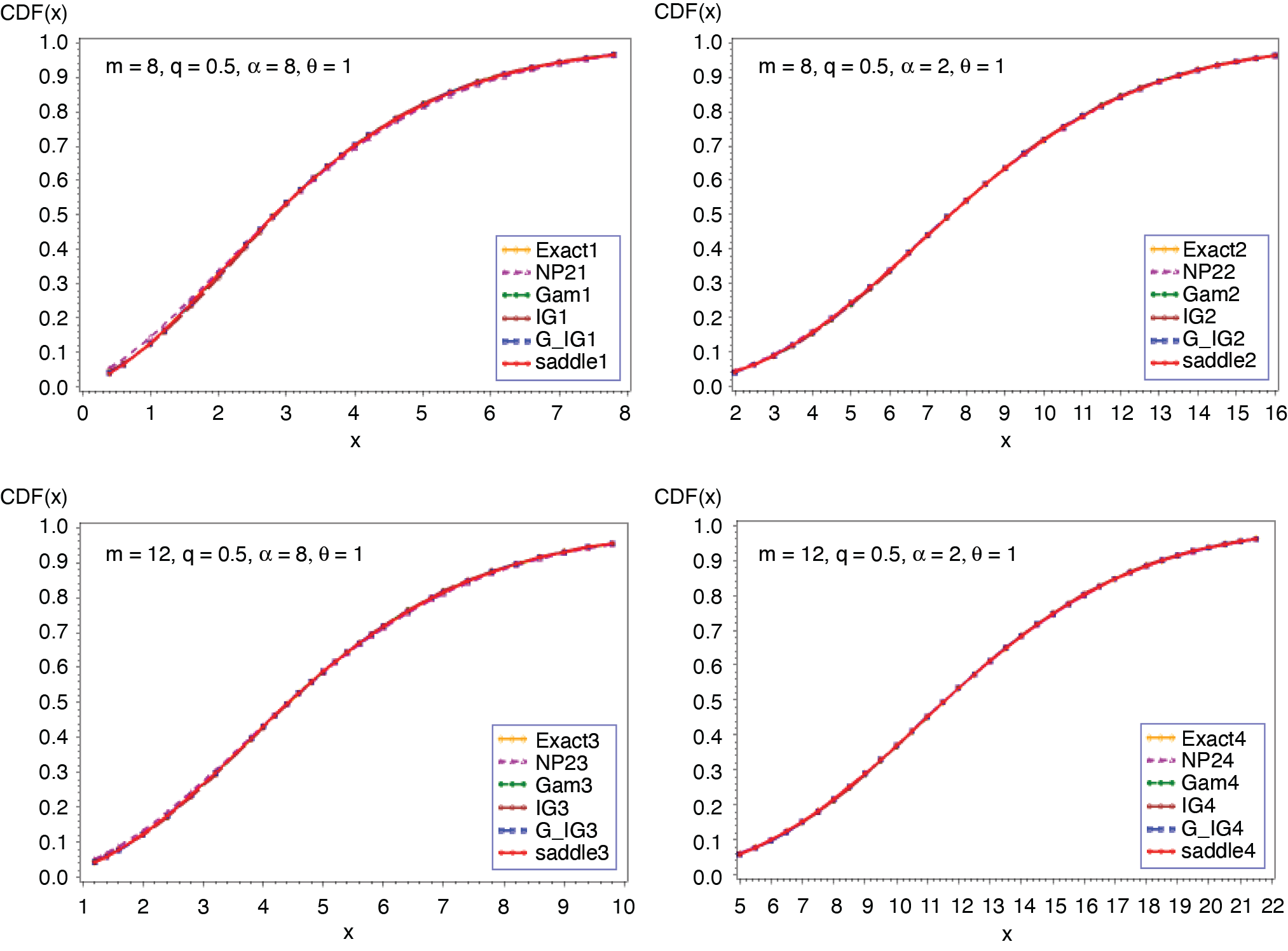
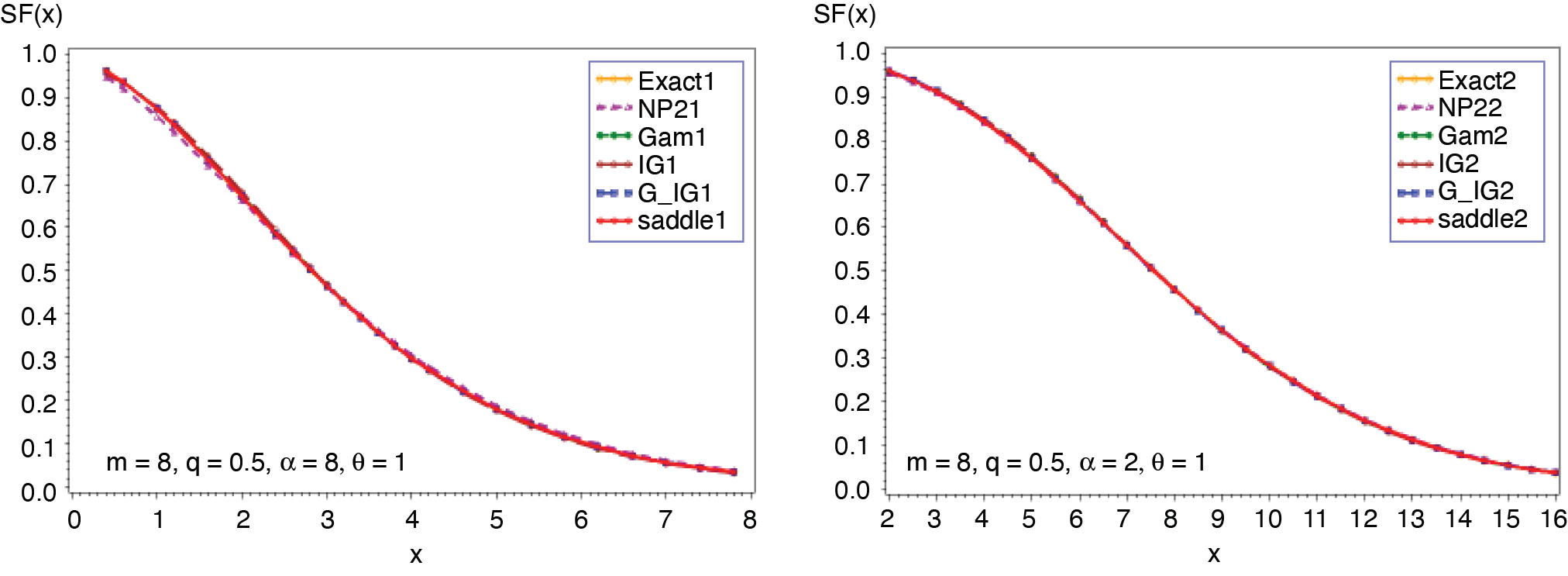
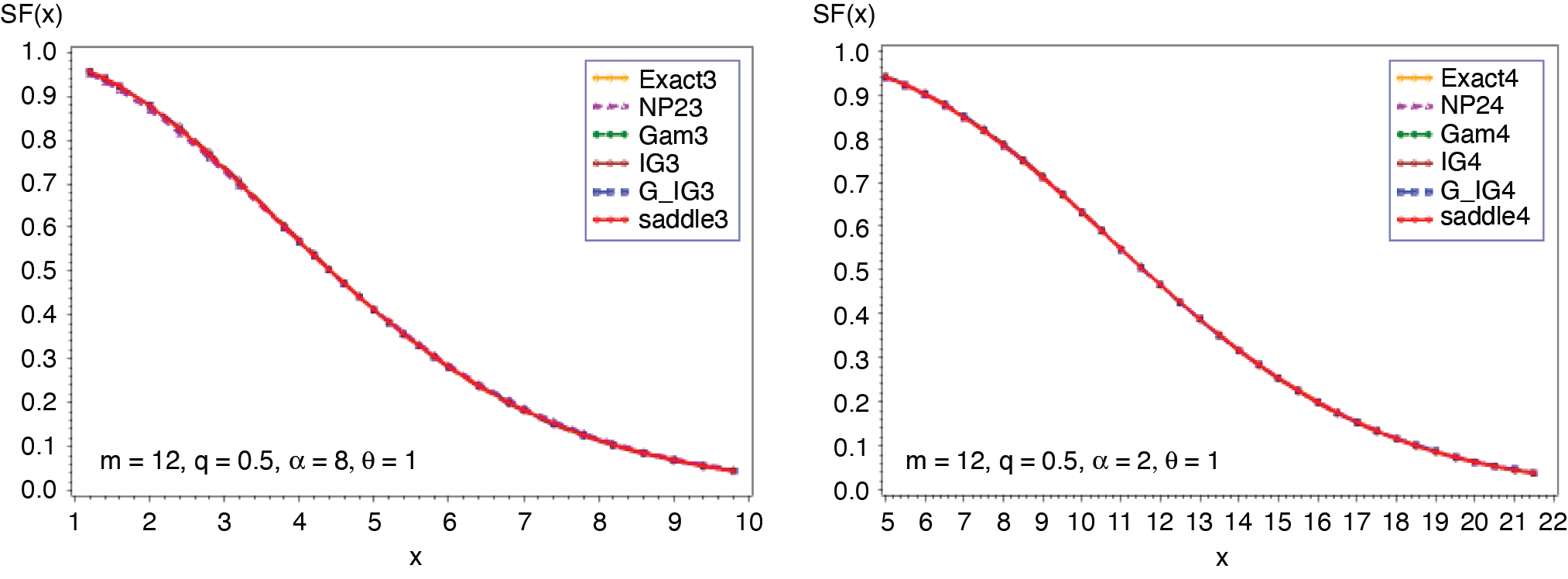
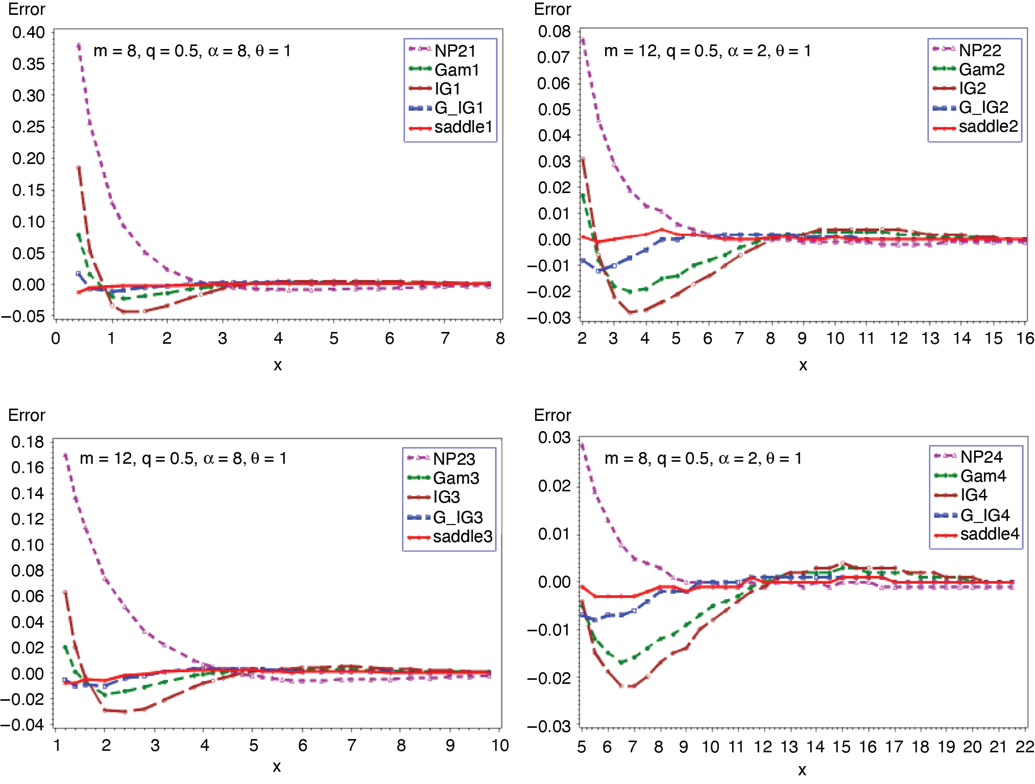
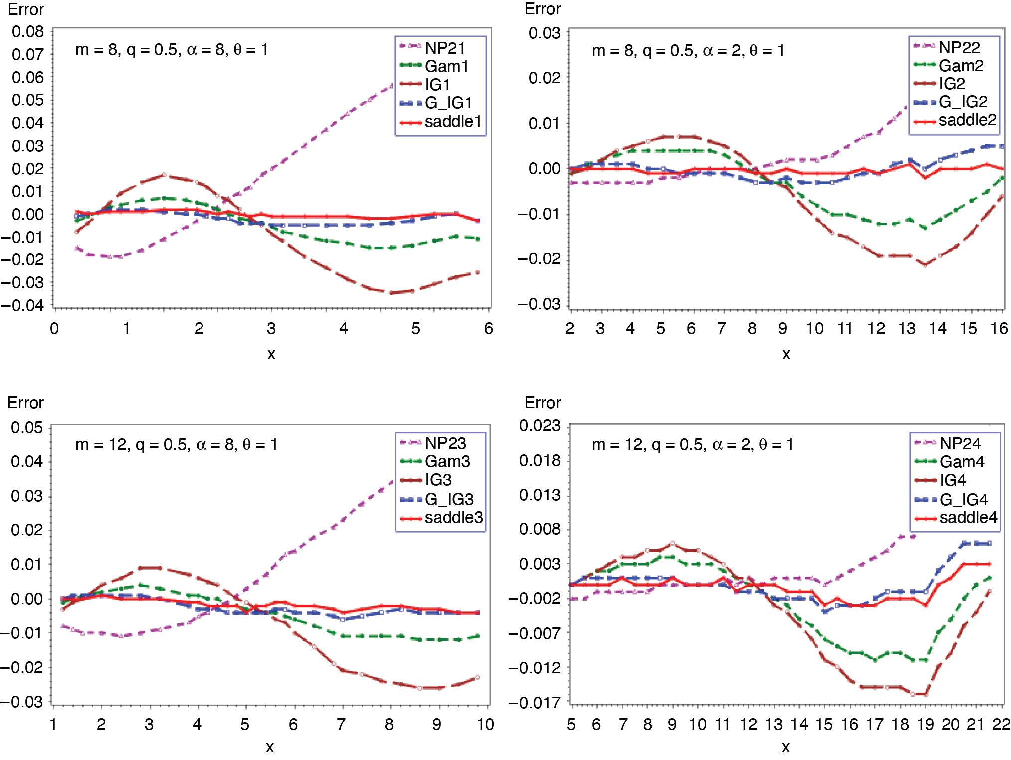
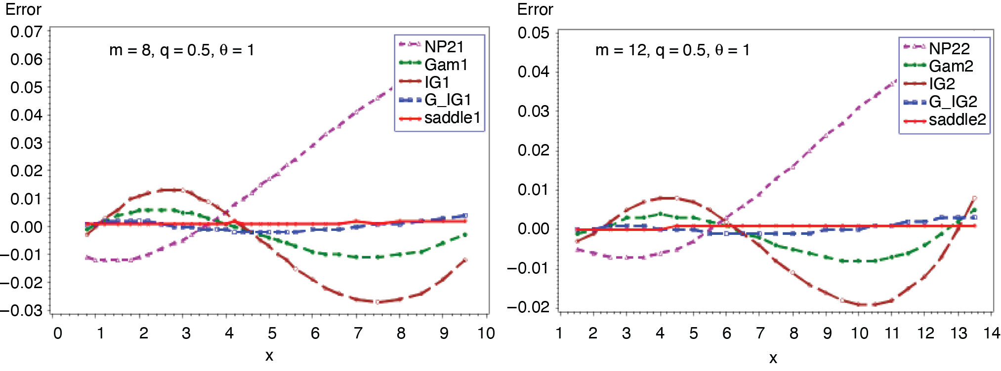
where δ₁ = (α + 1)(α + 2) − 3α(α + 1)q and δ₂ = (α + 1){(α + 2)(α + 3) − α(7α + 11)q + 12 α²q²}. Figures 9 and 10 present the cumulative and the tail probabilities for various choices of parameter values. Figures 11 and 12 depict the relative errors for those combinations. The outcomes are the same as in the previous applications. When α = 1, the above distribution modifies to binomial exponential (m, q, θ). The c.g.f. of S and its derivative reduce to

$$C_{S}(t)=\ln \left(1+\frac{q \theta t}{1-\theta t}\right)^{m}, \quad t<1 / \theta \tag{3.9}$$

$$C_{S}^{(1)}(t)=m \theta\left[\frac{1}{1-\theta t}-\frac{1-q}{1-\theta t+q \theta t}\right] . \tag{03.10}$$

The saddlepoint equation leads to the explicit solution

$$\hat{t}=\frac{(2-q)-\sqrt{q^{2}+\frac{4 m q(1-q) \theta}{x}}}{2(1-q) \theta} . \tag{3.11}$$

$$\begin{array}{l} \mu \mathrm{s}=m q \theta \\ \mu_{2}(\mathrm{~s})=m\left[1-(1-q)^{2}\right] \theta^{2} \\ \mu_{3}(\mathrm{~s})=2 m\left[1-(1-q)^{3}\right] \theta^{3} \\ \mu_{4}(\mathrm{~s})=3 m\left[2\left\{1-(1-q)^{4}\right\}+m q^{2}(2-q)^{2}\right] \theta^{4} . \end{array}$$

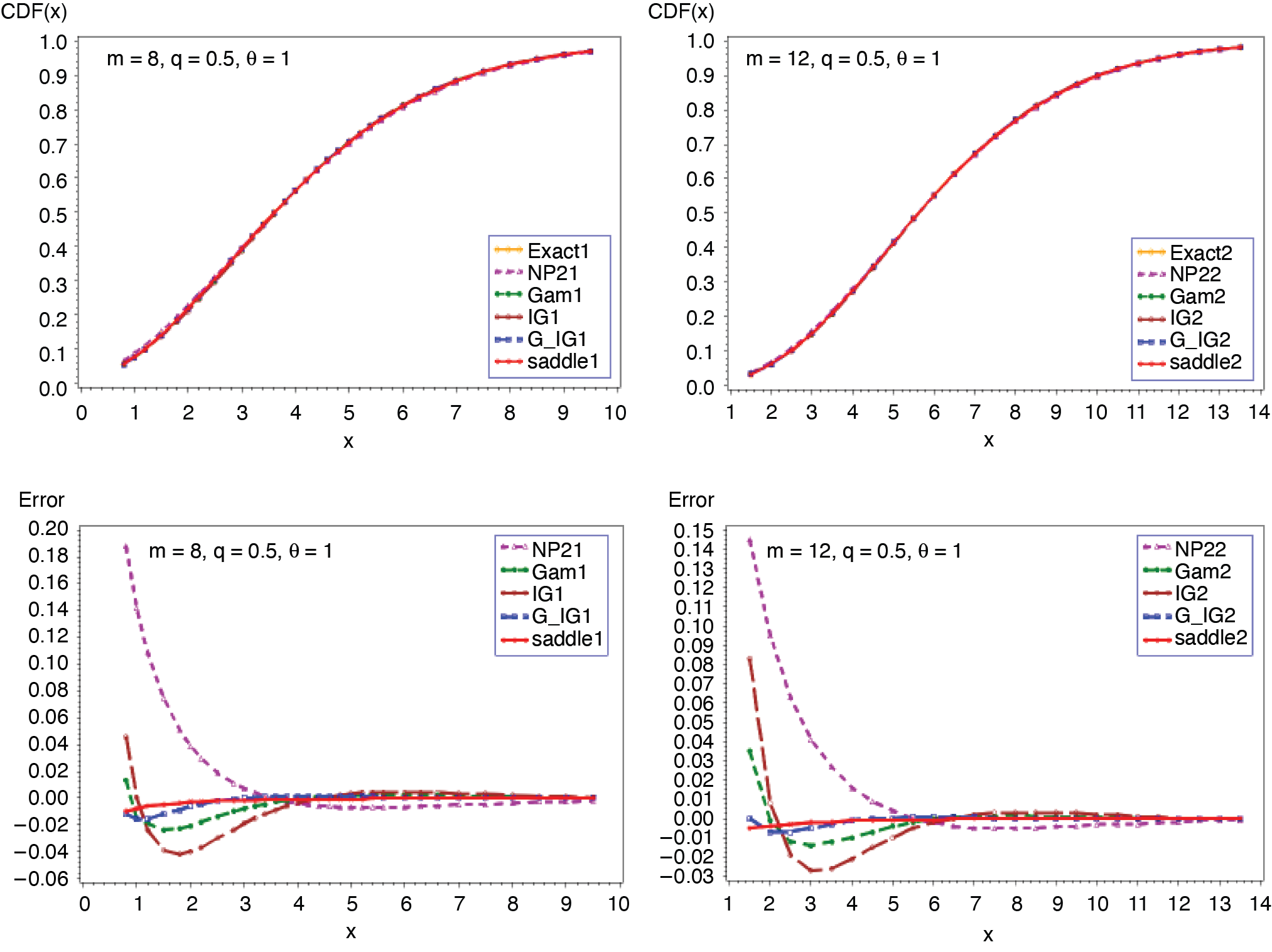
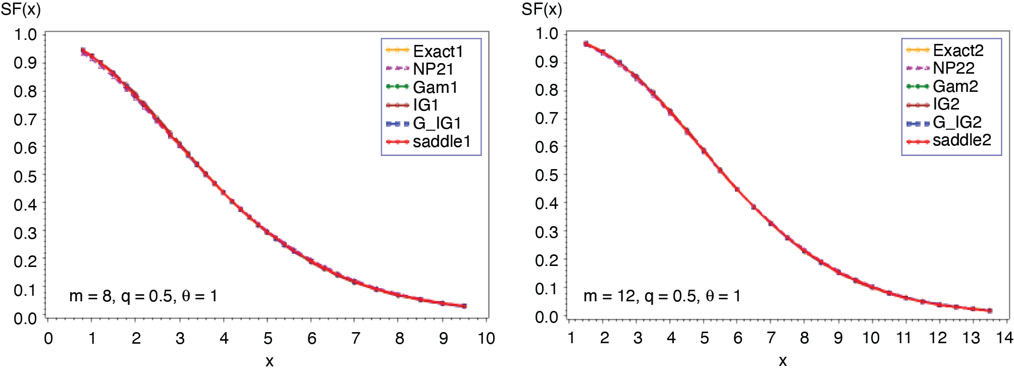
The analytical expression for the cumulative probability of S, which can easily be obtained from (1.1), is

$$C F(x)=1-\sum_{n=1}^{m}\binom{m}{n} q^{n}(1-q)^{m-n} \sum_{j=0}^{n-1} \frac{(x / \theta)^{j} \exp (-x / \theta)}{j!} . \tag{3.12}$$

Cumulative and tail probabilities, along with the relative errors of the approximations, are presented in Figures 13 and 14. The exact probabilities are obtained from (3.12). As can be seen in the previous examples, the results in Figures 13 and 14 indicate that the saddlepoint approximation gives very satisfactory accuracy.

Figure 13.CF and relative errors: binomial exponential ($m$, $q, \theta$)

Figure 14.SF and relative errors: binomial exponential ($m, q, \theta$)

Figure 14.SF and relative errors: binomial exponential ($m$, $q$, $\theta$) (Continued)

3.4. NB-exponential distribution (r, β, θ)

In this example, frequency distribution is negative binomial with parameters r and β, and the common severity distribution is exponential with parameter θ. The c.g.f. of S and its first derivative can be written as

$$C_{S}(t)=r \ln \left(\frac{1-\theta t}{1-\theta t-\beta \theta t}\right) \tag{3.13}$$

$$C_{S}^{(1)}(t)=\frac{r \beta \theta}{(1-\theta t)(1-\theta t-\beta \theta t)} . \tag{3.14}$$

Equation (3.14) yields an explicit saddlepoint solution:

$$\hat{t}=\frac{(\beta+2)-\sqrt{\beta^{2}+\frac{4 r \beta \theta(1+\beta)}{x}}}{2 \theta(1+\beta)} . \tag{3.15}$$

Equation (3.13) yields the following moments:

$$\begin{array}{l} \mu \mathrm{s}=r \beta \theta \\ \mu_{2}(\mathrm{~s})=r \beta(\beta+2) \theta^{2} \\ \mu_{3}(\mathrm{~s})=2 r\left[(1+\beta)^{3}-1\right] \theta^{3} \\ \mu_{4}(\mathrm{~s})=3 r\left[2\left\{(1+\beta)^{4}-1\right\}+r \beta^{2}(\beta+2)^{2}\right] \theta^{4} . \end{array}$$

The following analytical expression for the cumulative probability can be obtained from (1.1):

$$\begin{aligned} C F(x)= & 1-\sum_{n=1}^{r}\binom{r}{n}\left(\frac{\beta}{1+\beta}\right)^{n}\left(\frac{1}{1+\beta}\right)^{r-n} \\ & \sum_{j=0}^{n-1} \frac{(x / \theta(1+\beta))^{j} e^{-x / \theta(1+\beta)}}{j!} . \end{aligned} \tag{03.16}$$

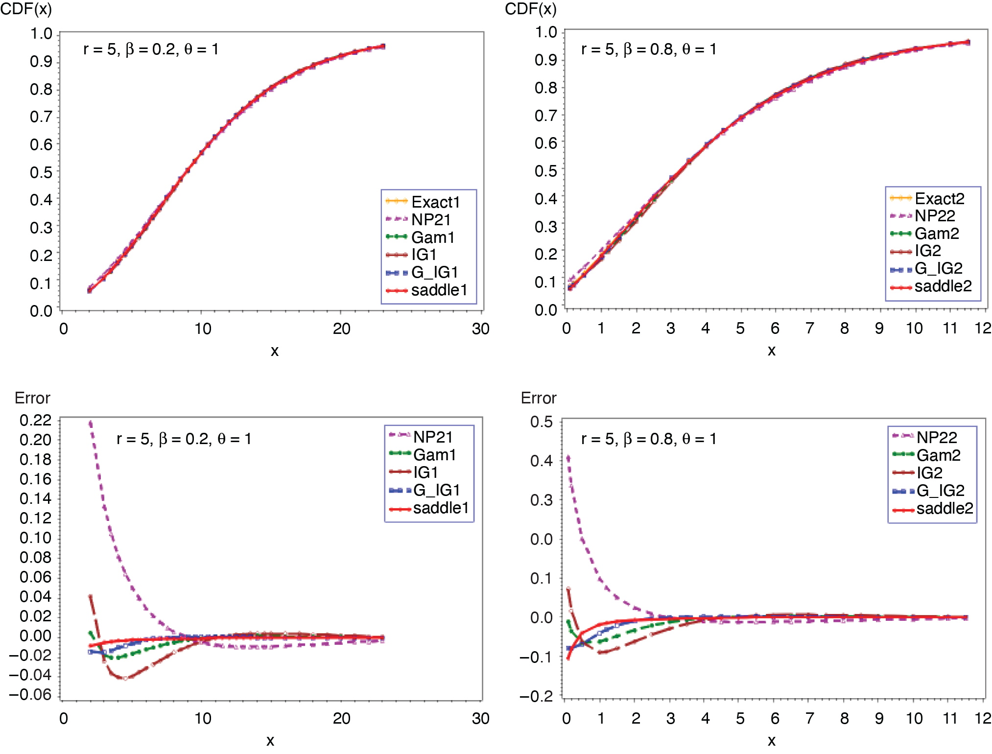
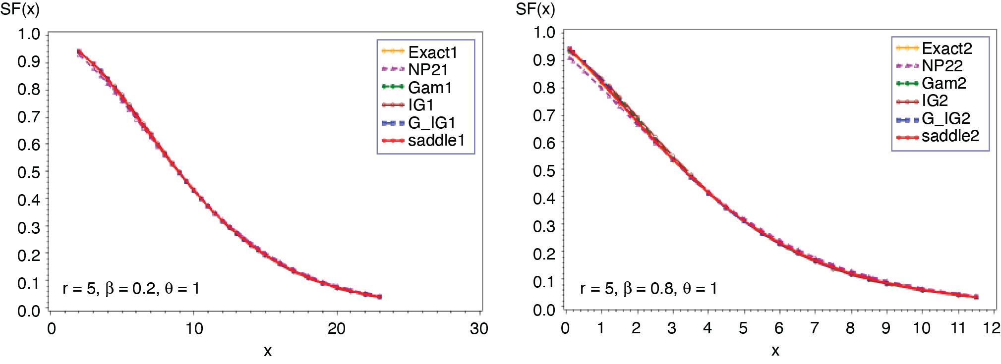
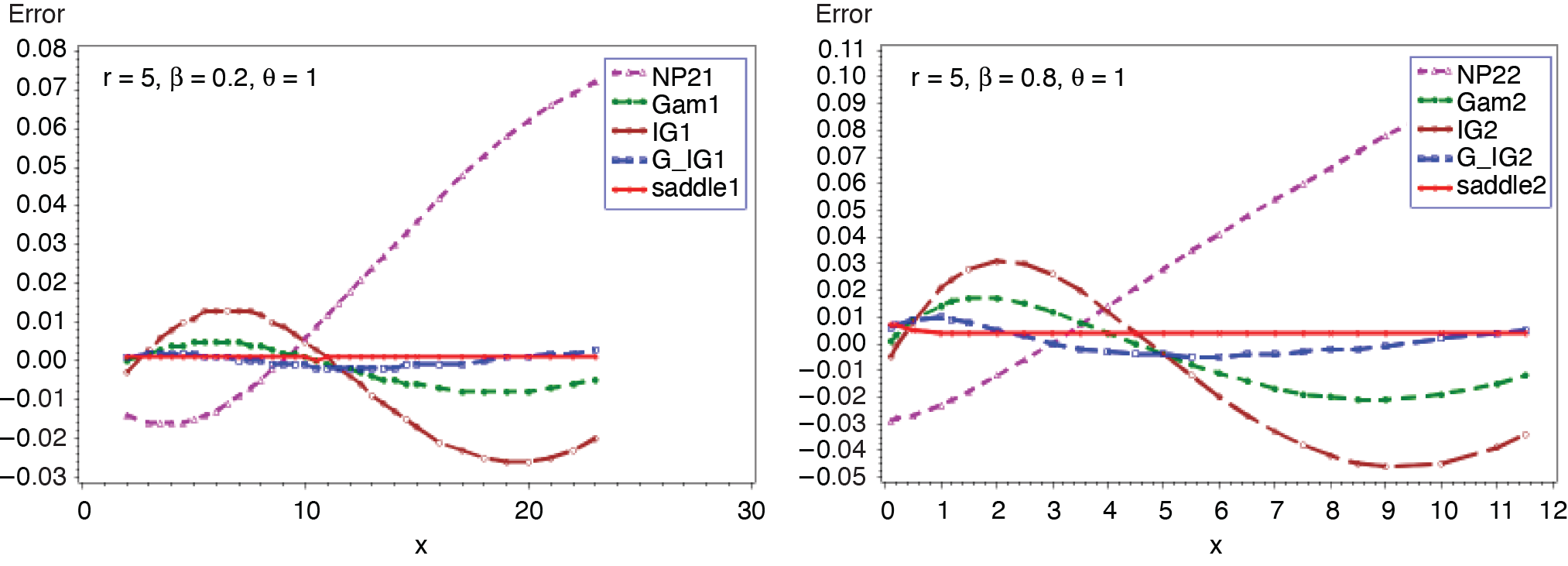
Figures 15 and 16 present the comparison of all five approximations. The exact probability is computed based on the analytical expression given in (3.16). The outcomes in Figures 15 and 16 reveal that the approximation given in (2.5) outperforms the other four, followed by the gamma-IG mixture approximation provided in (2.4). Corresponding results for geometric-exponential distribution (β, θ) can be obtained by letting r = 1.

Figure 15.CF and relative errors: NB-exponential $(r, \beta, \theta)$

Figure 16.SF and relative errors: NB-exponential $(r, \beta, \theta)$

Figure 16.SF and relative errors: NB-exponential $(r, \beta, \theta)$ (Continued)

4. Conclusions

The purpose of this paper is to compare the accuracy of the saddlepoint approximation, introduced by Lugannani and Rice (1980), with four other approximations to the distribution of aggregate claims. The approximate cumulative probabilities and tail probabilities have been computed for several compound distributions and are compared with the exact results in terms of relative errors. Based on the results in Figures 1–16, it is clear that the saddlepoint approximation gives very satisfactory accuracy, followed by the gamma-IG mixture approximation in all of the examples considered. The gamma and the IG approximations behave in a similar manner. The NP2 approximations consistently produce higher relative errors compared to the other four. Suppose claim amounts distribution is gamma or inverse Gaussian. The saddlepoint approximation is simple and easy to compute with great accuracy, requiring only the first three derivatives of the cumulant generating function.

Acknowledgment

Author would like to thank the editor and three anonymous reviewers for their constructive comments/suggestions that greatly improved the manuscript.