NCCI’s 2007 Hazard Group Mapping

undefined

1. Introduction

In the United States, most private employers are required to provide workers compensation coverage to pay employees injured on the job lost wages and medical costs arising from the work injury. Often employers provide this coverage by purchasing workers compensation insurance. For many insureds, premiums are based, in part, on the payroll classification of the employer, which is based on the type of business and operations performed by employees. For example, there is a classification for roofing businesses, and another classification for professional employees of hospitals. Currently there are about 800 different classifications in use in states for which NCCI provides ratemaking services (although the exact number used in any given state varies).

For various individual risk-rating purposes, for use in NCCI ratemaking, and for other reasons, it is useful to have tables of excess loss factors. An excess ratio or excess loss factor (ELF)^[1] is the ratio of the expected amount of claims excess of a given limit to total expected claims. Because the probability that a loss is large, given that a loss occurs, varies by class, it is useful to have ELFs that vary by class.

A hazard group is a collection of workers compensation classifications that have relatively similar expected excess loss factors over a broad range of limits. NCCI periodically publishes tables of ELFs for states where NCCI provides ratemaking services. Generally these tables are updated annually, and give ELFs (or closely related factors) by hazard group for selected limits.

At the beginning of 2007, NCCI implemented a new seven-hazard-group system, replacing the previous four-hazard-group system. That is, under the new system, each classification is assigned to one of seven hazard groups. The seven new hazard groups are not simply a subdivision of the previous four; they are a substantially different mapping of classes to hazard group. This article describes the analysis that led to the assignment of classes to the new seven hazard groups.

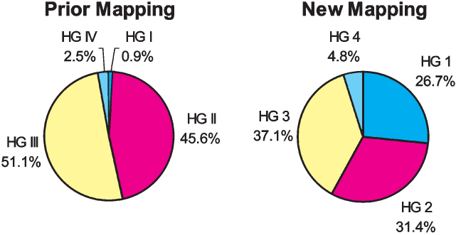
Under the previous NCCI four-hazard-group system, the bulk of workers compensation (WC) exposure in NCCI states was concentrated in two hazard groups, as can be seen in Table 1.

In our analysis, we considered whether a finer delineation would be possible, and what might be the optimal number of hazard groups. Apart from those considerations, hazard group assignments should be reviewed periodically because of changes over time in the insurance industry, technology, workplaces, and the evolution of the classification system and workers compensation infrastructure. The previous review had been done in 1993.

NCCI defines hazard groups on a country-wide basis. That is, the grouping of classes into hazard groups does not vary by state. Most workers compensation classes apply in every state where NCCI provides ratemaking services, although there are a few classes known as “state specials” that apply in only one state or a few states. NCCI takes the view, as it does in class ratemaking, that classes are homogeneous with respect to operations of the insureds, and therefore that the relative mix of injuries within a class should not vary much from state to state.

1.1. Prior work

The prior NCCI hazard groups were developed by first identifying seven variables based on relative claim frequency, severity, and pure premium, which were thought to be indicative of excess loss potential (NCCI 1993). These variables were the ratios of class average to statewide weighted average:

1. serious^[2] to total claim frequency ratio

2. serious indemnity severity^[3]

3. serious medical severity

4. serious severity, including medical

5. serious to total indemnity pure premium^[4] ratio

6. serious medical to total medical pure premium ratio

7. serious pure premium to total pure premium ratio

Because of the correlations among these seven variables, the seven variables were grouped into three subsets based on an examination of the partial correlation matrix. A principal components^[5] analysis was then done to determine a single representative variable from each of the three subsets and the linear combination of these representative variables that maximized the proportion of the total variance explained. The representative variables selected were the first, second, and last variables. The linear combination so identified is called the first principal component and is the single variable that was used to sort classes into hazard groups. Determination of the optimal number of hazard groups was outside the scope of that study and so the number of hazard groups remained unchanged at four.

A very different approach was employed by the Workers Compensation Insurance Rating Bureau of California (WCIRB 2001). The WCIRB’s objective was to group classes with similar loss distributions. They used two statistics to sort classes into hazard groups. The first statistic was the percentage of claims excess of $150,000. This statistic was thought of as a proxy for large loss potential. The second statistic measured the difference between the class loss distribution and the average loss distribution across all classes. The different hazard groups corresponded to different ranges of these two statistics. The results were checked by using cluster analysis on these two variables.

1.2. Overview

Our approach owes much to the prior work on the subject, yet it is quite distinct. We sorted classes into hazard groups based on their excess ratios rather than proxy variables. As shown in Corro and Engl (2006), a distribution is characterized by its excess ratios and so there is no loss of information in working with excess ratios rather than with the size of loss density or distribution function. Section 2 describes how we computed class-specific excess ratios.

Section 3 describes how we used cluster analysis to group classes with similar excess ratios, and how we determined that seven is the optimal number of hazard groups. In Section 4 we compare the new hazard group assignments with the prior assignments.

Following the analytic determination of hazard groups, the tentative assignments were reviewed by several underwriters, and, based on this input, NCCI changed some assignments; we describe this in Section 5.

Finally, Section 6 recaps the key ideas of this study and the key features of the new assignments.

2. Class excess ratios

Gillam (1991) describes in detail the NCCI procedure for computing excess ratios by hazard group for individual states. In the NCCI procedure, each ELF for a state and hazard group is a weighted average of ELFs by injury type specific to the state and hazard group. The ELFs for an injury type for a state and hazard group are derived from ELFs for the injury type in the state, adjusted to the estimated mean loss in the hazard group in the state. Injury types used by NCCI are Fatal, Permanent Total, Permanent Partial, Temporary Total, and Medical Only.

To put this in mathematical terms, let X_i be the random variable giving the amount of loss for injury type i in the state, and let X_i have density function f_i(x) and mean µ_i. Let S_i be the normalized state excess ratio function for injury type i; that is

\[ S_{i}(r)=E\left[\max \left(\frac{X_{i}}{\mu_{i}}-r, 0\right)\right]=\int_{r}^{\infty}(t-r) g_{i}(t) d t, \]

where g_i(x)= µ_if_i(µ_ix) is the density function of the normalized losses X_i/µ_i and r ≥ 0 can be interpreted as an entry ratio, i.e., the ratio of a loss amount to the mean loss amount. For hazard group j, the overall excess ratio R_j(L) at limit L is

\[ R_{j}(L)=\sum_{i} w_{i, j} S_{i}\left(L / \mu_{i, j}\right), \tag{1} \]

where \(w_{i, j}\) is the percentage of losses due to injury type \(i\) in hazard group \(j\) (so \(\sum_i w_{i, j}=1\) ), and \(\mu_{i, j}\) is the average cost per case for injury type \(i\) in hazard group \(j\).

In the same way we can compute countrywide excess ratios for a given class by just knowing the weights and average costs per case by injury type for a class. These excess ratios were based on the most recent five years of data, as of April 2005, and included claim counts and losses by injury type for the states where NCCI collects such data. Losses were developed, trended, and brought on-level to reflect changes in workers compensation benefits. With some minor state exceptions, the same classes apply in all states. As such, we could estimate class excess ratios on a countrywide basis. Thus for each class, c, we had a vector

\[ R_{c}=\left(R_{c}\left(L_{1}\right), R_{c}\left(L_{2}\right), \ldots, R_{c}\left(L_{n}\right)\right) \]

of excess ratios at certain loss limits L₁, L₂, . . . , L_n.

The credibility to assign to each class excess ratio vector is considered in the next subsection, and selection of the loss limits to use in the analysis is discussed in Section 3.

2.1. Credibility

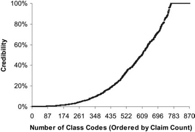
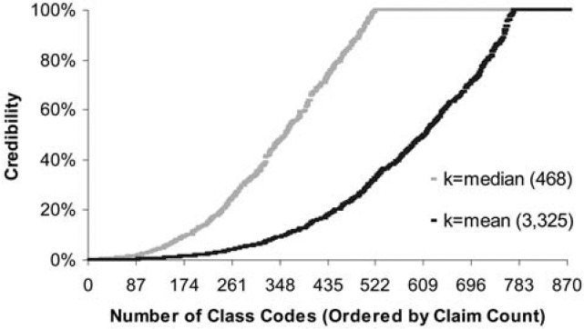
In the prior review, the credibility given to a class was

\[ z=\min \left(\frac{n}{n+k} \times 1.5,1\right), \tag{2} \]

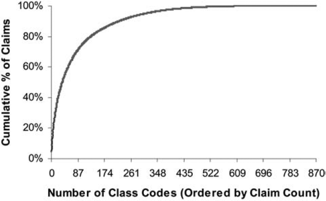
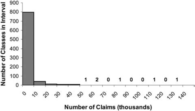
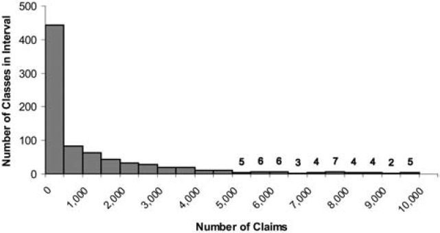
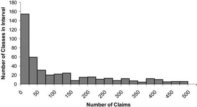
where n is the number of claims in the class and k is the average number of claims per class. This gives a class with the average number of claims 75% credibility and a class with at least twice the average number of claims full credibility. Figure 1 shows the credibility produced by this formula by size of class. The fully credible classes have over 70% of the total premium, as can be seen in Table 2. A few classes have most of the claims, as can be seen in Figure 2, where the classes with the greatest number of claims are to the left. Indeed, the distribution of claims per class is very highly skewed, as can be seen in Figure 3. Figure 4 expands the first bar in Figure 3, and shows the persistency of the skewness. And Figure 5 further expands the first bar in Figure 4, revealing the same general pattern. The average number of claims per class is nearly 10 times the median. We thus considered using the median rather than the mean for k in Formula 2. This would have resulted in a very large increase in credibility, as shown in Figure 6. We considered several other variations on Formula 2 as well. Because Medical Only claims have almost no impact on the ELFs at the published limits, we considered excluding all Medical Only claims. Taking that idea a step further, we looked at including only Serious claims. We also considered taking k in Formula 2 to be the mean number of claims over only those classes with some minimal number of claims.

In addition, we considered basing credibility on various square root rules. We considered a simple square root rule of the form

\[ z=\sqrt{\frac{n}{384}}, \]

where n is the number of claims in a class, and z is capped at 1. The full credibility standard of 384, given in Hossack, Pollard, and Zehnwirth (1983, 159), corresponds to a 95% chance of the actual number of claims being within 10% of the expected number of claims. For the determination of ELFs, serious claims (Fatal, Permanent Total, and major Permanent Partial) are more important than nonserious claims, so we looked at the following variation on the square root rule

\[ z=\frac{N_{F} \sqrt{\frac{n_{F}}{384}}+N_{M} \sqrt{\frac{n_{M}}{384}}+N_{m} \sqrt{\frac{n_{m}}{384}}}{N_{F}+N_{M}+N_{m}}, \]

where

1. n_F = the number of fatal claims in the class;

2. N_F = the number of fatal claims in all classes;

3. n_M = the number of permanent total and major permanent partial claims in the class;

4. N_M = the number of permanent total and major permanent partial claims in all classes;

5. n_m = the number of minor permanent partial and temporary total claims in the class;

6. N_m = the number of minor permanent partial and temporary total claims in all classes.

We also considered varying the full credibility standard by injury type with the following credibility formula

\[ z=\frac{N_{s} \sqrt{\frac{n_{s}}{175}}+\left(N-N_{s}\right) \sqrt{\frac{n-n_{s}}{384}}}{N} \]

where

1. n_s = the number of serious claims in the class;

2. N_s = the number of serious claims in all classes;

3. n = the total number of claims in the class;

4. N = the total number of claims in all classes.

In the end, none of the alternatives considered seemed compelling enough to warrant a change and the results did not seem to depend heavily on the credibility formula; consequently we retained Formula 2 for computing credibility.

For the complement of credibility we used the excess ratios corresponding to the current hazard group of the class. More precisely, for each class c we have a vector of excess ratios

\[ R_{c}=\left(R_{c}\left(L_{1}\right), R_{c}\left(L_{2}\right), \ldots, R_{c}\left(L_{n}\right)\right) \]

and a credibility z. We also have a vector of excess ratios for the hazard group HG containing the class c (which can be determined, as above, as a loss weighted sum over vectors for classes in HG)

\[ R_{H G}=\left(R_{H G}\left(L_{1}\right), R_{H G}\left(L_{2}\right), \ldots, R_{H G}\left(L_{n}\right)\right) . \]

We now associate to each class a credibility-weighted vector of excess ratios

\[ z R_{c}+(1-z) R_{H G} . \]

It is these credibility-weighted vectors of excess ratios that we use in the cluster analysis described in the next section.

3. Analytic determination of the new hazard groups

The fundamental analytic method used to determine the new hazard groups is Cluster Analysis. It is a way to group classes with similar ELFs and is described in this section.

3.1. Selection of loss limits

The class excess ratio is a function of the loss limit, so it was necessary to select the limits to

use in the analysis. We used limits of 100, 250, 500, 1000, and 5000, in thousands of dollars. Because excess ratios at different limits were highly correlated, five limits were thought to be sufficient. We considered using fewer limits but decided that it was better to use five limits to cover the range commonly used for retrospective rating.

We began by considering the 17 limits for which NCCI published excess loss factors before 2005. These limits, in thousands of dollars, were: 25, 30, 35, 40, 50, 75, 100, 125, 150, 175, 200, 250, 300, 500, 1000, 2000, and 5000. We modified this list by dropping $300,000 and adding $750,000. We reduced this to the five selected limits based primarily on two considerations:

• ELFs at any pair of excess limits are highly correlated across classes, especially when the ratio of the limits is close to 1.

• Limits below $100,000 are heavily represented in the list of 17 limits.

The correlations were computed using only the 162 classes with at least 75% credibility. Classes with small credibility have estimated ELFs close to those for the prior overall hazard group. Including the low-credibility classes would skew the correlations towards those of the overall hazard groups.

Even among the five selected limits, correlations between ELFs for pairs of limits are very high, as can be seen in Table 3.

Each of the 12 limits not used has a correlation coefficient of at least 0.9882 with a limit that was used, as can be seen in Table 4.

Although we ultimately used five limits, we experimented by clustering with different limits. We found that the hazard group assignments resulting from five limits were quite similar to those resulting from 17. When mapping the classes to seven hazard groups, only 68 out of 870 classes were assigned to different hazard groups and these accounted for just 5.5% of the total premium.

To see whether five limits were more than needed for the analysis, we tried clustering the classes using only a single limit. In one instance we used $100,000 and in another we used $1,000,000. Figures 7 and 8 compare those single limit assignments with clustering using the five-limit approach. In both cases, the results differed from the five-limit case, markedly so when $1,000,000 was used. This indicates that too much information is lost by dropping down to one limit. Retrospectively rated policies are purchased over a range of limits and no single limit captures the full variability in excess ratios.

We used principal components analysis to enhance the clustering investigation. The first two principal components of the five limits retained over 99% of the variation in the data. While this might suggest that fewer limits could have been used, we decided to use five limits in order to cover the range of limits commonly used in retrospective rating. The distance between two classes in principal components space does not have the same simple interpretation as it does in excess ratio space. However principal components analysis allows one to project a five-dimensional plot onto two dimensions. Clustering using the five limits and plotting the resulting hazard group assignments using the first two principal components showed that the clusters were well separated and that outliers were easily identified. In our view, this confirmed the success of the five-dimensional clustering.

3.2. Metrics

The objective of assigning classes to hazard groups is to group classes with similar vectors of excess ratios. This raises the question of how to determine how similar or “close” two vectors are. The usual approach is to measure the distance between the vectors. If

\[ x=\left(x_{1}, x_{2}, \ldots, x_{n}\right) \quad \text { and } \quad y=\left(y_{1}, y_{2}, \ldots, y_{n}\right) \]

are two vectors in \(\mathbb{R}^n\), then the usual Euclidean, or \(L^2\), distance between \(x\) and \(y\) is specified as

\[ \|x-y\|_{2}=\sqrt{\sum_{i=1}^{n}\left(x_{i}-y_{i}\right)^{2}} . \]

This metric is used extensively in statistics and is what we used. In linear regression this metric penalizes large deviations. That is, one big deviation is seen to be worse than many small deviations.

There are many other metrics. Perhaps the second most common distance function is the L¹ metric which specifies

\[ \|x-y\|_{1}=\sum_{i=1}^{n}\left|x_{i}-y_{i}\right|. \]

Here a large deviation in one component gets no more weight than many small deviations. The intuitive rationale for using this metric is that it minimizes the relative error in estimating excess premium. If R_c(L) is the hypothetically correct excess ratio at a limit of L for a class c and the premium on the policy is P then the excess premium is given by P · PLR · R_c(L), where PLR denotes the permissible loss ratio. But in practice the class excess ratio is approximated by the hazard group excess ratio R_HG(L). The relative error in estimating the excess premium is then

\[ \begin{array}{c} \frac{\left|P \cdot P L R \cdot R_{H G}(L)-P \cdot P L R \cdot R_{c}(L)\right|}{P} \\ =P L R \cdot\left|R_{H G}(L)-R_{c}(L)\right| . \end{array} \]

If we assume that each loss limit is equally likely to be chosen by the insured, then the expected relative error in estimating the excess premium is given by

\[ \sum_{i=1}^{n} \frac{P L R}{n}\left|R_{H G}\left(L_{i}\right)-R_{c}\left(L_{i}\right)\right|=\frac{P L R}{n}\left\|R_{H G}-R_{c}\right\|_{1}, \]

which is proportional to the L¹ distance between the two excess ratio vectors.

Our analysis was not very sensitive to whether the L¹ or L² metric was used and we preferred the more traditional L² metric.

3.3. Standardization

When clustering variables are measured in different units, standardization is typically applied to prevent a variable with large values from exerting undue influence on the results. Standardization ensures that each variable has a similar impact on the clusters. Duda and Hart (1973) point out that standardization is appropriate when the spread of values in the data is due to normal random variation, however “it can be quite inappropriate if the spread is due to the presence of subclasses. Thus, this routine normalization may be less than helpful in the cases of greatest interest.”

We considered two common approaches to standardization. The usual approach is to subtract the mean and divide by the standard deviation of each variable. For example, if x₁, x₂, . . . , x_n are the sample values of some random variable, with sample mean x, and sample standard deviation s, then the standardized values are given by

\[ z_{i}=\frac{x_{i}-\bar{x}}{s}. \]

An alternative standardization method depends on the range of observations. Under this approach we would take

\[ z_{i}=\frac{x_{i}-\min x_{i}}{\max x_{i}-\min x_{i}} . \]

We conducted two cluster analysis trials in which we standardized according to the approaches described above. In each case we clustered the classes into seven hazard groups. Both trials resulted in hazard groups that were not very different from those produced without standardization.

Further, two issues were apparent with regard to standardizing in our particular analysis. First, excess ratios at different limits have a similar unit of measure, which is dollars of excess loss per dollar of total loss. That is, excess ratios share a common denominator. Any attempt to standardize would have resulted in new variables without a common unit interpretation. Second, all excess ratios are between zero and one. Some standardization approaches would have resulted in standardized observations outside this range.

Another consideration is the greater range of excess ratios at lower limits. Without standardization, the excess ratios at lower loss limits have more influence on the clusters than do those at higher limits. This result is not undesirable because excess ratios at lower limits are based more on observed loss experience than on fitted loss distributions (see Corro and Engl 2006). Even on a nationwide basis, there are few claims with reported losses above $5,000,000, but there are many more claims above $100,000. Greater confidence can be placed in the relative accuracy of excess ratios at lower limits because they are based on a greater volume of data.

In summary, the determination was made not to standardize because standardization would have eliminated the common denominator and it would have led to increased emphasis on higher limits. Our clustering algorithm used the L² metric and unstandardized credibility-weighted class excess ratios at the five selected loss limits: $100,000, $250,000, $500,000, $1,000,000, and $5,000,000. Premium weights were used to cluster the classes, as will be discussed in the next section.

3.4. Cluster analysis

Given a set of n objects, the objective of cluster analysis is to group similar objects. In our case, we wanted to group classes with similar vectors of excess ratios, where similarity is determined by the L² metric. At this stage the number of clusters is taken as given. Typically partitions of the objects into 1, 2, 3, . . . , n clusters are considered. Non-hierarchical cluster analysis simply seeks the best partition for any given number of clusters. In hierarchical cluster analysis the partition with k + 1 clusters is related to the partition with k clusters in that one of the k clusters is simply subdivided to get the k + 1 element partition. Thus if two objects are in different clusters in the k cluster partition then they will be in different clusters in all partitions with more than k elements. This places a restriction on the clusters that can be sensible in some contexts. Our approach was non-hierarchical.

3.5. Optimality of k-means

The clustering technique we used is called k-means. For a given number, k, of clusters, k-means groups the classes into k hazard groups so as to minimize

\[ \sum_{i=1}^{k} \sum_{c \in H G_{i}}\left\|R_{c}-\bar{R}_{i}\right\|_{2}^{2}, \tag{3} \]

where the centroid

\[ \bar{R}_{i}=\frac{1}{\left|H G_{i}\right|} \sum_{c \in H G_{i}} R_{c} \]

is the average excess ratio vector for the \(i\) th hazard group and \(\left|H G_i\right|\) denotes the number of classes in hazard group \(i\). Theoretically there is a difference between the hazard group excess ratio vector, \(R_{H G_i}\), computed using (1), and the hazard group centroid, \(\bar{R}_i\), but in practice this difference is very small.

There is a commonly used algorithm to determine clusters, known as the k-means algorithm (Johnson and Wichern 2002). To start, some assignment to clusters is made. The algorithm then has two steps, performed iteratively until the clustering stabilizes. The first step is to compute the centroid of each cluster. The second step is to find the centroid closest to each class, and assign the class to that cluster. If any classes have been reassigned from one cluster to another during the second step, return to the first step. If no classes have been reassigned, then the algorithm terminates.

Commercial software for clustering is also available. We computed clusters using the SAS FASTCLUS routine.^[6]

Hazard groups determined by k-means have several desirable optimality properties. First, they maximize the following statistic

\[ 1-\frac{\sum_{i=1}^{k} \sum_{c \in H G_{i}}\left\|R_{c}-\bar{R}_{i}\right\|_{2}^{2}}{\sum_{c}\left\|R_{c}-\bar{R}\right\|_{2}^{2}}, \tag{4} \]

where

\[ \bar{R}=\frac{1}{C} \sum_{c} R_{c} \]

is the overall average excess ratio vector, with C = Σ|HG_i| being the total number of classes. Formula (4) is analogous to the R² statistic in linear regression. It gives the percentage of the total variation explained by the hazard groups.

A second way to evaluate hazard groups is based on the traditional concepts of within and between variance. We would like the hazard groups to be homogeneous and well separated. Thus we would like to minimize the within variance and maximize the between variance; using k-means accomplishes both.

Instead of considering a single excess ratio for each class, we have a vector of excess ratios, one excess ratio for each of several fixed loss limits. Thus we do not have a single random variable corresponding to an excess ratio at a single loss limit, but rather a random vector, with one random variable, the excess ratio, for each loss limit, from which we get a variance-covariance matrix. If X_i is the random variable for the excess ratio function at the ith loss limit, L_i, across classes c, then the observed values are the R_c(L_i). The variance-covariance matrix of the random vector X = (X₁, X₂, . . . , X_n) is given by

\[ \Sigma=\left[\begin{array}{cccc} \sigma_{11} & \sigma_{12} & \cdots & \sigma_{1 n} \\ \sigma_{21} & \sigma_{22} & \cdots & \sigma_{2 n} \\ \vdots & \vdots & \ddots & \vdots \\ \sigma_{n 1} & \sigma_{n 2} & \cdots & \sigma_{n n} \end{array}\right], \]

where

\[ \sigma_{i k}=E\left[\left(X_{i}-\mu_{i}\right)\left(X_{k}-\mu_{k}\right)\right] \]

is the covariance of X_i and X_k and µ_i = E[X_i]. If we regard X as a 1 × n matrix then

\[ \Sigma=E\left[(X-\mu)^{T}(X-\mu)\right], \]

where \(\mu=\left(\mu_1, \mu_2, \ldots, \mu_n\right)\) and \((X-\mu)^T\) is the transpose of \((X-\mu)\).

In practice the variance-covariance matrix is not known, but must be estimated from the data, i.e., the vectors

\[ R_{c}=\left(R_{c}\left(L_{1}\right), R_{c}\left(L_{2}\right), \ldots, R_{c}\left(L_{n}\right)\right) . \]

Let

\[ \bar{x}_{j}=\frac{1}{C} \sum_{c} R_{c}\left(L_{j}\right), \]

where C is the total number of classes, and let

\[ \bar{x}=\left(\bar{x}_{1}, \bar{x}_{2}, \ldots, \bar{x}_{n}\right) . \]

Then the sample covariance of the ELFs at L_i and L_k is

\[ s_{i k}=\frac{1}{C} \sum_{c}\left(R_{c}\left(L_{i}\right)-\bar{x}_{i}\right)\left(R_{c}\left(L_{k}\right)-\bar{x}_{k}\right), \]

and the sample variance-covariance matrix is given by

\[ \begin{aligned} S & =\left[\begin{array}{cccc} s_{11} & s_{12} & \cdots & s_{1 n} \\ s_{21} & s_{22} & \cdots & s_{2 n} \\ \vdots & \vdots & \ddots & \vdots \\ s_{n 1} & s_{n 2} & \cdots & s_{n n} \end{array}\right] \\ & =\frac{1}{C} \sum_{c}\left(R_{c}-\bar{x}\right)^{T}\left(R_{c}-\bar{x}\right) . \end{aligned} \]

One way to generalize the concept of variance to the multivariate context is to consider the trace of S, the sum of the main diagonal of S

\[ \operatorname{trace}(S)=s_{11}+s_{22}+\cdots+s_{n n} . \]

This is just the sum of the sample variances of each variable and is called the total sample variance.

We let

\[ T=C S=\sum_{c}\left(R_{c}-\bar{x}\right)^{T}\left(R_{c}-\bar{x}\right) . \]

The matrix T is proportional to the variance-covariance matrix for the whole data set. It is called the dispersion matrix, and is the matrix of sums of squares and cross products. We can proceed similarly within each hazard group and define

\[ W_{i}=\sum_{c \in H G_{i}}\left(R_{c}-\bar{x}_{i}\right)^{T}\left(R_{c}-\bar{x}_{i}\right) . \]

If we let

\[ B_{i}=\left|H G_{i}\right|\left(\bar{x}_{i}-\bar{x}\right)^{T}\left(\bar{x}_{i}-\bar{x}\right), \]

then it can be shown (see Späth 1985) that

\[ \sum_{c \in H G_{i}}\left(R_{c}-\bar{x}\right)^{T}\left(R_{c}-\bar{x}\right)=B_{i}+W_{i} . \]

We then let

\[ W=\sum_{i=1}^{k} W_{i}. \]

This is the pooled within group dispersion matrix. For the between variance we let

\[ B=\sum_{i=1}^{k} B_{i} . \]

This is the weighted between group dispersion matrix. We then have

\[ T=B+W. \]

This means, roughly that the total variance is the sum of the between variance and the within variance. Taking the trace we get

\[ \operatorname{trace}(T)=\operatorname{trace}(B)+\operatorname{trace}(W). \]

Thus the total sample variance is the sum of the between and within sample variance. Because trace(T) is constant, maximizing trace(B) is equivalent to minimizing trace(W), which is what k-means cluster analysis accomplishes.

3.6. Weighted k-means

As observed in Section 2, some classes are much larger than others. To avoid letting the small classes have an undue influence on the analysis, we weighted each class by its premium. In simplest terms, this amounts to counting a class twice if it has twice as much premium as the smallest class. So instead of minimizing the expression in (3), we instead minimized

\[ \sum_{i=1}^{k} \sum_{c \in H G_{i}} w_{c}\left\|R_{c}-\bar{R}_{i}\right\|_{2}^{2}, \]

where w_c is the percentage of the total premium in class c. We used the premium-weighted centroids as well, that is

\[ \bar{R}_{i}=\frac{\sum_{c \in H G_{i}} w_{c} R_{c}}{\sum_{c \in H G_{i}} w_{c}} . \]

3.7. Optimal number of hazard groups

So far, we have discussed the task of determining clusters when the number of clusters is given. We now address how to tell whether one number of clusters performs better than another, e.g., whether seven clusters works better than six or eight.

Various test statistics can be used to help determine the optimal number of clusters. The procedure is to compute the test statistic for each number of clusters under consideration and then identify the number of clusters at which the chosen statistic reaches an optimal value (either a minimum or a maximum, depending on the particular test statistic being used). Milligan and Cooper (1985) and Cooper and Milligan (1988) tested such procedures to determine which statistics were the most reliable.

Milligan and Cooper (1985) performed a simulation to test 30 procedures. The simulated clusters were well separated from each other and they did not overlap. For each simulated data set, the true number of clusters was known, and they computed the number of clusters indicated by each method of determining the optimal number of clusters. The methods were ranked according to the number of times that they successfully indicated the correct number of clusters.

They noted that their simulation was idealized but that “It is hard to believe that a method that fails on the present data would perform better on less defined structures” (1985, p. 161). Hence, although the hazard group data had both noise and overlap, it was useful to refer to Milligan and Cooper (1985) to determine which methods to rule out.

In a later study, Cooper and Milligan (1988) conducted tests that were more relevant to our application because random errors were added to the simulated data. That study found that the two best performing methods in the error-free scenario were also the best with errors (Cooper and Milligan 1988, 319). The best performing method is due to Calinski and Harabasz. Milligan and Cooper (1985, 163) define the Calinski and Harabasz statistic as

\[ \frac{\operatorname{trace}(B) /(k-1)}{\operatorname{trace}(W) /(n-k)} \]

where n is the number of classes and k is the number of hazard groups, B is the between cluster sum of squares and cross product matrix, and W is the within cluster sum of squares and cross product matrix. Higher values of this statistic indicate better clusters because that corresponds to higher between clusters distances (the numerator) and lower within cluster distances (the denominator). This test is also known as the Pseudo-F test due to its resemblance to the F-test of regression analysis, often used to determine whether the explanatory variables as a group are statistically significant.

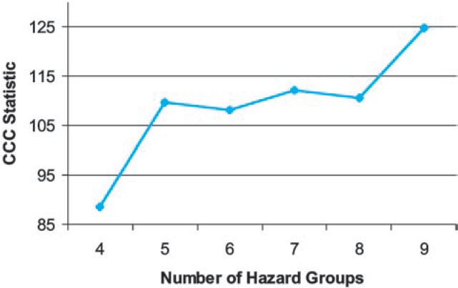
Another test that ranked high in the Milligan and Cooper testing was the Cubic Clustering Criterion (CCC). This test compares the amount of variance explained by a given set of clusters to that expected when clusters are formed at random based on data sampled from the multidimensional uniform distribution. If the amount of variance explained by the clusters is significantly higher than expected then a high value of the CCC statistic will result, indicating a high-performing set of clusters. An optimum number of clusters is identified when the test statistic reaches a maximum (Milligan and Cooper 1985, 164).

Milligan and Cooper (1985) found that the Calinski and Harabasz test produced the correct number of clusters for 390 data sets out of 432. The CCC test produced the correct value 321 times. We could not use some of the other methods that ranked high because they were only applicable to hierarchical clustering, or for other reasons.

In a SAS Institute technical report, Sarle (1983) noted that the CCC is less reliable when the data is elongated (i.e., variables are highly correlated). Excess ratios are correlated across limits, so we gave the CCC results less weight than the Calinski and Harabasz results.

We performed cluster analyses for four to nine hazard groups. There were four hazard groups in the prior NCCI system, and we saw no reason to consider any smaller number. Implementing 10 or more hazard groups would be substantially more difficult than implementing nine or fewer, because having 10 or more requires an additional digit for coding hazard groups. Testing up to nine was appropriate because the Workers Compensation Insurance Rating Bureau of California uses nine hazard groups (WCIRBC 2001).

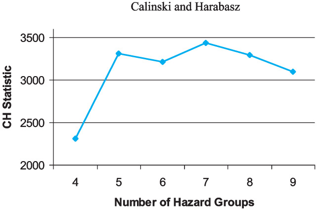
In the first phase of our cluster analysis, we assigned classes and calculated the two test statistics for each number of groups under consideration. Figure 9 shows that the Calinski and Harabasz statistic indicated that the best number of hazard groups was seven. Figure 10 shows that the CCC statistic suggested nine hazard groups.

But nine hazard groups produced crossover, meaning that at some high loss limit the hazard group excess ratio for a higher hazard group was lower than the hazard group excess ratio for a lower hazard group. While crossover is possible in principle (from a purely mathematical standpoint, it is easy to specify two loss distributions so that one has higher ELFS at low limits and the other has higher ELFs at high limits), we don’t think the data provided strong evidence for crossover, and one of our guiding principles was that there would be no crossover in the final hazard groups. In our opinion, the crossover that occurred with the clustering into nine hazard groups suggested that nine is more clusters than can accurately be distinguished.

As can be seen in Table 2, most of the premium is concentrated in the largest classes with the highest credibility. We were concerned that the indicated number of hazard groups in the analysis could have been distorted by the presence of hundreds of non-credible classes. In the second phase of our cluster analysis, we applied the tests to determine the optimal number of clusters using large classes only.

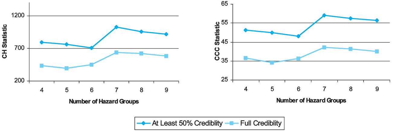
In one scenario, we applied the Calinski and Harabasz and CCC tests using only those classes with credibility greater than or equal to 50 percent. In a second scenario, we applied the tests using only fully credible classes. As shown in Figure 11, the indicated number of hazard groups was seven for both tests in both scenarios.

In summary, we used two test statistics in three scenarios for a total of six tests. Seven hazard groups was the indicated optimal number in five of these six tests. The exception was the scenario in which all classes were included, where the CCC test indicated that nine hazard groups were optimal. There are four reasons why this exception received little emphasis:

• Milligan and Cooper (1985) and Cooper and Milligan (1988) found that the Calinski and Harabasz procedure outperformed the CCC procedure.

• The CCC procedure deserves less weight when correlation is present, which was the case in all of our scenarios.

• The selection of the optimal number of clusters ought to be driven by the large classes where most of the experience is concentrated. The large classes have the highest credibility and so the most confidence can be placed in their excess ratios.

• There is crossover in the nine hazard groups, and we had a guiding principle that there would not be crossover.

We concluded that seven hazard groups were optimal. These are denoted A to G, with Hazard Group A having the smallest ELFs and Hazard Group G having the largest.

3.8. Alternate mapping to four hazard groups

We recognized that some insurers would not be able to adopt the seven hazard group system immediately because they needed additional time to make the necessary systems changes. Therefore we produced a four hazard group alternative to supplement the seven hazard group system. We chose to collapse the seven hazard groups into four by combining Hazard Groups A and B to form Hazard Group 1, combining C and D to form 2, combining E and F to form 3, and letting Hazard Group 4 be the same as G. Having an alternate mapping to four hazard groups simplifies comparisons between the prior and new mappings as well.

Prior to choosing this simple scheme we considered other alternatives. We tried using k-means cluster analysis to map the seven hazard group centroids into four. This approach resulted in a hazard group premium distribution that was not homogeneous enough. Another approach we considered was using cluster analysis to group the classes directly into four hazard groups. That approach yielded reasonable results, but it resulted in a non-hierarchical collapsing scheme, i.e., the seven hazard groups were not a result of subdividing the four hazard groups. The hierarchical collapsing scheme we chose has this feature, which allows users to know which of the four hazard groups a class is in based on knowing that class’ assignment in the seven hazard group system.

The new four hazard group system is intended to be temporary. The four hazard group system is in place only to ensure that all carriers have sufficient time to make the transition to seven hazard groups.

4. Comparison of new mapping with old

4.1. Distribution of classes and premium

The bulk of the exposure was concentrated in two of the hazard groups prior to our review. Hazard Groups I and IV contained a small percentage of the total premium. Hazard Groups II and III, on the other hand, contained 97 percent of the total premium (see Table 1). We knew that a more homogeneous distribution of premium by hazard group would improve pricing accuracy. When discussing the new hazard groups in this section we will focus on the mapping that resulted directly from the statistical analysis. Later on, as will be discussed in the underwriting review subsection, numerous classes were reassigned among the groups based on feedback gathered in our survey of underwriting experts. These changes are not reflected in Figures 12 to 20.

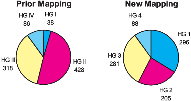
Figures 12 and 13 compare the prior mapping to the collapsed new mapping based on the distribution of classes and premium. Hazard Group 1 has a large number of classes and a substantial portion of total premium in contrast to Hazard Group I. Hazard Groups 2 and 3 have become slightly smaller than before although they are still large. In the prior mapping Hazard Groups II and III each had over 45 percent of the premium, but in the new mapping, none of the four groups has as much as 40 percent. This refinement allows for improved homogeneity of classes within each hazard group. Hazard Group 4 has retained a similar number of classes but it has more premium than Group IV.

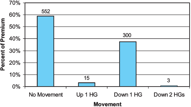
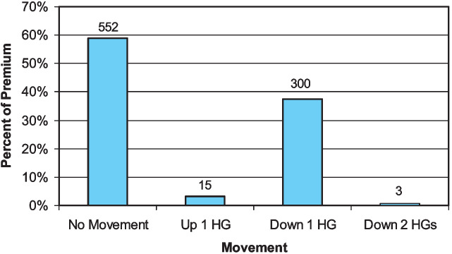
Figure 14 shows that most of the classes and premium remained in the same hazard group when assigned to the new four Hazard Groups. Among those classes that did move, the great majority (300 classes and 37 percent of the premium) moved down one hazard group. Most of this movement was from Hazard Group II to 1. The movements of classes and premium are detailed in Table 5. The table can be read vertically. For instance, among the 428 classes in Hazard Group II, 255 were mapped into Hazard Group 1, 164 into Hazard Group 2, nine into Hazard Group 3, and none into Hazard Group 4. The 255 classes that moved from Hazard Group II into Hazard Group 1 comprised 25.4% of the total premium. A significant number of classes and amount of premium moved from Hazard Group III to 2. Three classes moved from III to 1. Just 15 classes moved up by one hazard group, making up three percent of the premium. Hazard Group 1 is so large primarily because of classes that entered it from Hazard Group II. Hazard Group 2 is quite different than Hazard Group II because many of the classes in 2 originated in III and many of the classes that were in II have moved into 1.

The new seven hazard group assignment has a fairly homogenous distribution of classes and premium, as shown in Figure 15. This distribution is a marked improvement over the prior mapping. In terms of premium, Hazard Group A is 11 times larger than Hazard Group I was. Hazard Group G is twice as large as Hazard Group IV was.

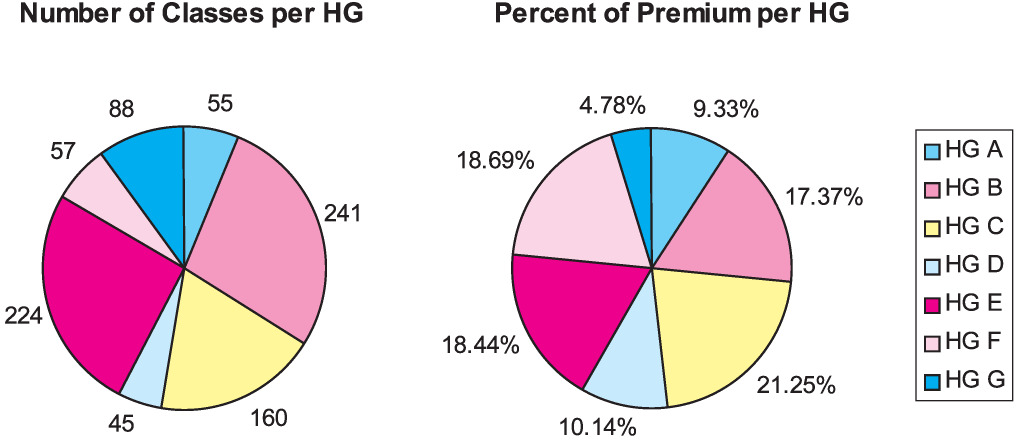
Table 6 shows the distribution of classes to hazard groups based on their level of credibility. Overall there were 162 classes with at least 75 percent credibility and 708 classes with lower credibility. Generally, within each hazard group most of the premium is due to highly credible classes but most of the classes have lower credibility. Hazard Groups D and G are exceptions. Hazard Group D has nearly equal numbers of high and low-credibility classes. In Hazard Group G, high and low-credibility classes have similar premium percentages.

Although Hazard Groups B and E have far more classes than the other hazard groups, they do not have far more premium. The reason that they have the most classes with credibility less than 75 percent is that the complement of credibility is the prior hazard group excess ratio. For instance, the excess ratio of Hazard Group III at $100,000 was 0.451 which is close to the excess ratio of Hazard Group E. Given a small class in Hazard Group III, the credibility-weighted excess ratio was likely to be close to the excess ratio of Hazard Group E.

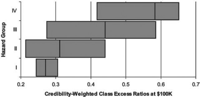
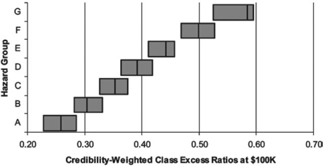
4.2. Range of excess ratios

In Figure 16 each horizontal bar represents the range of credibility-weighted excess ratios within a particular hazard group. The vertical line within each bar represents the overall excess ratio for the hazard group. Among the classes in Hazard Group I, the excess ratios at $100,000 ranged from 0.254 to 0.315. In Hazard Group II, the excess ratios at $100,000 ranged from 0.223 to 0.451. Thus the range of Hazard Group I excess ratios was contained within that of Hazard Group II, indicating that Hazard Groups I and II were not as well separated as might be desired. The same behavior was observed at $1,000,000 as well.

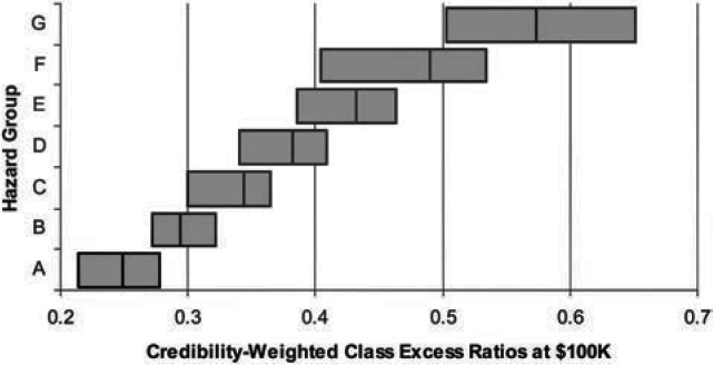
As shown in Figure 17, k-means clustering resulted in well separated hazard groups. Because five dimensions were used, we could not avoid overlap in each dimension, but the excess ratio distribution is a noticeable improvement over the prior mapping. The new mapping also shows a well-separated excess ratio distribution at $1,000,000 as shown in the Figure 18.

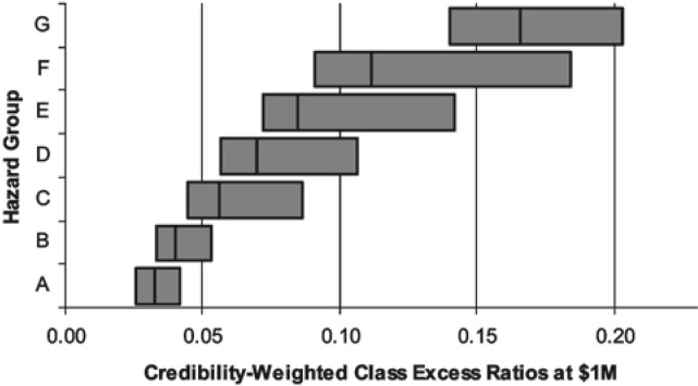
Most of the exposure is concentrated in the largest classes, and so the hazard group excess ratios are highly sensitive to the placement of large classes. In Figures 16–18, the range of excess ratios for each hazard group is calculated using all of the classes in that hazard group.

Figures 19 and 20 show that if ranges are computed using only those classes with at least 75 percent credibility, then the separation of hazard groups by excess ratios is quite strong at both $100,000 and $1,000,000.

5. Underwriting review

After completing the cluster analysis, we conducted a survey of underwriters to solicit their comments on the proposed new mapping. The survey was sent to all members of NCCI’s Underwriting Advisory List (UAL), and included the draft mapping that resulted from the analytic determination of the hazard groups. The survey asked the underwriters to judge the hazardousness of each class based on the likelihood that a given claim would be a serious claim. We also pointed out that if the mix of operations in two classes was very similar then the two classes should probably be in the same hazard group.

Members of the UAL recommended changes in the hazard group assignment for a third of the classes. We also received feedback from two underwriters on staff at NCCI. After the survey comments were compiled, a team consisting of NCCI actuaries and underwriters reviewed the comments from UAL members and decided on the final assignment for each class. When deciding whether to reassign a class, we considered whether the feedback on that class was consistent. We considered the credibility of each class and placed more weight on the cluster analysis results for those classes with a large volume of loss experience. For each class we compared the excess ratios to the overall hazard group excess ratios and identified the nearest two hazard groups.

Class 0030 illustrates the process used at NCCI to decide on the hazard group for each class. This class is for employees in the sugar cane plantation industry and is only applicable in a small number of states. This class

• had 12% credibility,

• was in Hazard Group III under the prior mapping, and

• was assigned to Hazard Group E under the cluster analysis.

An underwriter pointed out that Class 0030 has operations similar to Class 2021, which is for employees who work at sugar cane refining. Insureds in either class can have both farming and refining operations, their class being determined by which operation has the greater payroll. Also, both farming and refining involve use of heavy machinery. Class 2021

• applies nationally,

• had 31% credibility,

• was in Hazard Group II under the prior mapping,

• was assigned to Hazard Group C under the cluster analysis, and

• prior to credibility weighting had excess ratios close to the overall excess ratios for Hazard Group D.

Credibility weighting had reduced Class 2021’s excess ratios so that they were between the overall excess ratios of Hazard Groups C and D, because the prior assignment of Class 2021 had been to Hazard Group II.

We concluded that Hazard Group D was the best choice for 2021 based on its excess ratios prior to credibility weighting and its mix of operations. We determined that 0030 should be assigned to the same hazard group as 2021, so we also assigned Class 0030 to Hazard Group D.

Underwriters made several other types of comments besides those comparing one class to another. For instance, they commented on the degree to which employees in a given class are prone to risk from automobile accidents. They commented on the extent to which heavy machinery is used in various occupations and how much exposure there is to dangerous substances.

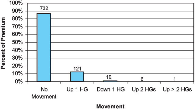
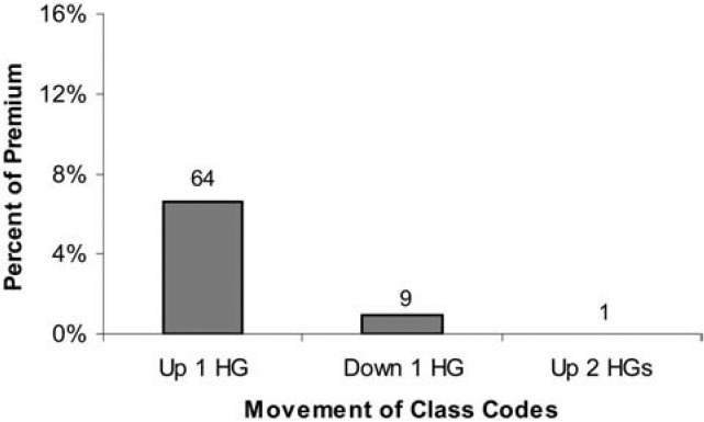
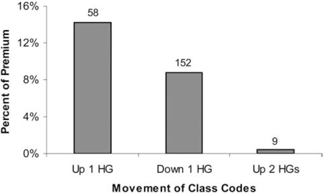
Figure 21 displays the movements of premium and classes during the underwriting review under the collapsed new mapping. It shows that the overall effect of the underwriting review was to move a significant number of classes up to a higher hazard group. The majority of the classes that moved up one hazard group, 78 of them, moved from Hazard Group1 to 2, while 20 classes moved from Hazard Group 2 to 3, and 23 classes moved from Hazard Group 3 to 4.

6. Conclusion

Our approach to remapping the hazard groups was founded on three key ideas.

1. Computing excess ratios by class

   The data is too sparse to directly estimate excess ratios by both class and state. But countrywide excess ratios can be computed by class in the same way that hazard group excess ratios are computed. This does not require separate loss distributions for each class. The existing loss distributions by injury type can be used along with the usual scale assumption. Thus all that is needed is average costs per case by injury type and injury type weights for each class.

2. Sorting classes based on excess ratios

   Rather than using indirect variables to capture the amorphous concept of “excess loss potential,” we used excess ratios directly because hazard groups are indeed used to separate classes based on excess ratios. Because a loss distribution is in fact characterized by its excess loss function, this approach involves no loss of information. By sorting classes based on excess ratios we achieve the goal of sorting classes based on their loss distributions as well.

3. Cluster analysis

   Problems involving sorting objects into groups are not unique to actuarial science. We were thus able to make use of a large statistical literature on cluster analysis. This provided an objective criterion for determining the hazard groups as well as the optimal number of hazard groups. Our approach to determining the seven hazard groups was non-hierarchical because we wanted the best seven group partition and because hypothetical partitions into six hazard groups are not relevant in this context.

As a result of our analysis the number of NCCI hazard groups was increased from four to seven. The distribution of both premium and classes is much more even across the new hazard groups. The highest hazard group is still relatively small. The new seven hazard groups collapse naturally and hierarchically into four hazard groups. Comparing the new four hazard groups with the old, over two-thirds of the classes, with nearly 60% of the premium, did not move at all. This stability was largely a result of the fact that we used the old hazard group as a complement of credibility and there were a large number of classes with very little premium. Of the classes that did move, the overwhelming majority moved down one hazard group.

The new mapping was filed in mid-2006 to be effective with the first rate or loss cost filing in each state on or after January 1, 2007. The filing (Item Filing B-1403) was approved prior to the end of 2006 in all states in which NCCI files rates or loss costs.

---

Acknowledgments

Many staff at NCCI contributed to this paper, including Greg Engl, Ron Wilkins, and Dan Corro. We also thank the NCCI Retrospective Rating Working Group and the NCCI Underwriting Advisory List for their input.

---

1. In published tables, what we denote here as ELFs are often called Excess Loss Pure Premium Factors, or ELPPFs. And in published tables, ratios of excess loss to premium are often called Excess Loss Factors, or ELFs. Some published tables give ratios of excess loss plus allocated loss adjustment expense to either premium or loss plus allocated loss adjustment expense. We are concerned only with ratios of excess losses to total losses.

2. A serious claim is one for which at least one of the following benefits for lost wages is paid or is expected to be paid:
   
   a. Fatal (death)
   
   b. Permanent Total (injured worker not expected to ever be able to work)
   
   c. Permanent Partial (able to work after recovery period, but with a permanent injury, such as loss of a limb) and benefits for lost wages exceed certain thresholds that vary by state and year.

3. Severity is the average claim cost. Indemnity is benefits for lost wages. Medical is benefits for medical costs.

4. Pure premium is the ratio of expected losses to payroll in $100s.

5. See Johnson and Wichern (2002) for a discussion of principal components.

6. We used SAS software, Version 8.2 of the SAS System for a SunOS 5.8 platform.