Robustifying Reserving

All models are wrong but some are useful.

—Christian Dior (or maybe George E. P. Box)

1. Introduction

The idea of this paper is simple. For models using a loss development triangle, the robustness of the model can be evaluated by comparing the derivative of the loss reserve with respect to each data point. All else being equal, models that are highly sensitive to a few particular observations are less preferred than ones that are not. This is supported by the fact that individual cells can be highly volatile. This general approach, based on Tampubolon (2008), is along the lines of robust statistics, so some background into robust statistics will be the starting point. Published models on three data sets will be tested by this methodology. For two of them, unsuspected problems with the previously best-fitting models are found, leading to improved models.

The sensitivity of the reserve estimate to individual points is related to the power of those points to draw the fitted model towards them. This can be measured by what Ye (1998) calls generalized degrees of freedom (GDF). For a model and fitting procedure, the GDF at each point is defined as the derivative of the fitted point with respect to the observed point. If any change in a sample point is matched by the same change in the fitted, the model and fitting procedure are giving that point full control over its fit, so a full degree of freedom is used. GDF does not fully explain the sensitivity of the reserve to a point, as the position of the point in the triangle also gives it more or less power to change the reserve estimate, but it adds some insight into that sensitivity.

Section 2 provides some background of robust analysis, and Section 3 shows some previous applications to actuarial problems. These help to place the current proposal into perspective in that literature. Sections 4, 5, and 6 apply this approach to some published loss development models. Section 7 concludes.

2. Robust methods in general

Classical statistics takes a model structure and tries to optimize the fit of data to the model under the assumption that the data is in fact generated by the process postulated in the model. But in many applied situations, the model is a convenient simplification of a more complex process. In this case, the optimality of estimation methods such as maximum likelihood estimation (MLE) may no longer hold. In fact, a few observations that do not arise from the model assumptions can sometimes significantly distort the estimated parameters when standard techniques are used. For instance, Tukey (1960) gives examples where even small deviations from the assumed model can greatly reduce the optimality properties. Robust statistics looks for estimation methods that in one way or another can insulate the estimates from such distortions.

Perhaps the simplest such procedure is to identify and exclude outliers. Sometimes outliers clearly arise from some other process than the model being estimated, and it may even be clear when current conditions are likely to generate such outliers, so that the model can then be adjusted. If the parameter estimates are strongly influenced by such outliers, and the majority of the observations are not consistent with those estimates, it is reasonable to exclude the outliers and just be cautious about when to use the model.

An example is provided by models of the U.S. one-month treasury bill rates at monthly intervals. Typical models postulate that the volatility of the rate is higher when the rate itself is higher. Often the volatility is proposed to be proportional to the pth power of the rate. The question is—what is p? One model, the CIR or Cox, Ingersoll, Ross model, assumes a p value of 0.5. Other models postulate p as 1 or even 1.5, and others try to estimate p as a parameter. An analysis by Dell’Aquila, Ronchetti, and Troiani (2003) found that when using traditional methods, the estimate of p is very sensitive to a few observations in the 1979–82 period, when the U.S. Federal Reserve bank was experimenting with monetary policy. Including that period in the data, models with p = 1.5 cannot be rejected, but excluding that period finds that p = 0.5 works just fine. That period also experienced very high values of the interest rate itself, so their analysis suggests that using p = 0.5 would make sense unless the interest rate is unusually high.

A key tool in robust statistics is the identification of influential observations, using the influence function defined by Hampel (1968). This procedure looks at statistics calculated from a sample, such as estimated parameters, as functionals of the random variables that are sampled. The influence function for the statistic at any observation is a functional derivative of the statistic with respect to the observed point. In practice, analysts often use what is called the empirical influence. For instance, Bilodeau (2001) suggests calculating the empirical influence at each sample point as the sample size times the decrease (which may be negative) in the statistic from excluding the point from the sample. That is, the influence is n times [statistic with full sample minus statistic excluding the point]. If the statistic is particularly sensitive to a single or a few observations, its accuracy is called into question. The gross error sensitivity (GES) is defined as the maximum absolute value of the influence function across the sample.

The effect on the statistic of small changes in the influential observations is also a part of robust analysis, as these effects should not be too large either. If each observation has substantial randomness, the random component of influential observations has a disproportionate impact on the statistic. The approach used below in the loss reserving case is to identify observations for which small changes have large impacts on the reserve estimate.

Exclusion is not the only option for dealing with outliers. Estimation procedures that use but limit the influence of the outliers are also an important element of robust statistics. Also, finding alternative models which are not dominated by a few influential points and estimating them by traditional means can be an outcome of a robust analysis. In the interest rate case, a model with one p parameter for October 1979 through September 1982 and another elsewhere does this. Finding alternative models with less influence from a few points is what we will be attempting in the reserve analysis.

3. Robust methods in insurance

Several papers on applying robust analysis to fitting loss severity distributions have appeared in recent years. For instance, Brazauskas and Serfling (2000a) focus on estimation of the simple Pareto tail parameter \(\alpha\) assuming that the scale parameter b is known. In this notation the survival function is \(S(x)=(b / x)^\alpha\). They compare several estimators of \(\alpha\), such as MLE, matching moments or percentiles, etc. One of their tests is the asymptotic relative efficiency (ARE) of the estimate compared to MLE, which is the factor which when applied to the sample size would give the sample size needed for MLE to give the same asymptotic estimation error. Due to the asymptotic efficiency of MLE, these factors are never greater than unity, assuming the sample is really from that Pareto distribution.

The problem is that the sample might not be from a simple Pareto distribution. Even then, however, you would not want to identify and eliminate outliers. Whatever process is generating the losses would be expected to continue, so no losses can be ignored.^[1] The usual approach to this problem is to find alternative estimators that have low values of the GES and high values of ARE. Brazauskas and Serfling (2000a) suggest estimators they call generalized medians (GM). The kth generalized median is the median of all MLE estimators of subsets of size k of the original data. That can be fairly calculation-intensive, however, even with small k of 3, 4, or 5.

Finkelstein, Tucker, and Veeh (2006) define an estimator they call the probability integral transform statistic (PITS) which is quite a bit easier to calculate but not quite as robust as the GM. It has a tuning parameter \(t\) in \((0,1)\) to control the trade-off between efficiency and robustness. Since \((b / x)^\alpha\) is a probability and so a number between zero and one, it should be distributed uniformly \([0,1]\). Thus \((b / x)^{t \alpha}\) should be distributed like a uniformly raised to the \(t\) power. The average of these over a sample is known to have expected value \(1 /(t+1)\), so the PITS estimator is the value of \(\beta\) for which the average of \((b / x)^{t \beta}\) over the sample is \(1 /(t+1)\). This is a singlevariable root finding exercise. Finklestein, Tucker, and Veeh give values of the ARE and GES for the GM and PITS estimators, shown in Table 1. A simulation suggests that the GES for MLE for \(\alpha=1\) is about 3.9, and since its ARE is 1.0 by definition, PITS at 0.94 ARE is not worthwhile in this context. In general the generalized median estimators are more robust by this measure.

Other robust severity studies include Brazauskas and Serfling (2000b), who use GM estimation for both parameters of the simple Pareto; Gather and Schultze (1999), who show that the best GES for the exponential is the median scaled to be unbiased (but this has low ARE); and Serfling (2002), who applies GM to the lognormal distribution.

4. Robust approach to loss development

Omitting points from loss development triangles can sometimes lead to strange results, and not every development model can be automatically extended to deal with this, so instead of calculating the influence function for development models, we look at the sensitivity of the reserve estimate to changes in the cells of the development triangle, as in Tampubolon (2008). In particular, we define the impact of a cell on the reserve estimate under a particular development methodology as the derivative of the estimate with respect to the value in the cell. We do this for the incremental triangle, so a small change in a cell affects all subsequent cumulative values for the accident year. This seems to make more sense than looking at the derivative with respect to cumulative cells, whose changes would not continue into the rest of the triangle.

If you think of a number in the triangle as its mean plus a random innovation, the derivative with respect to the random innovation would be the same as that with respect to the total, so a high impact of a cell would imply a high impact of its random component as well. Thus models with some cells having high impacts would be less desirable. One measure of this is the maximum impact of any cell, which would be analogous to the GES, but we will also look at the number of cells with impacts above various thresholds in absolute value.

This is just a toe in the water of robust analysis of loss development. We are not proposing any robust estimators, and will stick with MLE or possibly quasi-likelihood estimation. Rather we are looking at the impact function as a model selection and refinement tool. It can be used to compare competing models of the same development triangle, and it can identify problems with models that can guide a search for more robust alternatives. This is similar to finding models that work for the entire history of interest rate changes and are not too sensitive to any particular points.

To help interpret the impact function, we will also look at the generalized degrees of freedom (GDF) at each point. This is defined as the derivative of the fitted value with respect to the observed value. If this is near 1, the point’s initial degree of freedom has essentially been used up by the model. The GDF is a measure of how much a point is able to pull the fitted value towards itself. Part of the impact of a point is this power to influence the model, but its position in the triangle also can influence the estimated reserve. Just like with the impact function, high values of the GDF would be a detriment.

For the chain-ladder (CL) model, some observations can be made in general. All three corners of the triangle have high impact. The lower left corner is the initial value of the latest accident year, and the full cumulative development applies to it. Since this point does not affect any other calculations, its impact is the development factor, which can sometimes be substantial. The upper right corner usually produces a development factor which, though small, applies to all subsequent accident years, so its impact can also be substantial. When there is only one year at ultimate, this impact is the ratio of the sum of all accident years not yet at ultimate, developed to the penultimate lag, to the penultimate cumulative value for the oldest accident year. The upper left corner is a bit strange in that its impact is usually negative. Increasing it will increase the cumulative loss at every lag, without affecting future incrementals, so every incremental-to-previous-cumulative ratio will be reduced. The points near the upper right corner also tend to have high impact, and those near the upper left tend to have negative impact, but the lower left point often stands alone in its high impact.

The GDFs for CL are readily calculated when factors are sums of incrementals over sums of previous cumulatives. The fitted value at a cell is the factor applied to the previous cumulative, so its derivative is the product of its previous cumulative and the derivative of the factor with respect to the cell value. But that derivative is just the reciprocal of the sum of the previous cumulatives, so the GDF for the cell is the quotient of its previous cumulative and the sum. Thus these GDFs sum down a column to unity, so each development factor uses up a total GDF of 1.0. Essentially each factor uses 1 degree of freedom, agreeing with standard analysis. The average GDF in a column is thus the reciprocal of the number of observations in that column. Thus the upper right cell uses 1 GDF, the previous column’s cells use ½ each on average, etc. Thus the upper right cells have high GDFs and high impact.

We will use ODP, for overdispersed Poisson, to refer to the cross-classified development model in which each cell mean is modeled as a product of a row parameter and a column parameter, the variance of the cell is proportional to its mean, and the parameters are estimated by the quasi-likelihood method. It is well known that this model gives the same reserve estimate as CL. Thus if you change a cell slightly, the changed triangle will give the same reserve under ODP and CL. Thus the impacts of each cell under ODP will be the same as those of CL. The GDFs will not be the same, however, as the fitted values are not the same for the two models. The CL fitted value is the product of the factor and the previous cumulative, whereas the ODP cumulative fitted values are backed down from the latest diagonal by the development factors, and then differenced to get the incremental fitted. It is possible to write down the resulting GDFs explicitly, but it is probably easier to calculate them numerically.

It may be fairly easy to find models that reduce the impact of the upper right cells. Usually the development factors at those points are not statistically significant. Often the development is small and random, and is not correlated with the previous cumulative values. In such cases, it may be reasonable to model a number of such cells as a simple additive constant. Since several cells go into the estimation of this constant, the impact of some of them is reduced. Alternatively, the factors in that region may follow some trends, linear or not, that can be used to express them with a small number of parameters. Again, this would limit the impact of some of the cells.

The lower left point is more difficult to deal with in a CL-like model. One alternative is a Cape-Cod type model, where every accident year has the same mean level. This can arise, for instance, if there is no growth in the business, but also can be seen when the development triangle consists of on-level loss ratios, which have been adjusted to eliminate known differences among the accident years. In this type of model, all the cells go into estimating the level of the last accident year, so the lower left cell has much less impact. This reduction in the impact of the random component of this cell is a reason for using on-level triangles.

The next three sections illustrate these concepts using development triangles from the actuarial literature. The impacts and GDFs are calculated for various models fit to these triangles. The impacts are calculated by numerical derivatives, as are the GDFs except for those for the CL, which have been derived above.

5. A development-factor example

5.1. Chain ladder

Table 2 is a development triangle used in Venter (2007b). Note that the first two accident years are developed all the way to the end of the triangle, at lag 11. Table 3 shows the impact of each cell on the reserve estimate using the usual sum/sum development factors. In the CL model an explicit formula can be derived for these impacts, but it is easier to do the derivatives numerically, simply by adding a small value to each cell separately and recalculating the estimated reserve to get the change in reserve for the derivative.

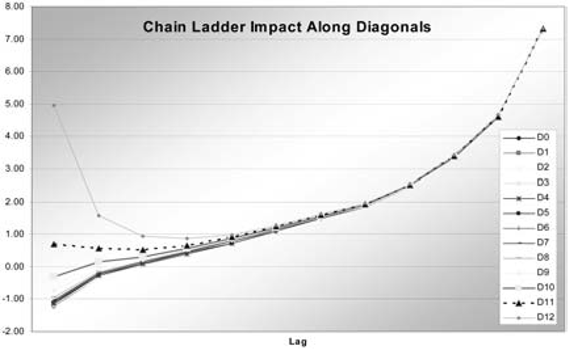
As discussed, the impacts are highest in the upper right and lower left corners, and the upper left has negative impact. The impacts increase moving to the right and down. The last four columns and the lower left point have impacts greater than 2, and six points have impacts greater than 4. Table 4 shows the GDFs for the chain ladder using the formula previous cumulative/sum previous cumulatives derived in Section 4. L0’s GDFs are shown as identically 1.0. Like the impact function, except for lag 0, these increase from one column to the next. Within each column the sizes depend on the volume of the year. Figure 1 graphs the impacts by lag along the diagonals of the triangle. After the first four lags, the impacts are almost constant across diagonals.

Figure 1.Impact of chain ladder by diagonal

5.2. Regression model

Venter (2007b) fit a regression model to this triangle, keeping the first 5 development factors but including an additive constant. The constant also represents development beyond lag 5. By stretching out the incremental cells to be fitted into a single column Y, this was put into the form of a linear model Y = Xβ + ε, which assumes a normal distribution of residuals with equal variance (homoscedasticity) across cells. X has the previous cumulative for the corresponding incrementals, with zeros to pad out the columns, a column of 1s for the constant. There were also diagonal (calendar year) effects in the triangle. Two diagonal dummy variables were included in X, one with 1s for observations on the 4th diagonal and 0 elsewhere, and one equal to 1 on the 5th, 8th, and 10th diagonals, −1 on the 11th diagonal, and 0 elsewhere. The diagonals are numbered starting at 0, so the 4th is the one beginning with 8,529 and the 10th starts with 19,373. The variance calculation used a heteroscedasticity correction. This model with 8 parameters fit the data better than the development factor model with 11 parameters. Here we are only addressing the robustness properties, however.

Table 5 gives the impact function for this model. It is clear that the large impacts on the right side have been eliminated by using the constant instead of factors to represent late development. The effects of the diagonal dummies can also be seen, especially in the right of the triangle. Now only one point has impact greater than 2, and one greater than 4.

Table 6 shows the GDFs for the regression model. For regression models the GDFs for the observations in the Y vector are known to be calculable as the diagonal of the “hat” matrix, where hat = X(X′X)⁻¹X′, e.g., see Ye [2]. However in development triangles, changing an incremental value also changes subsequent cumulatives, so the X matrix is a function of lags of Y. This requires the derivatives to be done numerically. The total of these, excluding lag 0, is 8.02, which is a bit above the usual number of parameters, due to the exceptions to normal linear models. Compared to the CL, the GDFs are lower for lag 6 onward, but are somewhat higher along the modeled diagonals. They are especially high for diagonal 4, which is short and gets its own parameter.

Figure 2 graphs the impacts. Note that due to the diagonal effects, diagonal 11 has higher impact than diagonal 12 after the first two lags.

Figure 2.Impact of regression model by diagonal

5.3. Square root regression model

As a correction for heteroscedasticity, regression courses sometimes advise dividing both Y and X by the square root of Y, row by row. This makes the model Y^1/2 = (X/Y^1/2)β + ε, where the ε are IID mean zero normals. Then Y = Xβ + Y^1/2ε, so now the variance of the residuals is proportional to Y. This sounds like a fine idea, but it is a catastrophe from a robust viewpoint. Table 7 shows the impact function. There are 12 points with impact over 2, seven with impact over 4, five with impact over 10, and three with impact over 25.

Part of the problem is that the equation Y = Xβ + Y^1/2ε is not what you would really want. The residual variance should be proportional to the mean, not the observations. This setup gives the small observations small variance, and so the ability to pull the model towards them. But the observations might be small because of a negative residual, with a higher expected value. So this formulation gives the small values too much influence.

Table 8 shows the related GDFs. It is unusual here that some points have GDFs greater than 1. A small change in the original value can make a greater change in the fitted value, but due to the non-linearity the fitted value is still not exactly equal to the data point. The sum of the GDFs is 13.0, which is sometimes interpreted as the implicit number of parameters.

5.4. Gamma-p residuals

Venter (2007a) fits the same regression model using the maximum likelihood with gamma-p residuals. The gamma-p is a gamma distribution, but each cell is modeled to have the variance proportional to the same power p of the mean. This models the cells with smaller means as having smaller variances. However, the effect is not as extreme as in the square root regression, where the variance is proportional to the observation, not its expected value.

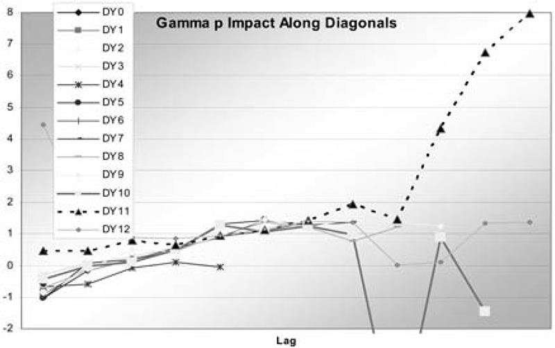
In this case, p was found to be 0.71. The impacts are shown in Table 9 and graphed in Figure 3. It is clear that these are not nearly as dramatic as the square root regression, but worse than the regular regression, and perhaps comparable to the chain ladder. Diagonals 10 and 11 can be seen to have a few significant impacts. These are at points with small observations that are also on modeled diagonals. Even with the variance proportional to a power of the expected value, these points still have a strong pull. The GDFs are in Table 10.

Figure 3.Impact of gamma-p residual model

Again this is less dramatic than for the square root regression, but the small points on the modeled diagonals still have high GDFs. The total of these is 11.3, which is still fairly high. This is somewhat troublesome, as the gamma-p model fit the residuals quite a bit better than did the standard regression. The fact that the problems center on small observations on the modeled diagonals suggests that additive diagonal effects may not be appropriate for this data. They do fit into the mold of a generalized linear model, but that is not too important when fitting by MLE anyway. As an alternative, the same model but with the diagonal effects as multiplicative factors was fit. The multiplicative diagonal model can be written:

\[ \mathbf{E Y}=\mathbf{X}[, 1: 6] \boldsymbol{\beta}[1: 6] * \boldsymbol{\beta}[7]^{\mathbf{X}[, 7]} * \boldsymbol{\beta}[8]^{\mathbf{X}[, 8]}, \]

which means that the first six columns of X are multiplied by the first six parameters, which includes the constant term, and then the last two diagonal parameters are factors raised to the power of the last two columns of X. These are now the diagonal dummies, which are 0, 1, or −1. Thus the same diagonals are higher and the same lower, but now proportionally instead of by an additive constant. It turns out that this model actually fits better, with a negative loglikelihood of 625, compared to 630 for the generalized linear model. This solves the robustness problems as well. The impacts are in Table 11, the GDFs in Table 12, and the impacts are graphed in Figure 4.

Figure 4.Impact of gamma-p multiplicative model

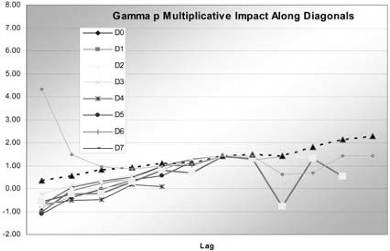
Diagonal 11 still has more impact than the others, but this barely exceeds 2.0 at the maximum. The sum of the GDFs is 8.67. There are eight parameters for the cell means but two more for the gamma-p. It has been a question whether or not to count those two in determining the number of parameter used in the fitting. The answer to that from the GDF analysis is basically to count each of those as 1/3 in this case. Here the robust analysis has uncovered a previously unobserved problem with the generalized linear model, and lead to an improvement.

6. A multiplicative fixed-effects example

A multiplicative fixed-effects model is one where the cell means are products of fixed factors from rows, columns, and perhaps diagonals. The most well known is the ODP model discussed in Section 4, where there is a factor for each row, interpreted as estimated ultimate, a factor for each column, interpreted as fraction of ultimate for that column, and the variance of each cell is a fixed factor times its mean. This model if estimated by MLE gives the same reserve estimates as the chain ladder and so the same impacts for each cell, but the GDFs are different, due to the different fitted values.

The triangle for this example comes from Taylor and Ashe (hereafter TA; 1983) and is shown in Table 13. The CL = ODP impacts are in Table 14 and are graphed in Figure 5.

Figure 5.Impact of CL = ODP on TA

Because the development factors are higher, the impacts are higher than in the previous example. Even though it is a smaller triangle, 14 points have impacts with absolute values greater than 2, four are greater than 4, and two are greater than 12. The CL GDFs are in Table 15. These sum to 9, excluding the first column, and are fairly high on the right where there are few observations per column. The ODP GDFs are in Table 16. These sum to 19, and are fairly high near the upper right and lower left corners.

The GDFs can be used to allocate the total degrees of freedom of the residuals of n − p. The n is allocated equally to each observation, and the p can be set to the GDF of each observation. This would give a residual degree of freedom to each observation which could be used in calculating a standardized residual that takes into account how the degrees of freedom vary among observations.

Venter (2007b) looked at reducing the number of parameters in this model by setting parameters equal if they are not significantly different, and using trends, such as linear trends, between parameters. Also, diagonal effects were introduced. The result was a model where each cell mean is a product of its row, column, and diagonal factors. There are six parameters overall. For the rows there are three parameters, for high, medium, and low accident years. Accident year 0 is low, year 7 is high, year 6 is the average of the medium and high levels, and all other years are medium. There are two column factors: high and low. Lags 1, 2, and 3 are high, lag 4 is an average of high and low, lag 0 and lags 5 to 8 are low, and lag 9 is 1 minus the sum of the other lags. Finally there is one diagonal parameter c. Diagonals 4 and 6 have factors 1 + c, lag 7 has factor 1 − c, and all the other diagonals have factor 1.

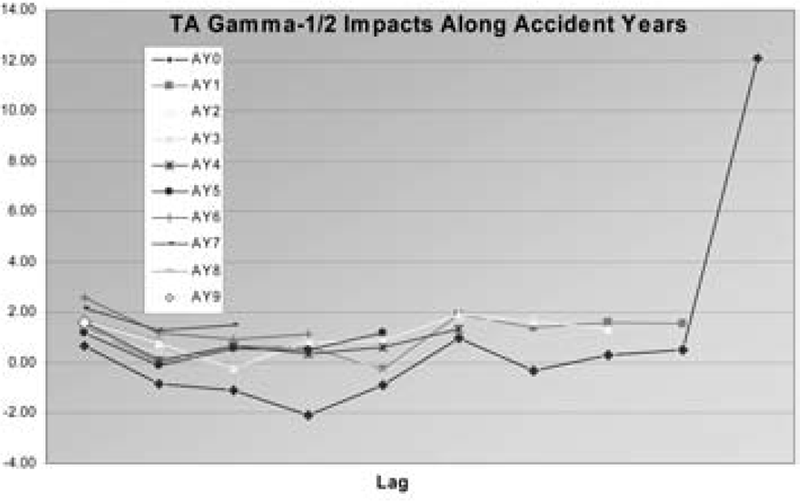
With just six parameters this model actually provides a better fit to the data than the 19 parameter model. The combining of parameters does not degrade the fit much, and adding diagonal effects improves the fit. An improved fit over that in Venter (2007b) was found by using a gamma-p distribution with p = ½ so the variance of each cell is proportional to the square root of its mean. The impacts and GDFs of this model are shown in Tables 17 and 18, and the impacts are graphed in Figure 6, this time along accident years.

Figure 6.Impact of gamma-\(\frac{1}{2}\) on TA

The impacts are now all quite well contained except for one point—the last point in AY0. Possibly because AY0 gets its own parameter, lag 9 influences the level of the other lags’ parameters, and this is a small point with a small variance, this model only slightly reduces the high level of impact that point has in ODP. The same thing can be seen in the GDFs as well, where this point has slightly less than a whole GDF. The points on AY7 and the modeled diagonals also have relatively high GDFs, as do some small cells. The total of the GDFs is 6.14. There are six parameters affecting the means, plus one for the variance of the gamma. That one can affect the fit slightly, so counting it as 1/7th of a parameter seems reasonable.

In an attempt to solve the problem of the upper-right point, an altered model was fit: lag 9 gets half of the paid in the low years. This can be considered a trend to 0 for lag 10. Making the lags sum to 1.0 now eliminates a parameter, so there are five. The negative loglikelihood (NLL) is slightly worse, at 722.40 vs. 722.36, but that is worth saving a parameter. The robustness is now much better, with only two impacts greater than 2.0, the largest being 2.35.

7. Paid and incurred example

Venter (2008), following Quarg and Mack (2004), builds a model for simultaneously estimating paid and incurred development, where each influences the other. The paid losses are part of the incurred losses, so the separate effects are from the paid and unpaid triangles, shown in Tables 19 and 20.

First, the impacts on the reserve (7059.47) from the average of the paid and incurred chain ladder reserves are calculated, where the paids at the last lag are increased by the incurred-to-paid ratio at that lag. Tables 21 and 22 show the impacts of the paid and unpaid triangles, and Tables 23 and 24 show the GDFs.

The impacts of the lower left are not great, mostly because the development factors are fairly low in this example. The impacts on the upper right of both paid and unpaid losses are quite high, however. The unpaid losses other than the last diagonal have a negative impact, because they lower subsequent incurred development factors, but do not have factors applied to them. The GDFs are similar to CL in general.

The model in Venter (2008) used generalized regression for both the paid and unpaid triangles, where regressors could be from either the paid and unpaid triangles or from the cumulative paid and incurred triangles. Except for the first couple of columns, the previous unpaid losses provided reasonable explanations of both the current paid increment and the current remaining unpaid. The paid and unpaid at lags 3 and on were just multiples of the previous unpaid, with a single factor for each. That is, expected paids were 33.1%, and unpaids 72.3%, of the previous unpaid. Since these sum to more than 1, there is a slight upward drift in the incurred. The lag 2 expected paid was 68.5% of the lag 1 unpaid. The best fit to the lag 2 expected unpaid was 9.1% of the lag 1 cumulative paid. For lag 1 paid, 78.1% of the lag 0 incurred was a reasonable fit. Lag 1 unpaid was more complicated, with the best fit being a regression, with constant, on lag 0 and lag 1 paids. There were also diagonal effects in both models. The residuals were best fit with a Weibull distribution. Tables 25–28 show the fits.

The two highest impacts for the average of paid and incurred are 14 and 15. For the Weibull they are 7.7 and 5.5. The average has two other points with impacts greater than 5, whereas the Weibull has none. Below 5 the impacts are roughly comparable. Since the Weibull has variance proportional to the mean squared, small observations have lower variance, and so a stronger pull on the model and higher impacts. In total, excluding the first column, the GDFs sum to 9.9, but including the diagonals (see Venter 2008 for details) there are 12 parameters plus two Weibull shape parameters. The form of the model apparently does not allow the parameters to be fully expressed. The Weibull model still has more high impacts than would be desirable, but it is a clear improvement over the average of the paid and incurred. The reserve is quite a bit lower for the better fitting Weibull model as well: 6255 vs. 7059.

8. Conclusion

Robust analysis has been introduced as an additional testing method for loss development models. It is able to identify points that have a large influence on the reserve, and so whose random components would also have a large influence. Through three examples, customized models were found to be more robust than standard models like CL and ODP, and in two of the examples, even better models were found as a response to the robust analysis.