Economic Impact of Capital Level in an Insurance Company

1. Introduction

An insurer’s policyholder surplus changes primarily through retained earnings. Insurance companies can also manipulate surplus by issuing new shares, paying out dividends, or buying back shares. Changes in surplus level have complex effects on shareholder return. Our goal is to provide a thorough analysis of these effects. We apply various financial economic theories to insurance, including the Modigliani-Miller irrelevance theorem, the theory of frictional costs, and the theory of risk capital developed in Merton and Perold (1993). Economic capital, defined by market values of assets and liabilities, will be the basis of our analysis instead of accounting surplus. The change in shareholder wealth is more easily explained in terms of economic capital than accounting surplus.

Capital level has significant impact on premium adequacy. Policyholders are concerned about an insurer’s ability to pay claims. If the insurer holds an insufficient amount of capital, it is likely to default on claims, so the market value of the actual claim payment is less than the claim’s full value. Consequently, policyholders require premium credits. The question is whether the premium credit exactly offsets the reduction in covered loss (so the expected profit remains unchanged) or the premium falls more than the covered loss (so the expected profit declines). We will answer this question using the solvency guarantee. An insurance company may purchase a solvency guarantee to eliminate its default risk. Merton and Perold (1993) find that issuing policies with default risk is economically equivalent to buying a solvency guarantee from policyholders. This observation is used to prove that the premium credit is greater than the market value of uncovered liability. Thus, an inadequately capitalized company is less profitable than a default-free competitor.

The presence of frictional costs is another reason why shareholder return is sensitive to the capital level. The effect of frictional costs is better understood by first examining an ideal case—when these costs do not exist. We prove that, in a default-free firm with no frictional costs, shareholders are indifferent to the capital level. This is an insurance version of the Modigliani-Miller irrelevance theorem. Holding less capital, the firm produces higher return on shareholder equity (ROE). But this benefit is exactly offset by higher volatility risk. The indifference statement, however, breaks down when frictional costs do exist. Frictional costs reduce shareholder return, and the capital level affects the magnitude of frictional costs tremendously.

Frictional costs in an insurance firm can be roughly divided into the frictional cost of capital and the cost of financial distress. Corporate taxes and agency costs are examples of the first class. The second class includes direct and indirect bankruptcy costs. A change in capital level increases one class of costs and reduces the other. Perold (2005) captures these costs in a simple model for financial firms. He finds an optimal capital level that minimizes total frictional costs. We apply his line of arguments to insurance firms.^[1]

In Section 2, we first examine and define some basic concepts, then employ the solvency guarantee to study the premium credit. In Section 3, we prove that changes in capital level do not affect shareholder wealth in a default-free firm with zero frictional costs. Frictional costs are defined and discussed in Section 4. Under acceptable assumptions, a unique optimal level of capital exists that minimizes total frictional costs. We briefly comment on related unresolved issues in Section 5.

2. Impact of capital level on premium

2.1. Fair value of insurance liabilities

Stocks and bonds are traded on open markets; their market values are directly observable. The market values can be expressed as present values of future cash flows, such as dividends and interest. Discount rates used for computing the present values are usually greater than risk-free rates with comparable durations, since investors expect higher rates of return from risky assets. This discounted cash flow (DCF) approach is also used by actuaries to calculate present values of insurance liabilities. Most liabilities are not traded on active markets. Companies make their own judgment in choosing discount rates. Therefore, for a given liability whose settlement value and timing are random, there is considerable disagreement on its present value. However, an objective valuation approach appears to be necessary. In a reinsurance transaction, for example, the cedant, the reinsurers, and the regulators all need to agree on the value of the ceded liabilities. In a merger or acquisition, company shareholders, lenders, and regulators also demand a fair and objective valuation of the liabilities. In recent years, regulators and insurance practitioners have debated extensively on the basic principles of fair valuation. The fair value of a liability is generally perceived to be independent of the company that holds it, and it reflects the market risk, not the unique risks pertaining to a company.^[2] In this paper, we simply assume the fair values exist and satisfy some intuitive conditions.^[3] This will provide us a convenient platform for discussing the impact of capital level.

Consider the following one-period model. Insurance policies are issued at time 0 and claims settled at time 1. A policy liability is a random variable L, whose time-0 market value is denoted by l. An asset is a random variable A, with market value a at time 0. We introduce a market value function, V(·), for both assets and liabilities. Thus V(A) = a and V(L) = l. Let E[A] and E[L] be the expected values, and r the risk-free rate. If A is a risky asset, V(A) is generally less than E[A]/(1 + r), where the difference represents a risk margin. Similarly, for a risky liability L, V(L) is greater than or equal to E[L]/(1 + r), depending on whether or not L contains systematic risks. We further assume V(·) is additive,^[4] and is applicable to mixtures of assets and liabilities. Thus V(A − L) = a − l. The following intuitive conditions should also hold:

1. V(·) is positive: if A > 0 then V(A) > 0, and if L > 0 then V(L) > 0.

2. If A or L is nonrandom, then V(A) = A/(1 + r), V(L) = L/(1 + r). In particular, V(0) = 0, where the 0 in the V function stands for a zero asset or a zero liability.

3. V(·) is continuous, which roughly means a small change in A or L results in a small change in V(A) or V(L).

Calculation of present values is not our concern in this paper.^[5]

2.2. The default-adjusted balance sheet

Insurance premium covers claim liabilities, expenses, and frictional costs. The expenses are the normal business costs for marketing, underwriting, claim adjusting, and investment, all of which are roughly independent of the capital level. In this paper we consider the premium as net of expenses. Categories of frictional costs include income taxes, agency costs, and costs of financial distress. In this and the following sections, we assume the frictional costs to be zero. We will devote all of Section 4 to the effect of frictional costs.^[6]

Consider an insurance company that holds an initial shareholder capital c but no debt and writes insurance policies for a total net premium p. The total liability is a random variable L, which will be paid at time 1. l = V(L). The initial asset value of the company is a ≡ p + c. Assume the assets are invested in a portfolio of bonds and stocks, and the random rate of return is R. Then the total asset value at time 1 is A = a(1 + R) = (p + c)(1 + R). k ≡ a − l is called the actuarial surplus. We have the following market value balance sheet:

.

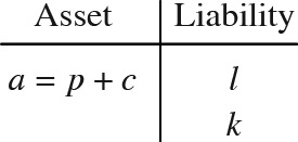
On the statutory or GAAP balance sheets, not all assets and liabilities are booked consistently with the market. For instance, bonds may be carried at amortized cost, and most property/casualty liabilities are not discounted. The market value balance sheet better reflects the shareholder value, so is more relevant in pricing and risk management.

In the above balance sheet, the liability is valued as if it would be fully paid at time 1. In fact, when a company becomes insolvent, policyholders cannot recover their losses in full. So if there is a chance of insolvency, the true value of a liability is less than its market value. Consequently, the true value of the policyholder surplus is greater than the actuarial surplus k. We now restate the balance sheet to show these effects explicitly.

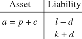
A company becomes insolvent at time 1 if L > A. Upon insolvency the insurer pays out the entire asset A to policyholders and assumes no more liability. The amount of policyholder unrecoverable loss is D ≡ max(L − A, 0). D is often viewed as a put option, called the default put or the insolvency put. It is owned by the shareholders and exercised at default. The price of the default put, d ≡ V(D), is also known in the actuarial literature as the expected value of default, or the expected policyholder deficit. Clearly, the time-1 actual payoff is L − D. So the true value of the liability is V(L − D) = l − d, and the true policyholder surplus is a − (l − d) = k + d. The default-adjusted (market value) balance sheet is as follows:

.

The net asset at time 1, after claims are paid off, is A − L if the company remains solvent, or zero if it defaults. So the net asset can be written as A − L + D. The surplus, k + d, is thus the market value of the net asset. The default-adjusted balance sheet and its equivalents have been discussed in many papers. See Merton and Perold (1993), Myers and Read (2001) and Sherris (2006) for a few examples.

2.3. Solvency guarantee

A company may purchase insurance to cover its default risk. Such an insurance is called a solvency guarantee. When the company defaults, the guarantor takes over the remaining claims. A company may buy a full solvency guarantee to become default-free, or a partial guarantee to reduce its default risk. An actual guarantee does not have to be purchased in an insurance transaction. It may take the form of a parent guarantee or a market guaranty fund. Regardless of the form, the company, or another party on its behalf, pays a price to get the guarantee. A market fund (in the U.S., a state fund) is accumulated by assessing all participating companies. To be fair, the amount of assessment should vary directly with a company’s potential default cost. For example, an AAA-rated company should pay a low assessment, because it has little chance to consume the fund itself. The actual assessment, however, is usually a percentage of net written premium. This funding mechanism is simple to manage, but lacks fairness. If a parent firm serves as a guarantor, a liability item enters its balance sheet which presumably equals the present value of potential payout. This liability is part of the price paid by the parent firm (to itself) on behalf of the subsidiary. The parent firm also incurs accounting and administrative expenses associated with the guarantee, which should be viewed as another part of the price.

Merton and Perold (1993) observe that issuing policies with default risk is equivalent to purchasing a solvency guarantee from policyholders. Thus the insurer needs to pay the policyholders for the guarantee. This payment is actually a premium deduction. In the real world, policyholders always bear some default risk. No company is default-free. Even with the guarantee of a market fund or a parent firm, there is still residual risk to policyholders. Recoveries from a fund may be limited in amount, or they may be delayed and cause financial inconvenience. A parent firm may have its own financial trouble, and thus be unable to fulfill its obligations. Therefore, policyholders always supply part of the guarantee. Under this view of Merton and Perold (1993), every company is covered by a full solvency guarantee, which may be a combination of more than one partial guarantees—for example, a primary one from a guaranty fund and a residual one from policyholders.

Merton and Perold (1993) point out that the prices paid for various forms of full guarantees are approximately the same, since they all cover the same liability at default. But each guarantee has its own expenses and frictional costs, so the prices are not exactly equal.

2.4. Impact of capital level on premium

If insurance markets are competitive, the policy premium should be just high enough to cover claim liabilities, expenses, and frictional costs. This is called the fair or the competitive premium. In equation,

$$\begin{aligned} \text { Premium }= & V(\text { Claim Liability })+\mathrm{PV}(\text { Expense }) \\ & +\mathrm{PV}(\text { Frictional Cost }) \end{aligned} \tag{2.1}$$

where V(·) is the market value function and PV stands for the present value. (Expenses and frictional costs are not traded, so they do not have market values. Their present values may be calculated by an appropriate discounted cash flow approach.) In a default-free insurance company, the liability L will be fully paid at time 1. We continue to assume there is no frictional cost. Use p₀ to denote the competitive premium (net of expenses) charged by a default-free company. Then p₀ = l = V(L). If a company is not default-free, then its claim liability is L − D, which is less than the full liability L. So the corresponding premium, p, must be less than p₀. We discuss the premium deduction in the remainder of the section.

Assume the policyholders have the freedom to choose between two insurance companies. Company #1 is default-free and charges competitive premium $p_0$. Company #2 has a chance of default, but purchases a full solvency guarantee to eliminate the default risk. Since the policyholders see no difference between the two companies, they would pay the same amount of premium, $p_0$, to Company #2. Let $p_g$ be the price Company #2 pays for the solvency guarantee.^[7] Then its net premium is $p \equiv p_0-p_g$. It charges less premium than does Company #1, but covers less liability as well.

The guarantor is liable for the amount $L-A$ when $L-A>0$. This liability exactly equals the policyholders’ unrecoverable loss $D=$ $\max (L-A, 0)$. Its market value is $d=V(D)$. The guarantor’s premium $p_g$ should cover $d$ and the guarantor’s expenses and frictional costs. Thus $p_g>d$, and $p=p_0-p_g<p_0-d=l-d$.

Here are some details on a guarantor’s expenses and frictional costs. If the guarantor is a market fund, it incurs administrative expenses. Since assessments are not always fair, additional political problems and legal costs may exist. A parent firm has accounting and monitoring expenses associated with the guarantee. When a guarantee is bought from the policyholders, which is to say the policies are issued with default risk, the policyholders incur more costs than simply taking back uncovered claims. Unrecoverable claims are correlated with policyholders’ own losses, so may cause additional pain. Also, policyholders may have to pay expenses on arbitrations and lawsuits, and may experience delay in recoveries. Usually a guarantor’s expenses are funded by the insurance company, although a parent firm may absorb them as its own expenses.

If policies are issued from an insurance firm with default risk, then $p_g$ is the premium deduction, relative to the full premium $p_0$ charged by a default-free firm. The inequality $p=p_0-p_g<$ $p_0-d$ means that, when the market value of covered liability is reduced by $d$, the corresponding premium decreases more than $d$. Empirical studies by Sommer (1996) and Phillips, Cummins, and Allen (1998) confirm that premium declines as the probability of default increases. Further, Wakker, Thaler, and Tversky (1997) and Phillips, Cummins, and Allen (1998) observe that premium credits required by policyholders are often many times more than the expected value of default. Some interesting explanations can be found in Wakker, Thaler, and Tversky (1997) and Froot, Venter, and Major (2004). We provided a simple one above using the solvency guarantee.

From Equation (2.1), the fair premium (net of expenses, with zero frictional costs) that should be charged by a not-default-free firm equals $l-d$. However, if a default-free competitor exists, this firm has to lower the premium to $l-p_g$. Thus, financially weak firms cannot make a fair profit. (However, in a hard market all firms may charge higher-than-fair premiums. Thus, even weak firms make a profit, although not as high as a default-free competitor does.) The loss in profit, on the market value basis, is $p_g-$ $d\left(=(l-d)-\left(l-p_g\right)\right)$. This argument can be extended slightly. Suppose two firms, having different chances of default, compete for the same business. They each purchase a solvency guarantee from policyholders. Policyholders of the firm with a greater chance of default are more likely to incur expenses and frictional costs associated with the guarantee (arbitration, lawsuits, and delay in recovery), and require higher premium credit to cover them. Thus, this firm charges less adequate premium, and its profit falls more than the other firm’s.

3. Return on shareholder equity

An insurance firm may reduce its capital level by paying dividends or buying back shares, or it may raise more capital by issuing new shares. At first glance, shareholders should prefer a lower level of capital, since the return on capital increases as the denominator decreases. But this is not true. Under proper assumptions, shareholder wealth does not change with capital level. The Modigliani-Miller (MM) theory solves this problem beautifully.

Modigliani and Miller published a series of papers in the 1950s and 1960s on how financing decisions affect firm value. A recent review of this work is Rubinstein (2003). MM’s Proposition I (MMI) states that the value of a firm is independent of its debt-equity ratio. Other MM propositions deal with the cost of capital, dividend policy, and shareholder value. The original MM applies to product firms. To extend it to the insurance world, we may view the insurance liability as a risky debt, and the liability to surplus ratio as the debt-equity ratio. Some parallel statements can be made intuitively; see Vaughn (1998). However, the insurance problem has its unique features. Firm assets are mostly bonds and stocks, so can be replicated by investors. Change in capital level affects premium adequacy. An insurance firm’s main activity is on the liability side of the balance sheet, unlike that of product firms. Thus, a fresh and rigorous treatment seems warranted.

3.1. Capital irrelevance in default-free firms

Consider an insurance company with equity financing but no debt. It has a preset strategy for investing the premium. Regardless of capital and premium levels, the premium is always invested in a stock and bond portfolio with a fixed fraction in each security. Let R be the rate of return of the portfolio. In this subsection, we assume the company is default-free. Define the insurance profit as Y ≡ p(1 + R) − L. It is the profit generated by policyholder-supplied funds. The market value of insurance profit, y = p − l, is independent of how the premium is invested.^[8]

Suppose two insurance companies have different capital levels but are identical otherwise. Company #1 holds initial capital $c_1$ and insures liability $L_1$, and Company #2 holds capital $c_2$ and liability $L_2 . c_1>c_2$, and $L_1$ and $L_2$ are identically distributed and perfectly correlated random variables. Thus $L_1$ and $L_2$ have the same market value, $l \equiv V\left(L_1\right)=V\left(L_2\right)$.^[9] Assume $c_1$ and $c_2$ are so large that both companies are default-free, and the companies charge the same competitive premium (net of expenses, with zero frictional costs) $p \equiv p_1=p_2$. The premiums are invested in the same stock and bond portfolio with risky return $R$. We first examine the case that the capitals are invested risk-free. The insurance profit of each company is $Y_j=p(1+R)-L_j$, which are also identically distributed and perfectly correlated, with the same market value $y=V\left(Y_1\right)=$ $V\left(Y_2\right)=p-l$.

Suppose an investor holds an amount of cash c₁. He may either invest the entire c₁ in Company #1, or invest an amount c2 in Company #2 and the rest, c₁ − c₂, in the risk-free asset. By the second strategy, at time 1, the investor receives net asset p(1 + R) + c₂(1 + r) − L₂ = Y₂ + c₂(1 + r) from Company #2, and (c₁ − c₂)(1 + r) from the risk-free asset. The total amount is Y₂ + c₁(1 + r), which is identically distributed and perfectly correlated with Y₁ + c₁(1 + r), the net asset from investing in Company #1. Therefore, it makes no difference which company he invests in.

Suppose the investor holds an amount c₂, instead. He can either invest c₂ in Company #2, or borrow an amount c₁ − c₂ risk-free, and invest the sum, c₁ = c₂ + (c₁ − c₂), in Company #1. Once again, either way he gets back the same amount at the end. We can conclude that if a firm is default-free and its capital is invested risk-free, a shareholder is indifferent to the capital level.

One condition for the statement to hold is the shareholder can borrow and lend at the risk-free rate. Usually it costs individuals more to borrow than to lend. So shareholders would not choose to borrow in order to contribute more capital.

Now consider a more realistic case. Instead of keeping the capital in a risk-free account, a firm invests it just like the premium, earning the rate of return R. Again look at the two Companies #1 and #2. An investor holding an amount of cash c₁ may invest an amount c₂ in Company #2 and the rest, c₁ − c₂, in the same stock and bond portfolio as the asset, earning return R. The combined investment exactly replicates the return of Company #1. On the other hand, if the investor holds an amount c₂, he can short sell the portfolio with return R for c₁ − c₂, and invest this amount plus the initial c₂ in Company #1, thus replicating the return of Company #2. To summarize, if a shareholder can purchase or short sell any amount of the portfolio in which the firm asset is invested, then he is indifferent to the capital level, as long as the firm stays default-free. If short sales are more expensive than direct investment, however, investors’ contributions would be limited to their own funds.

The two indifference statements are exact translations of the MMI. When a firm is not default-free, altering its capital level does make a difference to the shareholder wealth.

3.2. Decline of shareholder wealth when default is possible

Reexamine the two-company setup in Section 3.1. The assets of both companies are invested with random rate of return $R$. Now assume Company #2 may become insolvent, but Company #1 stays default-free. By Section 2.4, Company #2 charges less premium. Let $p_g$ be the price of a solvency guarantee, then $p_2=p_1-p_g$. The default put of Company #2 is $D_2=\max \left(L_2-\left(p_2+\right.\right.$ $\left.\left.c_2\right)(1+R), 0\right)$, and its market value $d_2=V\left(D_2\right)$. The insurance profit of Company #2 is $Y_2 \equiv$ $p_2(1+R)-\left(L_2-D_2\right)$, which has a market value $y_2=p_2-l+d_2$. Since $p_2=p_1-p_g<p_1-d_2$, $y_2<p_1-l=y_1$. This proves the firm with a possibility of default makes less insurance profit on the present value basis.

An investor with cash c₁ may choose between two investment strategies. If he invests the entire amount in Company #1, then he receives net asset

$$S_{1} \equiv\left(p_{1}+c_{1}\right)(1+R)-L_{1}=Y_{1}+c_{1}(1+R) \tag{3.1}$$

at time 1. Otherwise, he may invest an amount c₂ in Company #2 and the remaining amount c₁ − c₂ in the same stock and bond portfolio as the asset. The net asset from Company #2 is

$$\begin{aligned} S_{2} & \equiv\left(p_{2}+c_{2}\right)(1+R)-\left(L_{2}-D_{2}\right) \\ & =Y_{2}+c_{2}(1+R). \end{aligned} \tag{3.2}$$

So the second strategy produces the following total payoff at time 1:

$$S_{2}+\left(c_{1}-c_{2}\right)(1+R)=Y_{2}+c_{1}(1+R). \tag{3.3}$$

The market value of this payoff is y₂ + c₁, which is less than y₁ + c₁ = V(S₁). Therefore, investing in the default-free firm provides higher return for the shareholders.

We have shown that the guarantor’s expenses and frictional costs are one source that makes the capital level relevant. Another source is the frictional costs of the insurance firm, which exists even in default-free firms. This will be studied in Section 4.

3.3. Return on shareholder equity

The total shareholder return is the sum of the insurance profit (from policyholder-supplied funds) and the investment return on capital (from shareholder-supplied funds). Assume a company is default-free and the asset is invested with random return R. The end-of-period net asset is

$$S=(p+c)(1+R)-L=Y+c(1+R), \tag{3.4}$$

where premium p need not be the fair premium. The rate of return on shareholder equity (ROE) is

$$\mathrm{ROE} \equiv \frac{S-c}{c}=R+\frac{p}{c} \cdot\left(R-\frac{L-p}{p}\right) \tag{3.5}$$

$$=R+\frac{Y}{c} . \tag{3.6}$$

In Equation (3.5), we may think of (L − p)/p as the rate of return on premium, and p/c the “leverage ratio.” Interpreted this way, Equation (3.5) is a version of the Proposition II by Modigliani and Miller (MMII).^[10]

Rewrite Equation (3.6) as

$$\mathrm{ROE}-R=Y / c . \tag{3.8}$$

The left-hand side is the ROE in excess of the asset rate of return. It varies in inverse proportion to the capital amount c, as Y is independent of c for default-free firms. Although reducing capital increases the ROE, it does not necessarily mean the shareholders are better off, since the volatility of ROE also increases. In fact, we have shown in Section 3.1 that capital level is irrelevant in a default-free firm. This implies that the benefit of higher ROE is exactly offset by the higher risk. Equation (3.8) can also be written as c · (ROE − R) = Y. So the total excess return to all shareholders equals the insurance profit, regardless of the capital amount. Investors can assemble a stock and bond portfolio themselves to generate return R. They are attracted to the insurance firm because the insurance profit, Y, may provide additional return (if it comes out positive). Another reason for investing in an insurance firm is diversification, since Y may be uncorrelated with an investor’s existing portfolio.

Now look at a more typical company that is not default-free. The net asset at time 1 is

$$S=(p+c)(1+R)-L+D=Y+c(1+R), \tag{3.9}$$

where p need not be the fair premium, but is presumably less than the premium charged by a default-free company. The rate of return on shareholder equity is

$$\mathrm{ROE}=\frac{S-c}{c}=R+\frac{p}{c} \cdot\left(R-\frac{L-D-p}{p}\right) \tag{3.10}$$

$$=R+\frac{Y}{c} . \tag{3.11}$$

Here (L − D − p)/p is the rate of return on premium, and p/c the leverage ratio. Equation (3.11) can be written as c · (ROE − R) = Y, again meaning the total excess return to shareholders equals the insurance profit.

We have the following equation for the market values of the returns, whether or not the company is default-free:

$$c \cdot V(\operatorname{ROE}-R)=y . \tag{3.12}$$

The left-hand side is the market value of the total excess return. We point out in Section 3.2 that y = V(Y) decreases as capital becomes less adequate. Therefore, shareholders are better rewarded by investing in more adequately capitalized firms.^[11] Financially weak firms need to differentiate themselves or grow stronger to attract investors. One solution is to move to specialized markets to avoid competition. Another is to inject more capital into the firm. Doing so not only better satisfies regulatory requirements, but also increases the premium adequacy. Adopting risk control measures, such as reinsurance, product diversification, or asset-liability matching, can reduce the required capital and improve the firm’s financial standing.

4. Frictional costs and optimal capital level

Our analysis so far suggests that the more capital, the better off the firm and its shareholders (if the firm is not default-free). Profits and shareholder value fall when capital becomes less adequate, because the firm needs to pay for an expensive solvency guarantee. Adding the effect of frictional costs, however, we see a more complex picture. Changing the capital level in either direction will increase some frictional costs and decrease others. Perold (2005) develops a model for financial firms to study these costs and calculates an optimal capital level. We follow his line of argument here.

Frictional costs can be compared to friction in classical mechanics. If we define an insurance system as the collection of policyholders and shareholders joined together by the insurance policies, then the frictional cost is a wealth transfer from the insurance system to outside agents. From the point of view of policyholders and shareholders, the wealth disappears like heat dissipation. (Underwriting and other expenses are also such wealth transfers. But only costs beyond “normal” categories or ranges are considered frictional costs.) Frictional costs can be divided into two classes, the frictional cost of capital and the cost of financial distress. They respond to changes in capital amount differently.

4.1. Frictional costs of capital

The frictional cost of capital exists because the firm is inefficient compared with the market system. This cost would not occur if shareholders directly invest their funds in bonds and stocks. Examples of frictional costs include corporate taxes and agency costs. The investment income of capital is first taxed at the corporate level and then taxed again when shareholders receive dividends or capital gain. This “double taxation” creates a cash flow from the insurance system to the government. Agency costs arise from the “separation of ownership and control” in a stock firm. Jensen and Meckling (1976) define agency costs as the sum of (1) the monitoring expenditures by the shareholders, (2) the bonding expenditures by the firm, and (3) loss in profit resulting from divergence between managements’ decisions and those decisions which would maximize the shareholder welfare. As pointed out in Merton and Perold (1993), a distinguishing feature of the financial firm is its “opaqueness” to customers and shareholders. As a consequence, financial firms experience high agency costs. Agency costs transfer wealth from policyholders and shareholders to firm managers and employees, internal and external. Insurance regulations also contribute frictional costs by limiting the investment opportunity.

Frictional costs of capital should not be confused with the cost of capital. The latter is a widely used term in corporate finance. It is a cost to the firm to finance projects. A firm’s weighted average cost of capital (WACC) is the average of interest rates on corporate debt (cost of debt) and rates of return required by shareholders (cost of equity). If an insurance firm has no debt financing, its cost of capital equals the cost of equity. The cost of equity varies directly with the risk of shareholder return. (In the CAPM setting, “risk” means the systematic risk, and is measured by β.) Existence of the cost of equity is not due to inefficiency of the firm. Shareholders always require a reward for contributing their funds.

As capital increases, income taxes increase, and so does the total agency cost.^[12] In Perold (2005), the total frictional cost of capital is assumed to be proportional to the net asset of the firm at time 1. In our notation it is δS, where δ is a positive constant and the net asset S is given in Equation (3.9). This is a strong assumption. For our analysis, it suffices to assume that the frictional cost is an increasing function of S. Consequently, it is an increasing function of the initial capital c.

4.2. Costs of financial distress

As the capital level falls, the frictional cost of capital decreases. However, less capital means a greater chance of default. This drives up the other class of frictional costs–the costs of financial distress. Jensen and Meckling (1976), Altman (1984), and Froot, Venter, and Major (2004) list many types of costs associated with financial distress. Extra expenses are incurred in retaining business, compensating managers, dealing with auditors and regulators, and defending lawsuits. The cost of credit rises. Productivity falls. All these costs increase with the probability of default. When the firm enters the bankruptcy/liquidation process, direct bankruptcy costs, including legal and administrative expenses, jump sharply.

The default put, $D$, should now be defined as $\max (L-A+$ Total Frictional Cost, 0$)$. Again denote its present value by $d$. The same inequality holds: the price of a full solvency guarantee (whether it is a guaranty fund, a parent guarantee, or supplied by policyholders), $p_g$, is greater than $d$. We may consider the difference $p_g-d$ as another cost of financial distress. It increases as capital becomes less adequate. The “monitoring charge” introduced in Perold (2005) is a similar cost. The guarantor monitors the firm to protect itself against adverse selection and moral hazard. If insurance policies are viewed as a form of risky debt, then the costs of financial distress partially overlap the agency costs of debt in Jensen and Meckling (1976).

Perold (2005) makes a simplified assumption that the total cost of financial distress is of the form μd, where d is the value of default put, and μ a positive constant. There is no empirical support for the linear relationship. It does not seem to hold when the firm is near default. A more relaxed assumption is that the cost of financial distress is an increasing function of d, thus a decreasing function of capital c.

4.3. The optimal capital level

Frictional costs are directly paid by the insurance company. Ultimately, they are borne by the policyholders (if covered by premium) or the shareholders (if not covered by premium).^[13] By reducing frictional costs, a firm becomes more competitive and produces higher return to shareholders. Other things being equal, a firm can alter its capital level (by issuing more shares, buying back shares, or paying dividends) to minimize the total frictional cost.

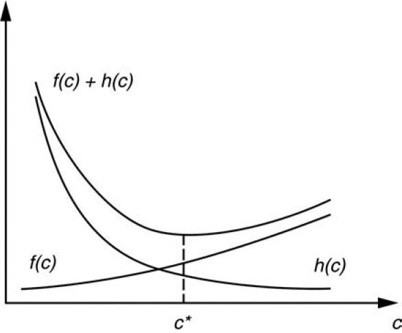
Denote the present value of the total frictional cost of capital by f(c), which is an increasing function of c. Also denote the present value of the total cost of financial distress by h(c). Then h increases as c decreases. As c falls to a certain point so that the firm is on the verge of default, h(c) rises rapidly. Assume further that both f and h are convex functions (f″(c) ≥ 0 and h″(c) ≥ 0); then there is a unique capital level c* that minimizes the present value of total frictional costs, f(c) + h(c). This can be seen from Figure 1.

Figure 1.Capital level and frictional cost

Perold (2005) and Chandra and Sherris (2005) make further assumptions in their models, including that f is a linear function of V(S), g is a linear function of d, and assets are invested risk-free. They then solve c* in a more explicit formula. To have a practical solution, however, one needs to identify major types of frictional costs and quantify each of them. So far there is little research in this area.

Note that c* is optimal for the policyholders and shareholders as a whole (or optimal for the insurance system). But if premiums are inadequate, the firm still loses money (on the present value basis), and shareholder wealth falls. Even so, reducing frictional costs is important. On one hand, if all firms charge fair premiums, the one with the lowest frictional cost has the greatest competitive advantage. On the other hand, for a given premium level on the market, the firm with the lowest frictional cost generates the highest return for its shareholders.

5. Conclusions

In this paper we thoroughly examined the impact of capital level on insurance premium and shareholder return. The solvency guarantee introduced in Merton and Perold (1993) is employed to explain the premium decrease in firms holding inadequate capital. These firms have to pay the guarantor (guaranty fund, parent firm, or policyholders) for expenses and frictional costs associated with the guarantee, which causes the net premium to fall more than the value of uncovered liabilities. It seems useful to compare the cost of various forms of guarantees. A cheaper guarantee alleviates the damage caused by inadequate capital.

In a default-free firm (where no solvency guarantee is needed) with zero frictional costs, we proved that shareholders are indifferent to changes in capital amount. Thus, the presence of solvency guarantee and that of frictional costs are the only reasons why shareholders care about the capital level. An insurance firm should strive to quantify and manage its frictional costs. To find an optimal capital level, it needs to estimate the f and h functions. The insurance industry has not paid enough attention to this issue. There are only a few papers, including Altman (1984) and Froot, Venter, and Major (2004), that provide useful estimates of frictional costs.

This paper is limited to one-period models. A multiperiod model would recognize that business continues indefinitely. A firm has value outside the balance sheet, called the franchise value. It is the value of the “name brand,” an important asset for future business. Smith, Moran, and Walczak (2003) point out that the fair insurance premium should contain a margin for the maintenance of the franchise value. Chandra and Sherris (2005) build a multiperiod model directly. The optimal capital level based on book values is likely to be different from the capital level that maximizes the market value of the firm, which includes both the book value and the franchise value.

Acknowledgments

I thank Gary Venter and Trent Vaughn for helpful suggestions. I also thank the reviewers of the journal for many constructive comments.