A Top-Down Approach to Understanding Uncertainty in Loss Ratio Estimation

1. Introduction

Many factors contribute to uncertainty in actuarial loss ratio estimates, including

• data issues (flawed data, finite sample size)

• projection issues (selection of trend, development, and on-level factors)

• judgmental adjustments for factors which cannot be directly quantified

• unforeseen external influences (law changes, coverage changes)

Most research on the topic of estimation uncertainty has focused on quantifying the effects of finite sample size [see, e.g., Kreps (1997); Van Kampen (2003); Wacek (2005)]. But this is far from the only hurdle that practicing actuaries must face–and often not the most important one.

A review of insurance industry experience over the past several years indicates that while for the most part companies do a fairly good job of estimating loss ratios, there are times when the industry as a whole gets it very wrong. This supports the argument that finite sample size is not the key driver of estimation error. Furthermore, for long-tail casualty lines of business, the error in initial loss ratio estimate is strongly correlated to the insurance market cycle and persists over a number of years. This is not surprising, since in these lines it takes a number of years for the effects of changing influences to become fully evident.

In this paper we will not attempt to identify, much less quantify, all the various “known unknowns” and “unknown unknowns” that can contribute to uncertainty in the estimation of loss ratios. Instead, we will take a top-down approach, looking at the loss ratio data itself.

2. Definitions and notation

Let’s start by establishing some notation for the different quantities to be examined; using this notation, we will define a measure of estimation error that can be studied using available data. Given a set C of companies and a set T of accident years, denote

• OLR(c, t) = original loss ratio for company c and accident year t at age 12 months,

• ULR(c, t) = ultimate loss ratio for company c and accident year t.

One measure of the discrepancy between initial loss ratio estimates and the ultimate loss ratio is the quotient

$$\mathrm{R}(c, t)=\operatorname{ULR}(c, t) / \operatorname{OLR}(c, t).$$

Others [see Wacek (2007)] have sought to understand the trajectory from OLR to ULR; the main goal of this paper is to quantify and explore the behavior of R(c, t).

2.1. Available data

Values for OLR can readily be found as the Schedule P estimate booked 12 months after the start of the accident year. While the final value of ULR may take many years to be precisely determined, we may look to the most recent Schedule P estimate of the ultimate loss ratio. Schedule P provides only 10 development years, but ISO data indicate that at this age unlimited General Liability losses are more than 93% reported (i.e., the 120-to-Ultimate development factor is less than 1.07); it seems reasonable to assume that companies’ estimates of ultimate have largely stabilized by 120 months. We consider this to be a reasonable proxy for the true ultimate loss ratio.

Of course, the latest available Schedule P loss ratio for more recent accident years reflects fewer than 10 years of development. We began this study using data available as at 12/31/2005. On this basis, our Schedule P proxy for the Accident Year 2005 ULR is the same as our proxy for the OLR–in other words, no information useful for our study can be obtained for Accident Year 2005. Similarly, the data for Accident Year 2004 would be of very little value. For purposes of this study, we selected Accident Year 2003 as the most recent accident year to include; even so, as our estimate of ULR is only 36 months old, one might question whether this cutoff is sufficient. ISO data indicate that approximately 90% of General Liability claims and 63% of the associated loss dollars are reported at 36 months, which should provide some measure of stability to companies’ ULR estimates—but certainly less than that achieved at 120 months. Because we wished to use the results of this study to project behavior for future accident years, it was desirable to include the most recent data to the extent it would be meaningful; therefore we decided to include 2003.

The loss ratio data used in this study is “as was” reserving-type data, not “as-if” trended and on-leveled prospective data. This is crucial, because we specifically want to understand how the estimation error behaves over a span of successive accident years, given changing market conditions. This is not to say that the effects of trend and on-level are being ignored: they are, in fact, incorporated in the loss ratio estimates which are the subject of our analysis, and their estimation contributes to the estimation error. As mentioned in the Introduction, most published research on estimation error focuses on the portion of estimation error which is due to finite sample size. Implicit in our current analysis of estimation error are all the factors that go into an actuary’s original estimated loss ratio: uncertainty about the form of the distribution, the trend factors, the development factors, application of professional judgment, and other known and unknown sources of uncertainty, as well as uncertainty due to finite sample size.

2.2. Remarks

For a fixed company c₀, consider the average of R(c₀, t) over a large set T of years:

$$\text { Average }\left[\mathrm{R}\left(c_{0}, t\right) \mid t \in T\right]:=\mathrm{R}\left(c_{0}\right)$$

where R(c₀) is the long-term company-specific estimation error. If the company’s loss ratio estimates are unbiased, R(c₀) should be close to 1, but it could be the case that a given company has a particular estimation bias, either upward or downward [see Kahneman and Lovello (1993)].

For a fixed accident year t₀, consider the average of R(c, t₀) over a large set C of companies:

$$\text { Average }\left[\mathrm{R}\left(c, t_{0}\right) \mid c \in C\right]:=\mathrm{R}\left(t_{0}\right)$$

where R(t₀) is the accident-year specific average estimation error across all companies. In this case, we would not necessarily expect R(t₀) to equal 1. We can think of R(t₀) as the “industry delusion factor”—the ratio of the actual loss potential faced by the insurance industry in accident year t₀ to the industry’s initial view of their loss potential. Ratios greater than 1 correspond to an initial underestimation of loss and subsequent adverse development; ratios less than 1 correspond to an initial overestimation of loss and subsequent favorable development.

The interested reader may consult Meyers (1999) for an investigation of the effects of company-specific and industry-wide uncertainty effects.

3. Data and analysis

We turned to publicly available data to see what we could learn about the behavior of the estimation error ratio R.

3.1. Description of data set and overview of analysis

For 63 of the largest casualty writers, we used Schedule P data to compile Other Liability Occurrence booked loss ratios at 12 months, and the most recent booked loss ratios as of 12/31/05, for accident years 1980–2003. No specific adjustments were made for mergers and acquisitions, though a few companies for which this was considered to be a potentially problematic issue were excluded from the sample. Not every company had data available for each year; the number of companies for a given year varied from 38 for accident year 1980 to 47 for accident years 1993—2002. It must also be noted that the definitions of data to be included in specific exhibits of the statutory blank do change over time.

For each company and accident year where OLR and ULR data were available we constructed the ratio R = ULR/OLR. As described in the remainder of Section 3, our analysis of the data indicates that

• For each accident year $t_i$ the values $\mathrm{R}\left(c, t_i\right)$ are lognormally distributed across companies $c$
• The $\mu$ and $\sigma$ parameters of these lognormal distributions are strongly linked
• The $\sigma$ parameter can be approximated by a linear function of $|\mu|$
• The $\mu$ parameter can be analyzed using time series methods

3.2. Distribution of company estimation error ratios in a fixed accident year

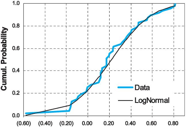
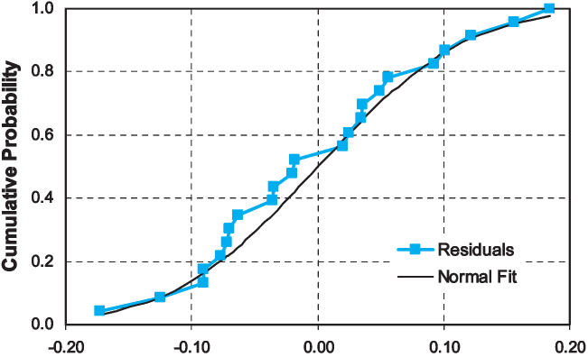
Observation of the data points in each accident year suggested that the company estimation errors might be lognormally distributed. Therefore, for each accident year $t_i$, we fitted a normal distribution to the values $\ln \left(\mathrm{R}\left(c, t_i\right)\right)$ using the method of moments, which is also the maximum likelihood fit. This is shown in Table 1.

We then applied the Kolmogorov-Smirnov test (K-S) test to compare the observed values of $\mathrm{R}\left(c, t_i\right)$ to those indicated by the lognormal approximation. For no accident year did the K-S test imply rejection of the lognormal model. A sample fit is shown in Figure 1.

Figure 1.Sample lognormal fit to $\mathrm{R}\left(c, t_i\right)$ by method of moments (AY 1999)

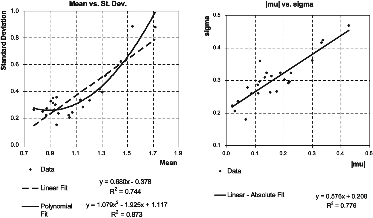
Further examination of the accident year distributions showed a strong linkage between each accident year’s mean and its standard deviation; one might also formulate this relationship as a linkage between the µ and σ parameters of the fitted lognormal distribution.

In Figure 2, each data point represents a single accident year. In the left-hand chart, year $t_i$ is represented by the point (Average[ $\left.\mathrm{R}\left(c, t_i\right) \mid c \in C\right]$, $\operatorname{Stdev}\left[\mathrm{R}\left(c, t_i\right) \mid c \in C\right]$ ) and in the right-hand chart year $t_i$ is represented by the point $\left(\mu\left(t_i\right), \sigma\left(t_i\right)\right)$. We examined various ways to express this relationship. The linear-absolute model offered a better fit than the linear model, with the simplicity of fewer parameters and greater symmetry than the polynomial fit. Therefore, we selected this linear-absolute model.

Figure 2.Mean vs. Stdev and $|\mu|$ vs. $\sigma$ for fitted lognormals

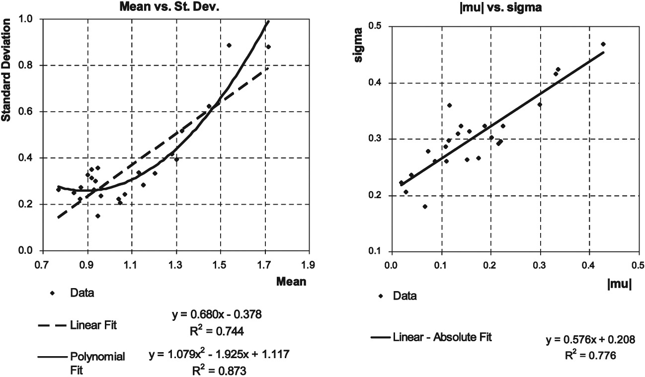
In essence this model says that the more pronounced the industry average error in a given year (whether this error is favorable or adverse), the greater the spread of the distribution across companies. The business interpretation of this could be as follows: for years when the industry as a whole does a good job of estimation, most companies will fall fairly close to the average in the accuracy of their estimates. On the other hand, for years in which the industry as a whole does a poor job of estimation, the spread of company errors is larger.

While certainly some of the spread of individual company ratios is attributable to random variation (which we assume has been largely “smoothed out” when looking at the industry average), the strength of the relationship between the µ and σ parameters of the fitted lognormal distribution suggests that the degree of spread in company values for a given accident year may be driven largely by estimation error contagion–in other words, by the level of industry delusion.

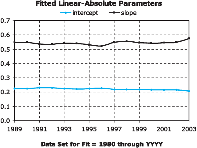
It seems reasonable to ask whether the relationship between µ and σ has remained stable over time. We tested this by fitting the slope and intercept for the linear-absolute relationship to restricted data sets, starting with accident years 1980–1989 and then successively including the next accident year to consider 1980–1990, 1980–1991, and so on. This is shown in Figure 3. We found that the linear-absolute fit remained good, with least-squares slope and intercept parameters changing only slightly over time. This consistency supports the idea that the degree of spread in company delusion around the average industry delusion in a given year may be driven more by estimation error contagion than by purely random variation.

Figure 3.Stability of fitted linear-absolute parameters relating $\sigma$ and $\mu$

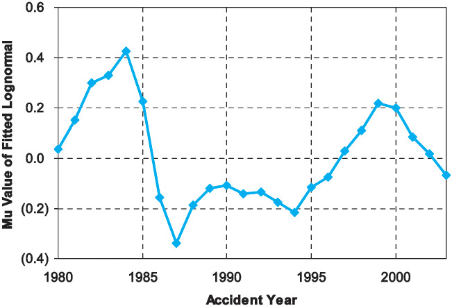
3.3. Time series analysis of the µ parameter

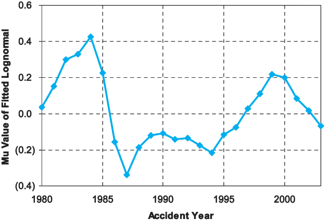
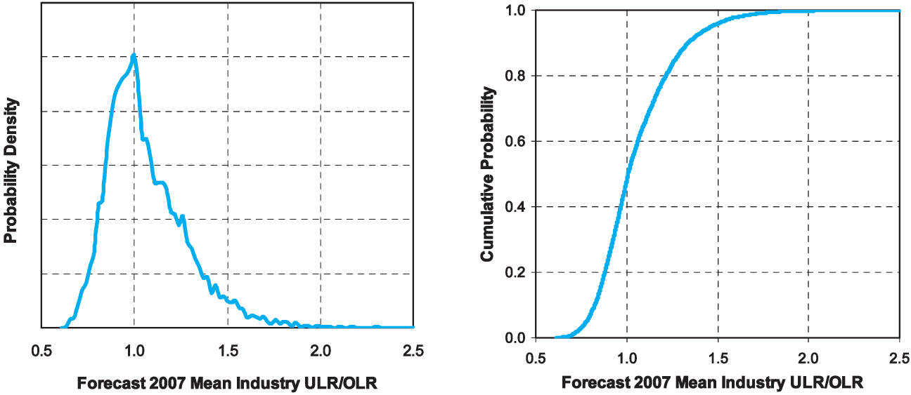
Previous sections have largely focused on the dispersion of company estimation error around the industry average estimation error for a single given accident year. Now we turn our attention to a different question: what can we say about how the value of the industry average estimation error in one accident year relates to the value of the industry average estimation error in a different accident year? In particular, we investigate the behavior of the underlying parameter, µ, across time. As can be observed from Figure 4, the behavior of the µ values indicates autocorrelation.

Figure 4.Behavior of fitted $\mu$ values over time

We examined the time series µ(t) using ARIMA methodology and identified the AR(2) model as the best fit for the data set. Using the maximum likelihood method to fit the AR(2) parameters, we obtained the following model:

$$\mu(t)=1.33 * \mu(t-1)-0.66 * \mu(t-2)+e(t).$$

This can be interpreted as saying that µ tends to “overshoot” its immediate prior value, with an offsetting effect determined by the second prior value. This is depicted in Figure 5.

Figure 5.$\mu(t)$ vs. AR(2) model

Analysis indicates that the residuals e(t) are stationary and lack autocorrelation. Furthermore, the K-S test indicates that e(t) may be approximated with a normal distribution having mean 0 and standard deviation 0.09, as shown in Figure 6.

Figure 6.Approximation of $e(t)$ by normal distribution

3.4. Applicability in practice

The AR(2) model enables the practitioner to develop a view on future years’ behavior. However, there is one significant obstacle to applicability. Our data set consists of information through 12/31/2005; consider the perspective of the actuary who, during the course of 2006, wishes to forecast the likely level of “industry delusion” for Accident Year 2007. As discussed in Section 2.1, at this point in time, the data for Accident Year 2005 is useless for this purpose, and Accident Year 2004 remains extremely green. In other words, the values of µ(t − 1) and µ(t − 2) are not yet “ripe” enough for use in projecting µ(t). If our practitioner makes the same assumption that we used for purposes of this study, namely that 2003 is the most recent accident year for which the ULR/OLR value has predictive value, in order to forecast 2007 the AR(2) formula must be applied recursively.

Alternatively, since in effect the actuary is forced to estimate accident year t using data from accident years t − 4 and t − 5, we could seek to directly fit a model that estimates µ(t) as a linear combination of µ(t − 4) and µ(t − 5). Using our 1980—2003 data set and applying the method of least squares yields

Alternate model:

$$\mu(t)=0.07 * \mu(t-4)-0.33 * \mu(t-5)+e_{\mathrm{alt}}(t) .$$

For comparison, recursive application of the AR(2) model yields

Recursive AR(2) model:

$$\left.\mu(t)=0.06 * \mu(t-4)-0.39 * \mu(t-5)+e_{\text {cumul }} t\right).$$

We can see that the coefficients are similar, as are the resulting projections, shown in Table 2.

Clearly, neither recursive application of the AR(2) model to project four steps ahead nor the alternative four-step-ahead model is as accurate as the AR(2) model applied to ripe data illustrated in Figure 5, and clearly the residuals as seen in Table 2 no longer lack autocorrelation. However, a four-step-ahead projection may still provide some insight as to the potential range of µ values in a future year. In the next section we will investigate such a projection. Given the similarity of the two models described above, we will continue with the recursive application of the AR(2) model; this offers greater theoretical simplicity and enables the development of a trajectory for µ that may provide additional insight.

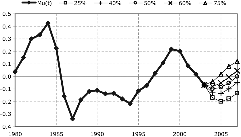
3.5. Simulation results

In order to gain additional perspective on the “probability cone” for the future trajectory of µ, we randomly generated residual values e(t) for recursive application of the AR(2) formula. The results of 10,000 Monte Carlo simulations form the probability cone depicted in Figure 7.

Figure 7.Percentiles of projection of $\mu$ for 2004-2007

In Figure 8 we graph the simulated probability density function and cumulative distribution function of the forecast industry mean error R(2007).

Figure 8.Simulated PDF and CDF for R(2007)

The median of the forecast values for R(2007) is approximately 1.0, while the mean is approximately 1.05. So, while as of 2003 the industry seems to have moved into the overestimation part of the cycle, where R = ULR/OLR is less than 1, the model suggests that by 2007 the industry could well have shifted into underestimation behavior. This can also be seen in terms of the trajectory of the projection illustrated in Figure 7; given the lognormal model, µ values greater than 0 correspond to ULR/OLR ratios greater than 1.

The 80th percentile of the simulated distribution for R(2007) is approximately 1.22, i.e., there is approximately a 20% chance that the average company’s ultimate 2007 loss ratio will be 22% higher than the initial estimate. The 95th percentile of the simulated distribution is approximately 1.47, i.e., there is approximately a 5% chance that the industry average ultimate loss ratio will be approximately 47% higher than the initial estimate. The 99th percentile is approximately 1.74, and the 99.9th percentile is approximately 2.10.

3.6. Back-testing

To investigate the reasonableness of this “four years forward” projection using recursive application of the AR(2) model, we back-tested it against our data set. Using the AR(2) parameters derived from the full 1980—2003 data set, we created simulated forecast distributions for µ in years for which we could actually calculate the value of µ from the data. We felt that the back-testing time frame of 1989—2003 could be viewed as fairly representative of a full market cycle (see Figure 4).

While we would not expect each year’s observed µ value to fall right at the center of the forecast distribution, we can compare where the observed µ values fell within the percentiles of the forecast distributions and see if the observations were distributed evenly across the distribution percentiles, or clustered inappropriately, as shown in Table 3.

We checked the percentage of µ values falling into the quintile groupings of their respective forecast distributions and found reasonably good agreement with theoretical quintiles, shown in Table 4.

As noted above, we would not expect the observed µ values to consistently fall near the center of the forecast distributions. The method cannot provide a precise point estimate of µ in future years–it’s not a crystal ball to tell us when a major shift in the industry delusion factor is on the horizon. Such shifts are generally driven by coverage changes, law changes, and so on, which are external variables that affect market behavior. However, as shown in the quintile analysis, we do find that the method is useful in projecting the likely range of possible µ values. In other words, the method does appear to provide a reasonable answer to the question “how likely are we as an industry to get it wrong—and if we do get it wrong, how wrong might we be?” As observed above, the method indicates that for the 2007 accident year, there is approximately a 20% chance that the industry average ultimate loss ratio will be at least 22% higher than the initial estimate. We believe this type of estimate is the best application of the analysis and can be used in helping companies to understand the potential for and potential magnitude of estimation error. This in turn can help companies in stress testing, making reinsurance decisions, conducting dynamic financial analysis, and applying enterprise risk management techniques.

4. Caveats

Throughout the preceding sections we have noted various limitations to this methodology. To recapitulate:

• Imperfect data. As noted earlier, definitions of data to be included in specific exhibits of the statutory blank do change over time. And, of course, companies enter and leave the business over time and/or go through mergers and acquisitions.

• ULR approximation. To the extent that reported loss ratios after several years may still be subject to additional development (either adverse or favorable) before reaching the true ultimate loss ratio, the calculated estimation error ratio may tend to be too close to 1 (i.e., µ too close to 0) and the forecast distribution may show insufficient variability.

• External “shock” influences. There have been in the past (and there surely will be in the future) external factors which influence the loss ratio estimation error. Examples include unforeseen losses such as asbestos and regulatory changes such as Sarbanes-Oxley.

• Intrinsic “component” influences. As described in the Introduction, this study was purposely created from a top-down perspective. We did not attempt to quantify or even identify all of the component influences that can contribute to uncertainty in the estimation of loss ratios. While the resulting model is not perfect, we believe that there is value in developing a model based solely on loss ratio behavior over time–one that does not explicitly rely on parameters such as loss trend, rate change, etc., which are often unreliable and/or unavailable.

The results of the back-testing shown in Table 3 suggest that overall the tail of our forecast may be somewhat conservative, in that we had no observation that fell into the highest quintile of the corresponding forecast distribution. However, with only 15 data points it is difficult to draw a firm conclusion in that regard.

5. Conclusions

The top-down approach to loss ratio estimation error we have taken in this paper–looking at the loss ratio data itself, rather than trying to quantify the individual factors that might contribute to estimation error–has two important advantages. By its nature, the method incorporates all sources of estimation error. Furthermore, unlike a bottom-up approach, this method does not require contemplation of the complicated and difficult-to-quantify relationships and codependencies among all these various contributors. Using the time series analysis and the lognormal accident year model described in this paper provides a way to help quantify the likelihood and magnitude of estimation error for current and future accident years at the industry level. This information can help companies in stress testing, making reinsurance decisions, conducting dynamic financial analysis, and applying enterprise risk management techniques.