Bias-Variance Tradeoff: A Property-Casualty Modeler’s Perspective

undefined

1. Introduction

Judging by the two popular CAS guides on GLMs, the actuarial community’s thoughts on variable selection and model validation have evolved in recent years. While the goals of modeling have always been to develop good estimators of future experience and to isolate the signal amidst the noise, our prevailing methods of model-building have evolved. Anderson et al. (2007) was initially published in the early years of actuarial modeling when predictive analytics was terra incognita in much of the industry. It rightly emphasized fundamental considerations, such as parameter-estimate standard errors, deviance (“type III”) tests, consistency testing of individual variables, and common sense.

As the actuarial community noted the developments in “statistical learning,” such subjects as overfitting, data partitioning (train/test or train/test/validate), and cross-validation began to creep more and more into our seminars and literature, and were added in the most recent general GLM “guide,” Goldburd, Khare, and Tevet (2016). Regardless of the method, however, considerable judgment and “art” are involved in building truly predictive models, as opposed to merely complex descriptive formulae. A foremost concern in this regard is avoiding overfitting.

Overfitting is a normal tendency for analytical types, and actuaries are no exception. We are naturally predisposed to examine model-trial after model-trial, sometimes straining to squeeze that last bit of intelligence from our data. Few are the modelers who, at least at some point in their career, have been immune from overfitting. While overfitting (or, in a more positive sense, optimally fitting a model) is well understood on a conceptual level, the mathematical implications of over- or underfitting may not be as well appreciated. The concept of bias-variance tradeoff can greatly enhance our understanding of the dynamics of overfitting and assist in selecting an optimal predictive model.

2. Model complexity and optimal fit

The data upon which a model is built is called the “training” data or training partition. But since we seek a model that’s truly predictive, we are less concerned about how accurately a model estimates the training partition than how the model performs on fresh data that was not used in model building. Typically, in one way or another, a portion of the available data (the “test” or “holdout” partition) is set aside, not used in model training, and used strictly to assess the model’s performance on unseen data. The model’s prediction accuracy on the test partition is an estimate of its future performance after implementation. A common measurement of the overall accuracy of a model’s prediction is the mean squared error (MSE), also known as the prediction error. If we denote the dependent variable in a dataset of n points as y, the covariates (collectively) as x, and our particular model estimator as g(x),

\[ \mathrm{MSE}=\frac{1}{n} \sum_{i}\left(y_{i}-g\left(x_{i}\right)\right)^{2} . \]

The MSEs of the training and test partitions are called the training error and test error, respectively.

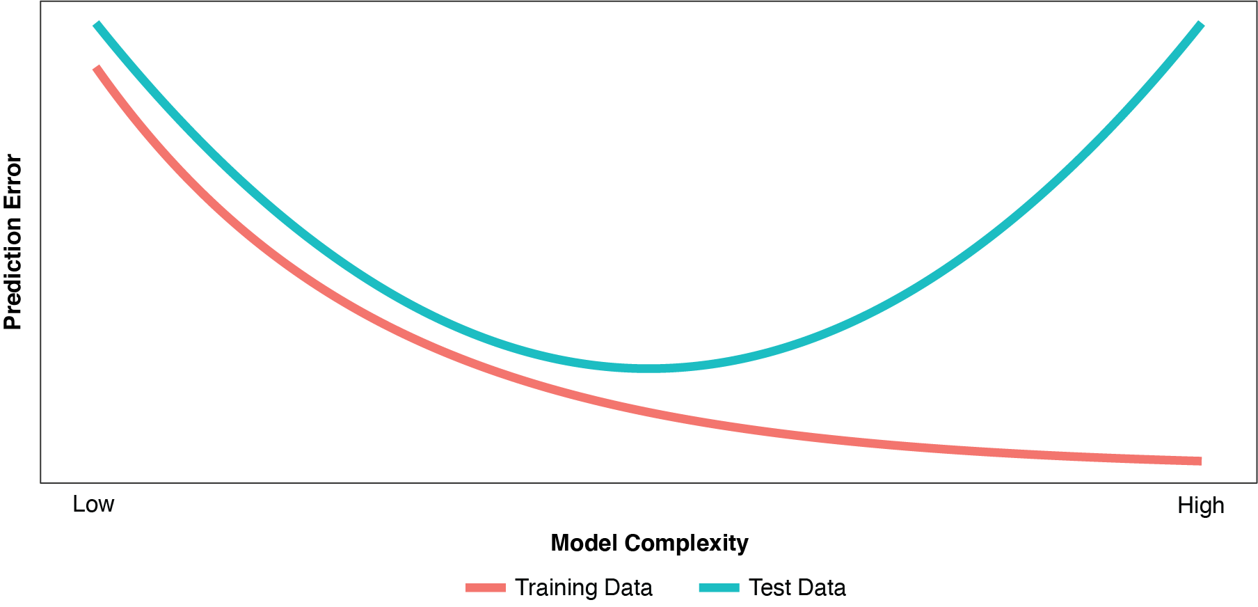
As discussed by Hastie, Tibshirani, and Friedman (2009), improvement in the training error is a major factor in our decision to add terms or nodes to our model. So, necessarily, as we dig deeper and deeper into the training data and fit the model ever more closely to the training partition, the training error continues to fall. But as depicted in Figure 1, the same is true of the test error only to a point.

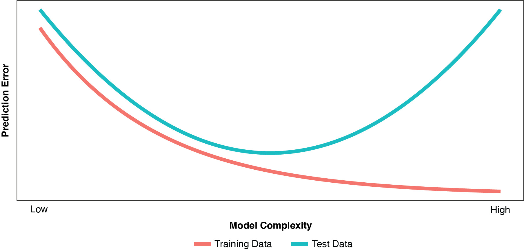
As the model becomes more complex, “overfitting” (or “overfit”) begins to occur when random variations (noise) in the training partition are misinterpreted as true relationships or “regularities” (signal). An overfit model usually has too many parameters, or variables that are defined with excess complexity. As such, while it fits the training data very well (actually, too well), the overfit model “generalizes” poorly to the test partition. The model becomes too sensitive and reactive to small fluctuations in the training data. Even with the proper number of parameters, models fit using typical techniques, such as OLS regression or un-regularized GLMs, can perform poorly on new, unseen data. As characterized by Fortmann-Roe (2012), there is a certain “sweet spot” in model complexity between underfit and overfit where the model’s performance on unseen data is optimized.

So what are we really trying to do when we model? Despite our mindfulness of the need to “separate signal from noise,” it might be easy to think that the goal of modeling is to develop an estimator for a set of observed data. It is not. Our goal as modelers is to develop an estimator for the signal underlying the observed data to the best of our ability. Our techniques, in one fashion or another, are founded upon the idea of optimizing some loss function, such as minimizing squared error or maximizing likelihood. But given a particular dataset (that is, a particular instance of all possible datasets), minimizing squared error (in the strict sense) might produce an optimal fit of the particular training partition, but not necessarily an optimal fit of the underlying signal (predictiveness).

Test error is a better estimate of predictiveness than training error, and training error is a poor estimate of test error. So even though some of the principal diagnostics used during the model-building process (parameter-estimate standard errors, deviance tests, etc.) are driven by our training partition, we need to focus on the test error in assessing predictiveness.

3. Irreducible and explainable test error

For a given point in the test partition, our observable total prediction error (the error we can see) is y − g(x). In seeking to better understand the sources of this error, it can be expressed as the sum of two sources: irreducible error and explainable error.

It helps at this point to postulate the existence of a true function, f(x)^[1], that underlies (or generates) the dependent variable in the observed data. We can express the prediction error as:

\[ y-g(x)=[y-f(x)]+[f(x)-g(x)] \]

The first component, y − f(x), is irreducible error: the difference between the observed target value and the true functional value of that point. This error is due to randomness intrinsic to the phenomenon itself. It is the natural error that is out of reach and that cannot be explained by any model.

The second component is the explainable error: the difference between the true functional value and the value estimated by our particular model for the particular point in question. This error reflects the fact that our limited training data does not fully represent all possible datasets, and it reveals the inability to produce an optimal estimator given limited data. Presumably, with infinite data and ideal estimation techniques, the explainable error could be eliminated.

This distinction between irreducible error and explainable error helps us focus on the real goal of modeling: to develop an estimator for the signal . . . the regularities or the true form . . . underlying the observable data. From this perspective there are three facts of life for modelers to accept and manage:

1. There is no such thing as infinite data. Any dataset of any size falls short of representing the totality of the true signal. We are always working with limited data, and our model needs to operate on data unseen.

2. No modeling technique (or ensemble of techniques) is perfect. There will always be a gap between the best estimator we can fashion and the true function.^[2]

3. Some error is irreducible. A portion of our prediction error not only cannot be explained by our model, but we must take steps to avoid trying to capture it in our model to avoid over-fitting.

4. Expected value in the context of bias-variance tradeoff

Before we dive into a detailed discussion of bias and variance, we first lay the groundwork for exactly what is meant by expectation in the context of bias-variance tradeoff. In practice we are given a single training sample ( \(X_1, Y_1\) ) on which to fit a model \(g\). Perhaps in an alternate reality we may have been given a different training sample ( \(X_2, Y_2\) ) on which to train \(g\). Let \(F\) represent the entire sample space, that is, the set of all possible training samples. We often denote the expectation of \(g(x)\) as \(\mathbb{E}_{\mathcal{T}}[g(x)]\) to emphasize that the expectation of \(g(x)\) is over the entire sampling space \(F\). This is a subtle, but crucial, notion for the proper appreciation of the expected value of the model estimate in understanding bias-variance tradeoff. At certain points in this discussion, this subscript is omitted for simplicity.

Ultimately, our goal is to fit a model that will perform best on unseen data. Let the space ( \(X, Y\) ) represent the holdout set on which to test the performance of our model. We assume that there is some true relationship \(f(x)=\mathbb{E}[y \mid x]\) between the target variable and covariates. It is assumed that our holdout sample ( \(X, Y\) ) is independent of our sampling space \(F\). In practice, this independence assumption often does not hold, although violation rarely results in poor-performing models.

Suppose we have some loss function, \(L(g(x), y)\), measuring the error of the model at a point \((x, y)\). We would like to know the expected error over all training sets and over the distribution of the test point \((x, y)\). That is, when we write \(\mathbb{E}[L(g(x), y)]\) the expectation is implicitly over the space of sample sets \(F\) on which the model \(g\) is fitted and over the distribution of \(y\) given \(x\). Specifically we can express the expectation as

\[ \begin{aligned} \mathbb{E}[L(g(x), y)] & =\mathbb{E}_{F}\left[\mathbb{E}_{y \mid x}[L(g(x), y) \mid x]\right] \\ & =\mathbb{E}_{y \mid x}\left[\mathbb{E}_{F}[L(g(x), y) \mid x]\right] \end{aligned} \]

With the above framework, we now define bias and variance for a model as follows:

Definition 4.1. (Bias) Let \(F=\{(X, Y)\}\) be the space of training sets for fitting model g. The bias associated with a model g at a test point (x, y) is given by

\[ \begin{aligned} \operatorname{Bias}_{f(x)}[g(x)] & =\mathbb{E}[g(x)-y \mid x]=\mathbb{E}_{\mathcal{F}}[g(x)]-\mathbb{E}[y \mid x] \\ & =\mathbb{E}_{\mathcal{F}}[g(x)]-f(x), \end{aligned} \]

where f(x) = 𝔼[y|x].

Definition 4.2. (Variance) The variance of a model g at a point x is given by

\[ \mathbb{E}\left[(g(x)-\mathbb{E}[g(x)])^{2}\right]=\mathbb{E}_{F}\left[\left(g(x)-\mathbb{E}_{F}[g(x)]\right)^{2}\right] . \]

5. The expected value of the model estimate, bias, and variance

Any particular model under consideration is but one manifestation of that model (or specifically, one manifestation of that functional form or algorithm), based on the data upon which it was trained, which as we’ve seen is one particular instance, or sample, of training data among the multitude of possible sample training datasets in our sampling space F. As such, there is a distribution of possible model estimates. Accordingly, for any particular observed point, (x, y), we can speak of the expected value of g(x), or 𝔼[g(x)]. 𝔼[g(x)], then, is the expected prediction of the model (or expected value of the “estimator”) for observed point (x, y).

Like the true prediction, f(x), the expected prediction of the model, 𝔼[g(x)], is of a speculative, or conjectural, nature; it cannot be directly measured. However, if multiple training datasets and model parameterizations could be amassed, one could approximate 𝔼[g(x)].

The explainable error, f(x) − g(x), can now be expressed as the sum of two components that are particularly relevant to our deliberation:

\[ f(x)-g(x)=(f(x)-\mathbb{E}[g(x)])+(\mathbb{E}[g(x)]-g(x)) \]

As noted in Definition 4.1, the negative of the first component, 𝔼[g(x)] − f(x), the difference between the expected prediction of the model and the value we are trying to predict (i.e., the true functional value), is the bias at point (x, y). Bias quantifies the error of the model (the algorithm, estimator or functional form, in a general sense) prediction from the true value. Consistent with Definition 4.2, the square of the negative of the second term, (g(x) − 𝔼[g(x)])², is the point’s contribution to the model’s variance.

It is important to note that the exact meaning of the term “bias” in this context is different than its classical definition. In the classical context, a statistic, or estimator, is said to be “unbiased” if it equals a population parameter. In a modeling or machine-learning context, bias refers to the difference between the expected prediction of a particular model and the point value it is intended to predict. The latter definition is presumed in this paper unless otherwise noted.

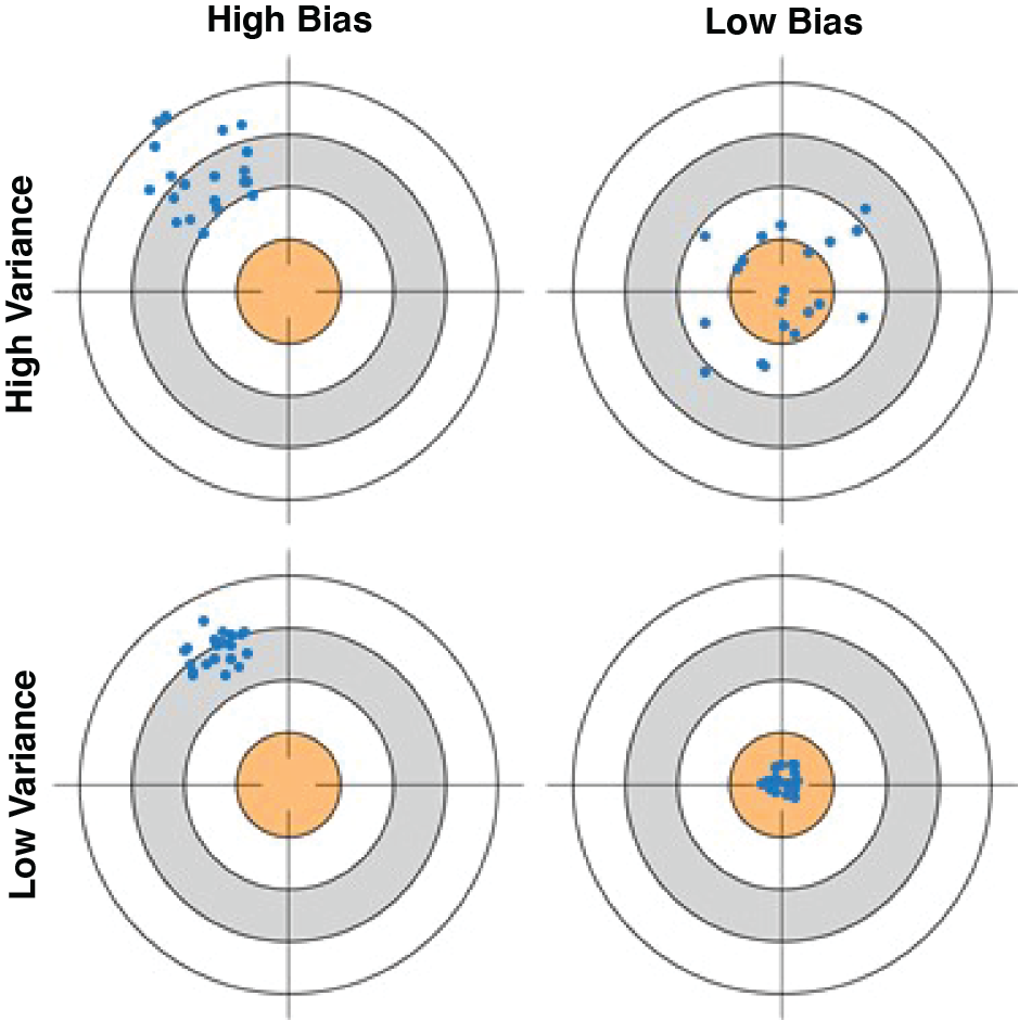
As illustrated by Hastie, Tibshirani, and Friedman (2009) and Fortmann-Roe (2012), the bullseye diagram in Figure 2 helps clarify the preceding explanations of bias and variance.

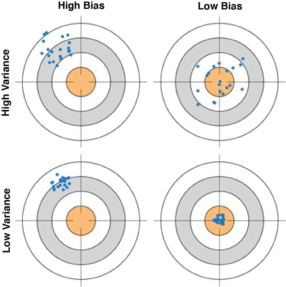
The center of the target represents perfect prediction of the true value at a test point (x, y), while the portions of the target away from its center represent predictions with error. Each point represents one manifestation of the estimator, or model, given its particular training dataset. The extent to which the various points cluster tightly represents the variance of the estimator. The extent to which the center of the point cluster approximates the center of the target represents the bias of the estimator. The top-left bullseye shows a scatter of points with both high bias and high variance: they tend to be at a distance from the true value and are broadly dispersed. The bottom-left bullseye similarly depicts a model with high bias at this value of x, but having low variance among the various possible model estimates. The bullseyes on the right illustrate low bias, where the points cluster around a center that accurately predicts the true value. The bottom-right bullseye exemplifies the modeler’s goal: an estimator algorithm that accurately predicts its true value with high reliability.

6. Decomposition of the expected squared prediction error

The preceding division of prediction error into irreducible error and explainable error, and the further division of explainable error into bias and variance components, assist us in better understanding the components of MSE on unseen (test) data. As derived in Appendix A, test prediction error can be decomposed as follows:

\[ \begin{aligned} \mathbb{E}\left[(y-g(x))^{2}\right]= & \mathbb{E}\left[(y-f(x))^{2}\right]+(\mathbb{E}[g(x)]-f(x))^{2} \\ & +\mathbb{E}\left[(g(x)-\mathbb{E}[g(x)])^{2}\right] \end{aligned} \]

The components of the above equation are recognizable, as the total test prediction error 𝔼[(y − g(x))²] is the sum of . . .

1. Irreducible squared error: 𝔼[(y − f(x))²]

2. Squared bias: (𝔼[g(x)] − f(x))²

3. and the variance of the estimator: 𝔼[(g(x) − 𝔼[g(x)])²]

As noted, while the first component, irreducible error (random noise in the observed data with respect to its true value) is beyond our control and reach, the two components of explainable error can be manipulated to achieve an optimal model.

In terms of model complexity, underfit models tend to have high bias and low variance, while overfit models tend to have low bias with high variance (low reliability in the face of new data). When starting with a moderately overfit model, the “sweet spot” of optimal predictiveness can be obtained by reducing model complexity, thereby enhancing reliability (reducing variance) at the cost of greater bias: the so-called “bias-variance tradeoff.”

It’s interesting at this point to reflect on how this concept of inviting bias into our model might be met with resistance, especially by actuaries who first learned statistics before the machine-learning era. Many statistics courses emphasized the benefits of unbiased estimators (in the classical sense of the term) to the virtual exclusion of all others, and essentially rewarded the quest for a tighter and tighter fit of the data. In essence, while this education did a good job training us to produce high-quality descriptive statistics, it may have failed to anticipate today’s greater appreciation of predictive analysis.

To illustrate these ideas we consider two simple models, a fully-parameterized model and an intercept model. For the fully-parameterized model we assume there is a single covariate labeled x with no other differentiating information considered by the model. In the case of multiple covariates, we can form the Cartesian product of all available covariates to arrive at a fully-parameterized model that considers all available information. We assume that it is possible (but not required) for each unique value of x to be sampled multiple times. The model is simply the average of the observations over each level of the covariate. For example, suppose our single covariate is whether an insured has been claims-free in the past three years. That is, x ∈{Yes, No}. In this simple case we presume to have multiple observations for both of the values “Yes” and “No.” The fitted model for “Yes” would be the average of observations for the claims-free insureds.

Example 6.1. (Fully-Parameterized Model) The fully-parameterized model is defined as g(x) = avg(y|x). That is, our prediction at x is simply the average of y over x on the training set. For each value of x we have a unique prediction.^[3]

Bias:

Clearly this estimate is unbiased at the granularity of covariate \(x\) as \(\mathbb{E}_q[g(x)]=\mathbb{E}_q[\operatorname{avg}(y \mid x)]=\) \(\operatorname{avg}\left(\mathbb{E}_q[y \mid x]\right)=\operatorname{avg}\left(\mathbb{E}_{y \mid x}[y \mid x]\right)=\mathbb{E}[y \mid x]\). The key idea is that \(\mathbb{E}_{\mathbb{F}}[y \mid x]=\mathbb{E}_{y \mid x}[y \mid x]\). That is, the expected value of the average of \(y \mid x\) over \(F\) is the expected value of \(y \mid x\).

Variance:

As the model has a separate parameter for each value of x, the resulting variance at a particular x is 𝔼[(𝔼[g(x)] − g(x))²] = 𝔼[(𝔼[y|x] − avg(y|x))²]. This is simply the variance of avg(y|x) over F. When the covariate x has many values, we would generally expect the variance to be very high. An example of such a model would be the direct use of zip code as the covariate in a territorial model. While the bias would be zero at the zip code level, the direct use of zip code would result in very high variance.

Example 6.2. (Intercept Model) The other simple model is the intercept model. That is, g(x) = y over the entire sample set.

Bias:

The bias for the intercept model is given by

\[ \mathbb{E}_{F}[g(x)]-\mathbb{E}[y \mid x]=\mathbb{E}_{F}[\bar{y}]-\mathbb{E}[y \mid x], \]

which clearly is biased except when \(\mathbb{E}_F[\bar{y}]=\mathbb{E}[y \mid x]\).

Variance:

The variance of the intercept model can be expressed as follows:

\[ \mathbb{E}\left[(\mathbb{E}[g(x)]-g(x))^{2}\right]=\mathbb{E}\left[(\mathbb{E}[y]-\bar{y})^{2}\right] \]

This is the variance of the population mean, which is relatively stable except on small data sets. Of course a constant model g(x) = c would have zero variance, but this is a less interesting model, as it has no dependence on the data.

As an illustration of these two extreme models, consider a simple situation in which f(x) = 2x, the set of x values consists of the first five positive integers, and we have three training samples, each consisting of three randomly-generated y values for each value of x.

Table 1 shows the squared bias and the sample variance for each unique value of x for each of the three samples. The sample variance, given by (g(x) – 𝔼[g(x)])², is used to illustrate the contributions to variance by each model.

As noted above, for the fully parameterized model \(\mathbb{E}[g(x)]=\mathbb{E}[y \mid x]\) which equals \(f(x)\). For the intercept model, each sample’s \(g(x)=\bar{y}\), and \(\mathbb{E}[g(x)]=\mathbb{E}_F[\bar{y}]\).. This illustrates that the fully parameterized model is unbiased, as compared to the considerable bias of the intercept model. The variance, on the other hand, is substantially lower for the simpler intercept model, reflecting the stability of the sample mean. This example illustrates extremes that may be encountered between fitting an overly simple model and an overparameterized model. As we discuss in section 9, the intercept model does not always have lower variance than a more complex “fully-parameterized” model.

7. A simulation

The following simulation (patterned after the simulation in Stansbury, n.d.) exemplifies the dynamics of bias-variance tradeoff within a family of models of various levels of complexity.

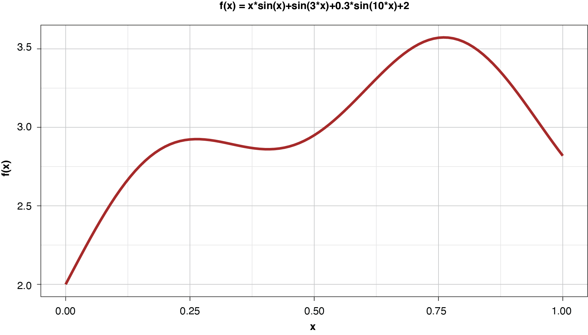
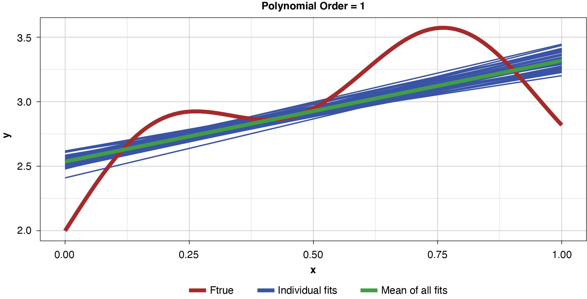
Assume that we know the “true” function that generates our observable data, as shown in Figure 3.

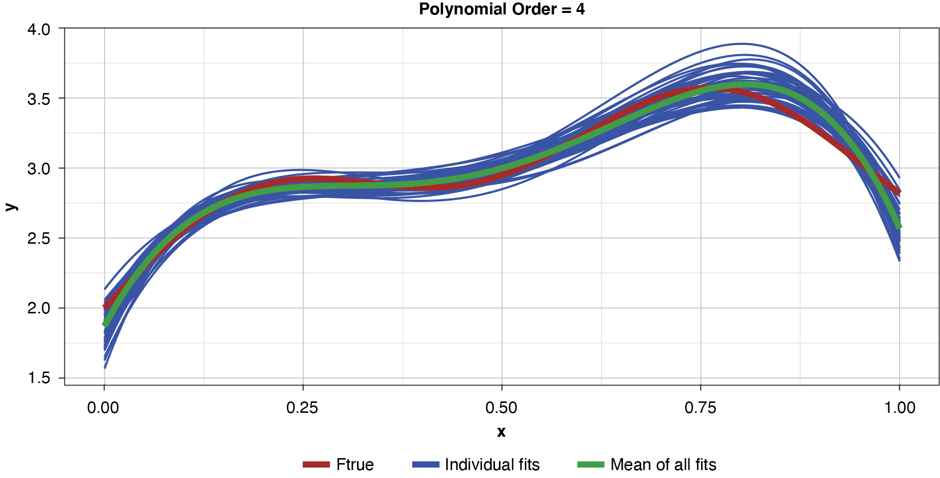
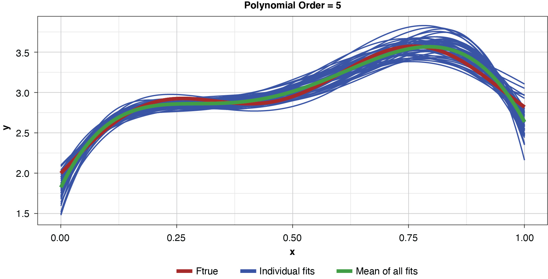
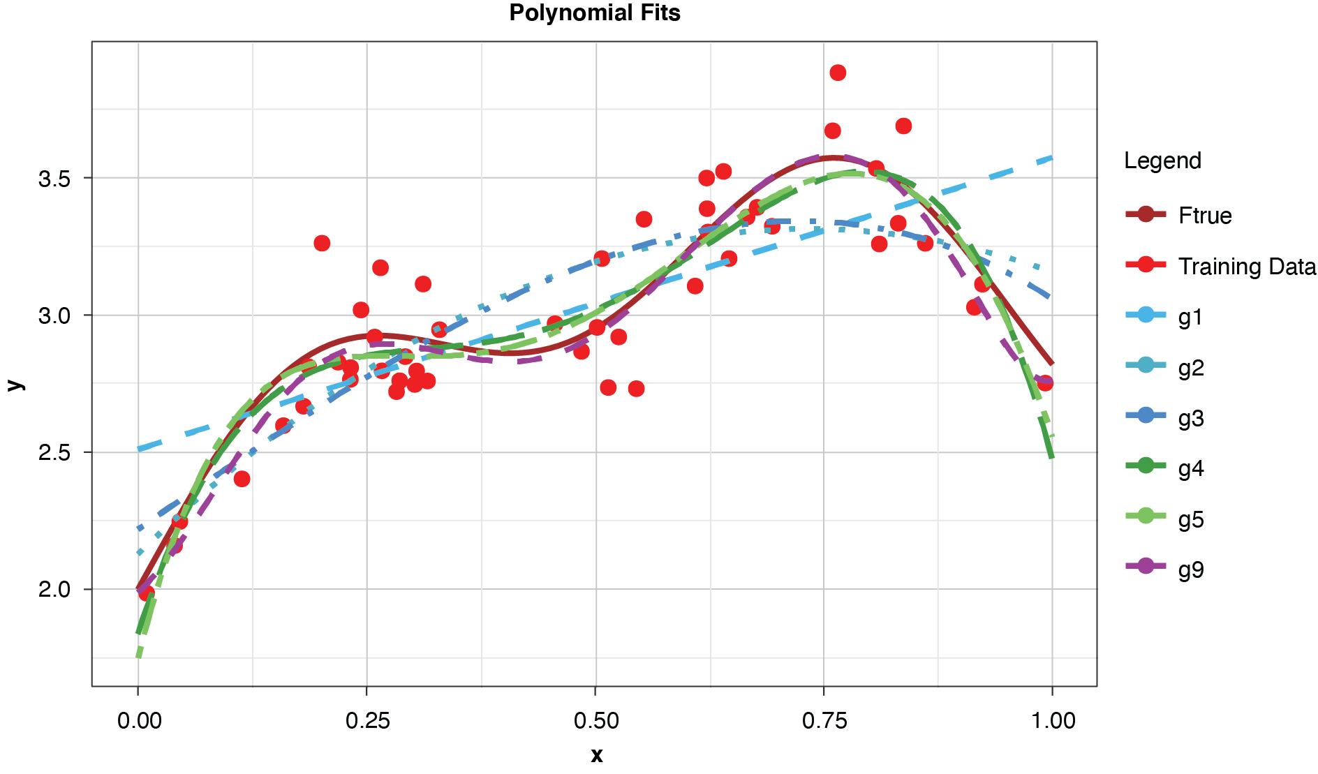
Figure 4 shows a sample of points, or training data, generated from the true function (“Ftrue”) with noise, as well as a series of polynomials of various orders (models) parameterized to the sample.

This allows us to visualize the decomposition of the prediction error into irreducible and explainable error. In terms of the preceding discussion, for any of the four models and for any particular x-value along the curve, the vertical difference between the sample value and the model-fit value is the prediction error, or y − g(x). The difference between the observed sample value and the true function is irreducible error, y − f(x), and the difference between the true functional value and the model-fit value, or f(x) − g(x), is the explainable error.

In the strict sense of the term, since this illustration involves only a single sample, we cannot measure the bias, the definition of which is based on the expected value of the estimator and the true functional value. However, if we assume for the purpose of illustration that each of the particularly-parameterized models in Figure 4 is representative of its expected value, this exhibit illustrates the relationship between bias and model complexity. The simplest model (of order of 1, or “g1”) has high bias along most of the curve, that is, it fits the true function poorly. The third-order polynomial, “g3,” begins to form itself to the true function better but still has observable bias. The higher-order polynomials, “g5” and “g9,” appear to fit the true function very well, exhibiting low bias for the preponderance of x-values. If we’re simply looking to optimize bias, we might conclude that the higher the order (the greater the complexity), the better.

But while the preceding example may demonstrate how bias varies with model complexity based on this single sample of training data, it gives us no insight into either bias in the strict sense, 𝔼[g(x)] − f(x), or the variance of the estimator, 𝔼[(g(x) − 𝔼[g(x)])²]. To accomplish that, the simulation must be expanded to involve multiple training samples (and their corresponding test samples), allowing estimation of the expected value of the estimators.

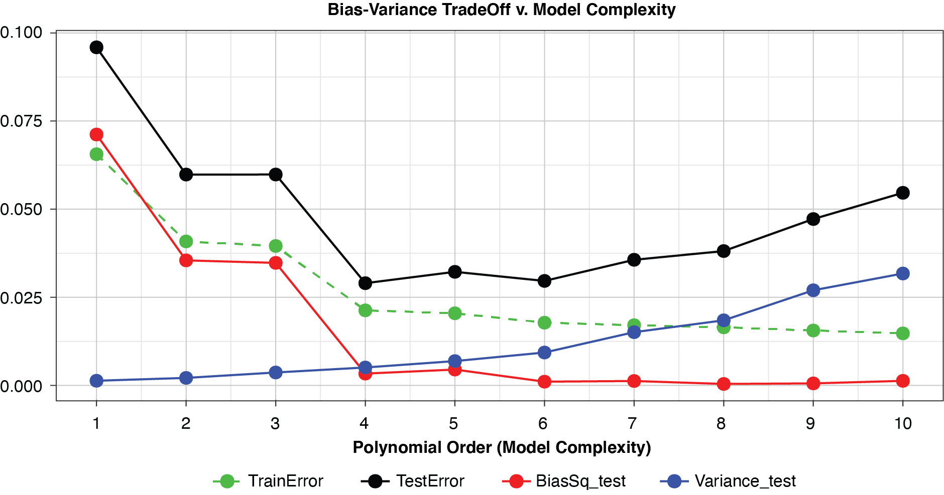
Fifty datasets of 40 points each were randomly generated and split into training and test sets of 30 and 10 points, respectively. Polynomial models of orders one through 10 were fit to each training set. In the real world we’re left to work with a single “instance” (a single sample), so this is like being able to peer into 50 “parallel universes.”

Figure 5 demonstrates the 50 simulated instances of the simplest polynomial model with 50 thin blue lines. The thicker green line in the middle of the cluster of the 50 instances is the mean of the 50 fits, providing an estimate of the expected value of the estimator, or 𝔼[g(x)]. While this simplest of models has high bias for most x values, the tight clustering of the individual fits demonstrates the model’s low variance.

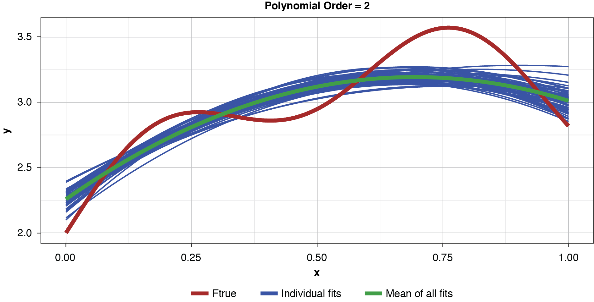
As noted previously, and as shown in Figure 6, if the model’s complexity is increased slightly (to a power of two), the bias is lessened somewhat compared to the simplest model. However, the individual fits are not as tightly clustered as in Figure 5, demonstrating the higher variance of the more complex estimator.

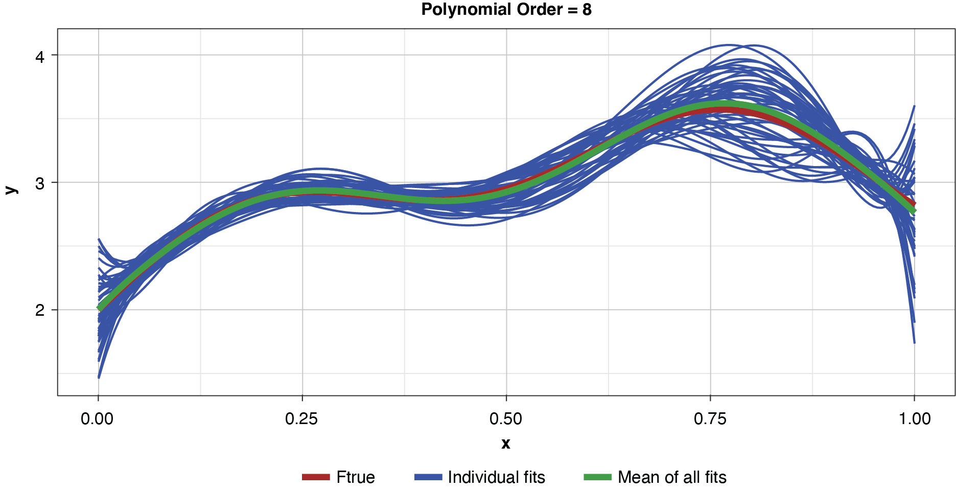
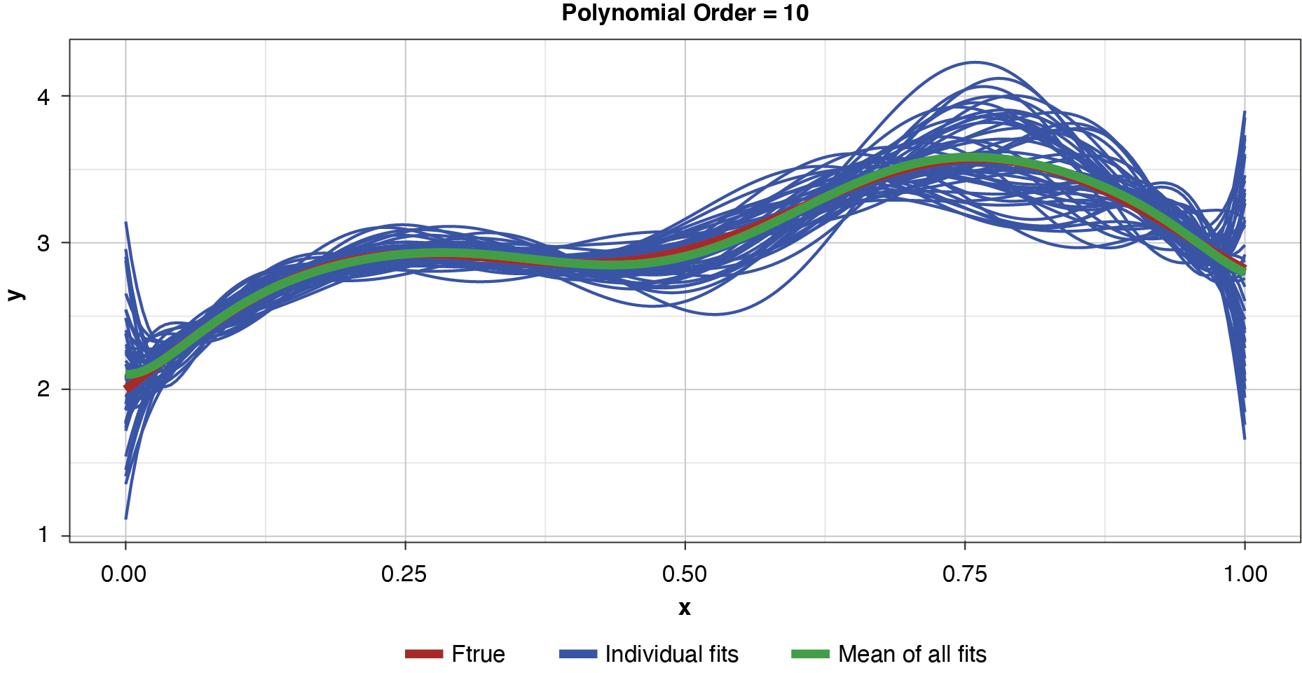
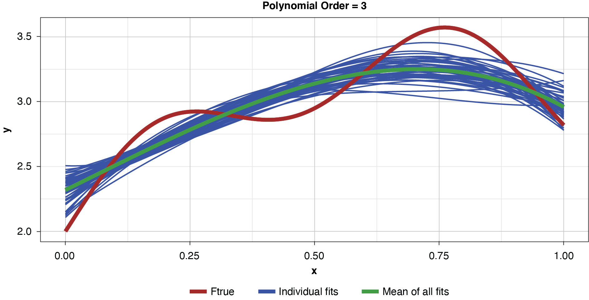
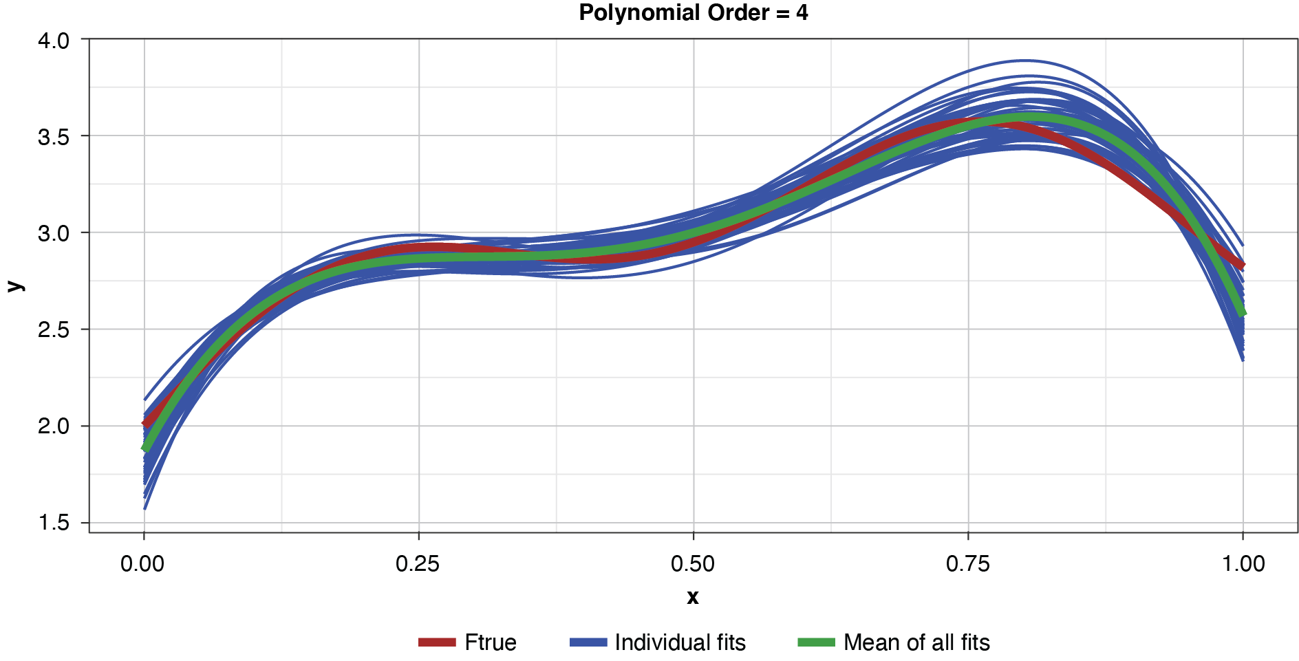
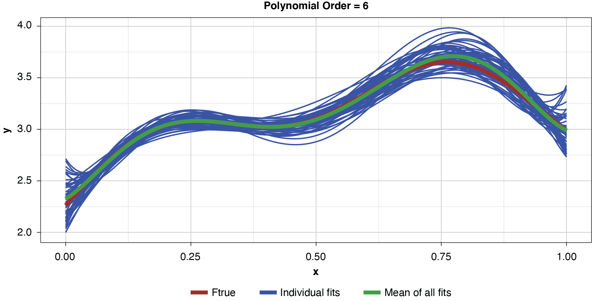
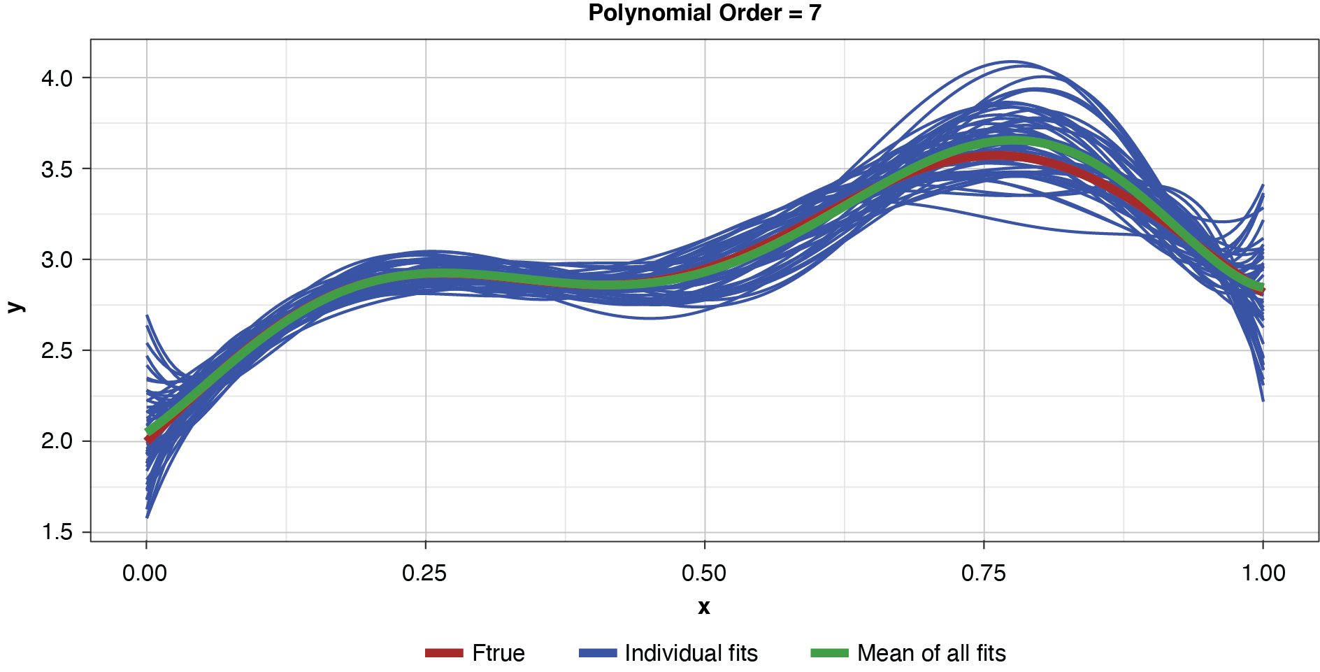
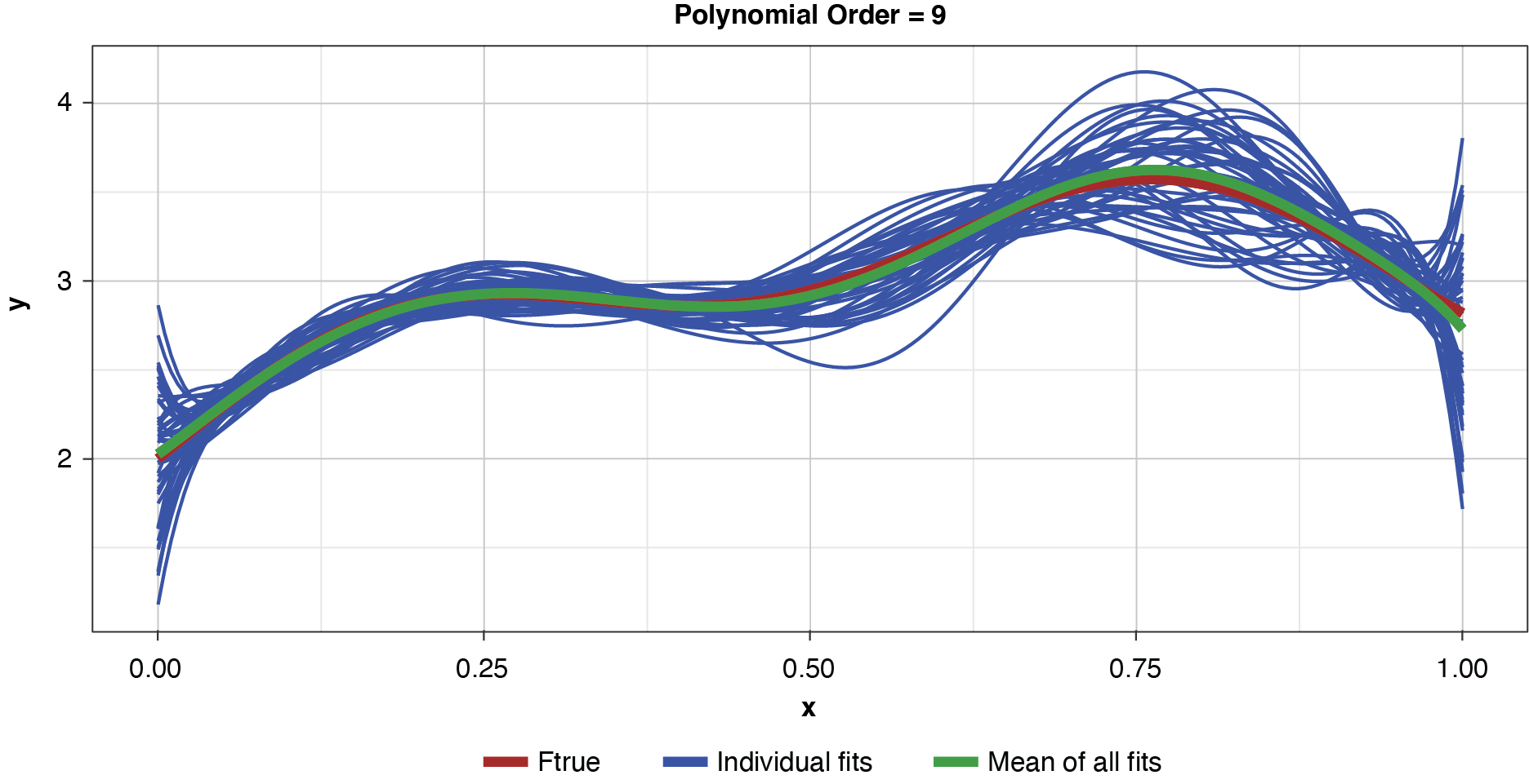
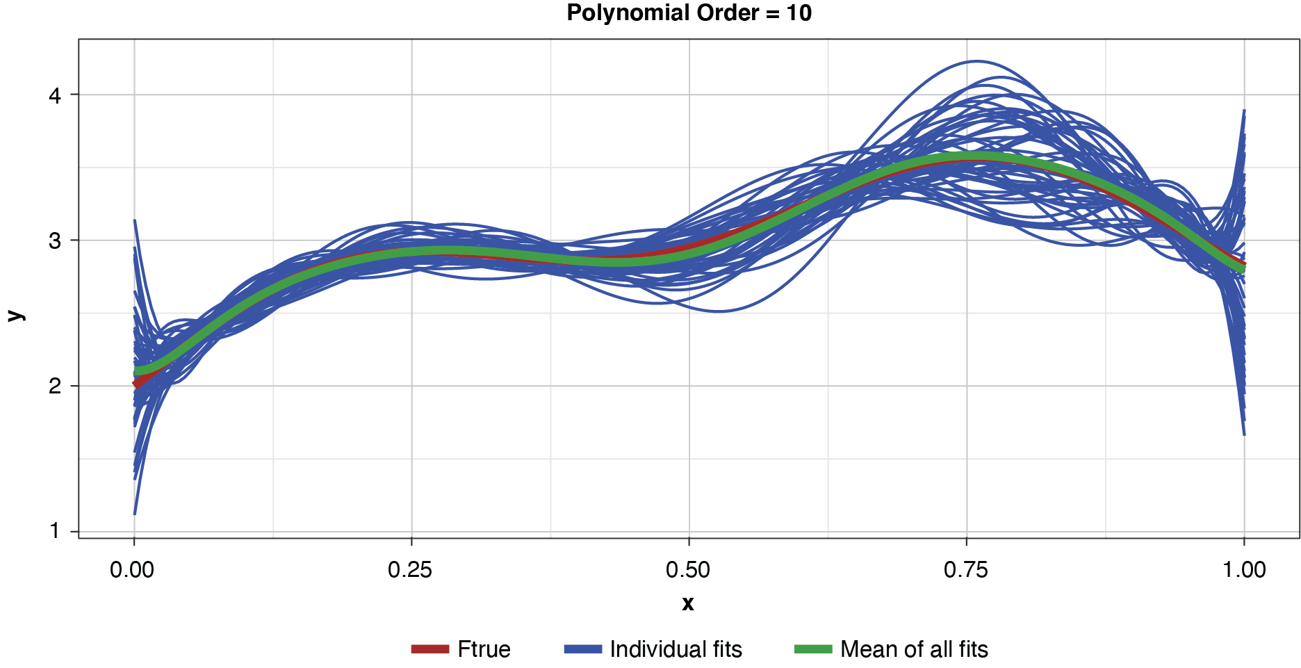
Appendix B contains all such illustrations from polynomial orders one through 10, wherein one can observe the general decrease in bias and increase in variance as model complexity increases. Figure 7 shows the most complex model.

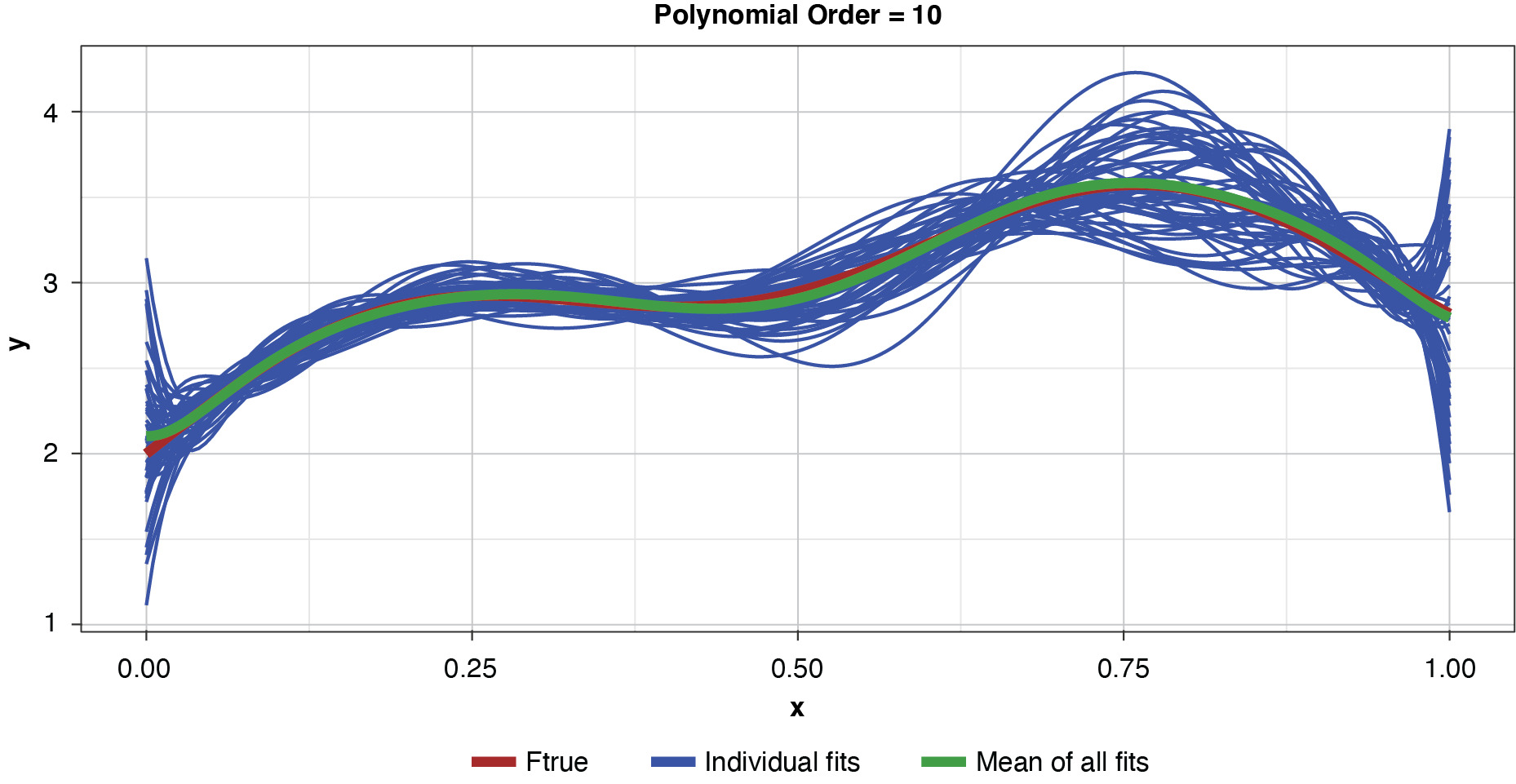
The approximated expected value of the estimator is practically coincident with the true function, indicating that bias has been almost eliminated by fitting the training data to an extreme. But the variance of the estimator is disturbingly large. This image portrays the changeability of an overfit model’s reparameterization on new data, such as a recent policy year.

Figure 8 summarizes the prediction error of both the training and test samples, as well as the squared bias and variance of the test data, for each of the models. The training prediction error decreases as model complexity increases. The test prediction error (the error on unseen data), however, decreases until the polynomial order is from four to six, then steadily increases for the most complex models, suggesting that the noise in the training data is being misinterpreted as signal. The squared bias measured on the test data decreases even to the sixth order and is minimal for the higher orders. The variance of the estimator increases progressively with model complexity. As the parameterizations are influenced increasingly by noise in the training data, the estimator becomes less and less stable. The “sweet spot” appears to be around the fourth order, where bias and variance are both modest in size. This exhibit clearly shows how, if one were working with a model of higher order, simplifying the model would result in less variability in the estimator at a price of increased bias: the bias-variance tradeoff.

8. Decomposition formula for deviance

Actuaries rarely model insurance data assuming a normal distribution. Generally a distribution from the two-parameter exponential family is relied upon.

\[ f(y \mid \theta, \phi)=\exp \left\{\frac{y \theta-b(\theta)}{\phi}+c(y, \phi)\right\} \]

We do not go into detail here, but we note that θ is a function of the linear predictor. That is, we can write θ = θ(Xβ), where X is the design matrix for the model and β are the model coefficients. We have omitted the weights from this formulation for notational simplicity. See Ohlsson and Johansson (2010) or McCullagh and Nelder (1989) for a comprehensive treatment.

For some distributions (e.g., Poisson), the dispersion parameter φ is taken to be 1 and we have a single-parameter distribution. When the dispersion parameter is applicable the general form above has two parameters. In practice we often treat φ as fixed and known with regard to estimating the coefficients of the model. How can this be? Importantly, the maximum likelihood estimate of θ is independent of φ. If one wishes to perform likelihood ratio tests or estimate the covariance of the coefficients then φ must be estimated.

As shown in Jørgensen (1992), every distribution in the exponential family is fully determined by the variance relationship linking the variance of y by function, v, of the mean. That is,

\[ \operatorname{Var}[y]=\phi v[\mu], \]

where μ = 𝔼[y|x].

Using the variance relationship we can define the deviance at a point y with parameter μ as

\[ d(y, \mu)=2 \int_{\mu}^{y} \frac{y-t}{v(t)} \mathrm{d} t. \]

This is referred to as the unscaled deviance. The scaled deviance is given by

\[ d^{*}(y, \mu)=\frac{1}{\phi} d(y, \mu) . \]

In this section we will primarily work with the unscaled deviance. If we assume φ is fixed and constant then the results in this section for the unscaled deviance also hold for the scaled deviance.

The above integral-based formula for deviance is discussed in Anderson et al. (2007). More common in the literature is the log-likelihood based definition of deviance, which is given by the difference between the saturated model and the fitted model. For our purposes the integral-based formula is more a convenient representation. In Appendix C we briefly show the equivalence between the two formulations.

The total deviance is the sum of the deviance over the data set:

\[ D(\mathbf{y}, \mu)=\sum d\left(y_{i}, \mu_{i}\right). \]

Deviance has the following properties:

1. d(y, y) = 0

2. d(y, μ) > 0 for y ≠ μ

3. The deviance increases as μ moves away from y. That is, d(y, μ₂) > d(y, μ₁) for μ₂ > μ₁ > y and μ₂ < μ₁ < y.

That is, deviance is a loss function that has larger penalties as μ moves away from y. For the normal distribution the deviance is the standard squared error:

\[ d(y, \mu)=(y-\mu)^{2}. \]

For the Poisson distribution,

\[ d(y, \mu)=\mu-y+y \log \left(\frac{y}{\mu}\right) . \]

Before proceding, we discuss the concept of minimizing the expected deviance for model g at a point x. We refer to this is the deviance-minimizing estimator.

Definition 8.1. The deviance-minimizing estimator, g̃(x) for model g at x is defined as

\[ \tilde{g}(x)=\underset{h}{\operatorname{argmin}} \mathbb{E}_{\mathcal{F}}[d(h, g(x))] . \]

That is, the deviance-minimizing estimator for model \(g\) is the value, \(h\), that minimizes the expected deviance relative to fitted values \(g(x)\) over all sampled data sets \(F\). To help motivate this definition, recall that the deviance for the normal distribution evaluated at \((h, g(x))\) is \(d(h, g(x))=(h-g(x))^2\). Suppose we wanted to find the value of \(h\) that minimizes \(\mathbb{E}_F\left[(h-g(x))^2\right]\). As this is simply the expected squared difference between h and \(g(x)\) over \(F\), the minimum value is given by the expected value of \(g(x)\). That is, \(h=\mathbb{E}_F[g(x)]\) minimizes the expected squared difference \(\mathbb{E}_F\left[(h-g(x))^2\right]\). With this example, we see that the deviance-minimizing estimator is a generalization of the property that the mean minimizes expected squared error. In Appendix C we present examples of deviance-minimizing estimators for common distributions.

Theorem 8.2. (Deviance Decomposition) As demonstrated in Appendix C, with the above definition of the deviance-minimizing estimator we can decompose the expected deviance for a model g at a test value (x, y) as

\[ \begin{aligned} \mathbb{E}[d(y, g(x))]= & \mathbb{E}[d(y, f(x)]+d(f(x), \tilde{g}(x)) \\ & +\mathbb{E}[d(\tilde{g}(x), g(x))] . \end{aligned} \]

Our inspiration for the above decomposition comes from Hansen and Heskes (2000). As compared to Hansen and Heskes (2000), we provide a further refinement of the sum of bias and irreducible error. Additionally we provide a more detailed derivation (Appendix C). The first term is the expected deviance between the observed target value and the true functional value at that point. This is analogous to irreducible error in the MSE bias-variance decomposition. The second term is the deviance of the true functional value relative to the deviance-minimizing estimator, which is a measure of bias. The third term is the expected value of the deviance between the fitted model and the deviance-minimizing estimator of the model, which is a generalization of variance.

The deviance decomposition theorem shows that the principle of bias-variance tradeoff applies, not just for MSE, but in a more generalized setting where deviance is used to evaluate goodness-of-fit.

9. Example illustrating the connection to credibility

Credibility theory, as developed by Bühlmann, introduces a biased estimator that is a blend between the raw estimate and the population average. This blend is chosen such that the estimator has the best expected performance on new data. Using a simple example below, we illustrate the connection between Bühlmann credibility and bias-variance tradeoff.

Let x be a covariate with two levels {u,d} where the target y is normally distributed with mean plus or minus a. Specifically we assume:

\[ \begin{array}{l} \mathbb{E}[y \mid x=u]=a \\ \mathbb{E}[y \mid x=d]=-a \end{array} \]

As u and d are equally likely, we assume the conditional variance is

\[ \operatorname{Var}[y \mid x]=\sigma^{2} . \]

As a consequence the unconditional variance of y is

\[ \operatorname{Var}[y]=\sigma^{2}+a^{2}. \]

This structure may look familiar. In credibility theory, σ² is the within variance and a² is the between variance.

Before moving further with the connection to credibility, let us consider the two simple models from Examples 6.1 and 6.2. For the fully-parameterized model, suppose we estimate y|x by

\[ \hat{y}(x)=g_{1}(x)=\operatorname{avg}(y \mid x)=\bar{y}_{x}, \]

that is, the average of the sample for each of the two levels of x. For the intercept model, y|x is estimated by the population average without regard to the levels of x. That is, ŷ(x) = g₂ (x) = y.

The expected MSE is calculated for each of the models. As mentioned above, we assume both levels of x are sampled equally on each training set of size n. The MSE of the fully-parameterized model is

\[ \mathbb{E}\left[\operatorname{MSE}\left(g_{1}(x)\right)\right]=\mathbb{E}\left[\left(y-g_{1}(x)\right)^{2}\right]=\sigma^{2}\left(1+\frac{2}{n}\right) . \]

Similarly for the intercept model g₂

\[ \mathbb{E}\left[\operatorname{MSE}\left(g_{2}(x)\right)\right]=\left(\sigma^{2}+a^{2}\right)\left(1+\frac{1}{n}\right) . \]

Suppose we had to choose just between these two options. Assuming the covariate has true signal we would generally assume that parameterized models would outperform an intercept model, but are there times when we would prefer the intercept model g₂ over the fully-parameterized model g₁? Focusing on the test partition, we consider the conditions under which:

\[ \begin{aligned} \mathbb{E} & {\left[\operatorname{MSE}\left(g_{2}(x)\right)\right]<\mathbb{E}\left[\operatorname{MSE}\left(g_{1}(x)\right)\right] } \\ & \Leftrightarrow\left(\sigma^{2}+a^{2}\right)\left(1+\frac{1}{n}\right)<\sigma^{2}\left(1+\frac{2}{n}\right) . \end{aligned} \]

Solving for n, we find:

\[ n<\frac{\sigma^{2}}{a^{2}}-1 . \]

We recognize the familiar Bühlmanns k = s²/a². It may seem surprising that there are any cases for which the intercept model gives superior test performance over the fully-parameterized model. For example, if σ² = 10a², then we would need at least 10 observations in order to prefer y_x to the entire sample average y.

To understand this better, we consider the traditional credibility weighting between the two estimates.

\[ \hat{y}=g_{Z}(x)=\bar{y}_{x} Z+(1-Z) \bar{y} \]

As shown in Appendix D, the expected MSE can be derived as

\[ \begin{aligned} \mathbb{E}\left[\operatorname{MSE}\left(g_{Z}\right)\right]= & \sigma^{2}+a^{2}(1-Z)^{2} \\ & +\frac{1}{n}\left(2 \sigma^{2} Z+\left(\sigma^{2}+a^{2}\right)(1-Z)^{2}\right) \end{aligned} \]

Notice that the MSE has been written in the form of the bias-variance decomposition, where

• Irreducible error = σ²

• Squared bias = a²(1 − Z)²

• Variance = \(\frac{1}{n}\)(2σ² Z + (σ² + a²) (1 − Z)²)

For the fully-parameterized model (Z = 1) the estimator is unbiased with variance 2σ²/n. For the intercept model (Z = 0) the estimator is biased with:

• Squared bias = a²

• Variance = \(\frac{1}{n}\)(σ² + a² )

Generally we prefer unbiased models over biased models, but we must also consider the contribution to the total test error by the variance. While y_x may be an unbiased model, it is possible for y_x to have higher variance than y. In fact, that is the case when a² < σ². The idea is that when there is a large amount of noise, reducing variance is more important than eliminating bias.

Naturally, the next question to ask is for what Z is the MSE minimized? Taking the derivative of 𝔼[MSE(g_Z)] and setting equal to 0, we recover a familiar Bühmann-style credibility formula.

\[ Z=\frac{n+1}{n+1+\frac{\sigma^{2}}{a^{2}}} \]

The key point is that credibility in the above context attempts to find the optimal balance between the error contributed by bias and variance. If we had an infinite sample on which to build our model, then the unbiased model would perform best out of sample. Of course, we are restricted to finite samples that are often much smaller than we would prefer.

10. Practical application

Here we briefly offer some advice on how to apply the concept of bias-variance tradeoff in practice. A complete treatment of these topics would fill volumes, among which there are already excellent resources, such as Goldburd, Khare, and Tevet (2016), James et al. (2013), and Hastie, Tibshirani, and Friedman (2009).

Given the focus of this paper, it may be surprising that it is unlikely that one would even attempt to quantify bias or variance in practice. Decomposing the expected test error into irreducible error, bias, and variance is generally not possible or even desirable. The modeler usually has little knowledge of the true population being sampled, and so it is not possible to ascertain either the expected value of the model estimate nor the true expected target value.

Our goal is to develop a model that has the best predictive power on unseen data. That is, we are concerned with minimizing the out-of-sample test error. How much the irreducible error, bias, and variance contribute to the total error is not important. Why, then, should we be concerned with the bias-variance tradeoff? Most important is that familiarity with the dynamics of bias-variance tradeoff helps build the modeler’s intuition regarding the tradeoffs associated with model complexity. This intuition is further developed by considering illustrations such as the simulation in Section 7 and the credibility example in Section 9. These examples help build a modeler’s understanding of the techniques and decisions that produce better models.

A single holdout dataset is often employed to help optimize model performance on unseen data, but there are concerns with this approach. If a modeler tests multiple models on a single holdout set, he or she may begin to overfit the holdout data. Furthermore, reserving part of the data for testing/validation reduces the amount of data available for model training, possibly resulting in fewer ascertained patterns and less confidence in the selected structure.

As an alternative to a single holdout set, cross-validation is considered to be a standard method for assessing holdout performance (Hastie, Tibshirani, and Friedman 2009). Briefly, in n-fold cross validation the training set is divided into n parts of approximately equal size. For the ith part the model is fit to the remaining n-1 parts collectively, and the resulting prediction error is computed on the ith part, which serves as a partial holdout set. The n partial-prediction-error totals are then aggregated to estimate the total test prediction error. Cross-validation has the important advantage over traditional holdout sets in that all the data is used to build and test the model. In an extension of this technique called k-times n-fold cross-validation, the cross-validation procedure is repeated k times using a different random partitioning each time. Within this framework we are simply focused on reducing the MSE as measured through cross-validation. The error contributed by noise, bias, or variance is still unknown.

When parameter estimation is discussed, it is traditionally suggested that it is preferable for estimates to have zero bias. But as noted above, bias is not the only contributor to test error. Specifically, this means bias is not necessarily something to be avoided, as long as the reduction in variance is greater than the increase in bias.

As suggested in Section 2, models with high complexity tend to overfit, and models with low complexity tend to underfit. The following considerations may assist the modeler in finding the “sweet spot” of an optimal fit:

1. Variable Selection: Adding parameters to a model generally increases model complexity, usually reducing the bias while increasing variance. In this category we include such considerations as which covariates enter the model, grouping levels of categorical variables, introducing polynomial powers, binning continuous variables, and introducing interaction terms. As described in Anderson et al. (2007), consistency testing individual covariates can assist in eliminating those with the most unstable relationships to the dependent variable. This is accomplished by examining each potential covariate’s interaction with a “time” variable, or with some other categorical variable that provides a meaningful partition of the book of business.

2. Credibility: Once a covariate is selected for inclusion in a model, it may be determined that the “raw” estimated coefficient is not optimal. Complexity can be adjusted further by choosing a balance between the coefficients fitted by least-squares regression vs. not including the covariate. Aside from traditional credibility approaches, models that implement a coefficient-blending approach are mixed-effects models as discussed in Frees, Derrig, and Meyers (2014) and elastic-net models as discussed in James et al. (2013) and Hastie, Tibshirani, and Friedman (2009). From a model-complexity perspective, reducing coefficient credibility correspondingly reduces model complexity. At first glance this may seem odd, as there are still the same number of parameters in the model (i.e., traditional degrees of freedom). But by constraining the “freedom” of the parameters, partial credibility effectively reduces complexity.

3. Bagging (or, bootstrap aggregation): Essentially, the model is built multiple times on subsamples of the dataset. A popular application of bagging is with Random Forests, in which many trees are fit and averaged. Generally, while fitting a single full tree greatly overfits the data, the variance associated with a single tree can be reduced by averaging many trees, where each tree is fit on a subset of the data (sample bagging) and a subset of covariates (feature bagging). By tuning parameters such as the number of trees, the subsampling percentage of the observations, and the subsamples of covariates, the modeler can control the balance between bias and variance. Interestingly, fitting a greater number of trees actually reduces model complexity. This may seem counterintuitive, since fitting a greater number of trees sounds like we are making the model more complicated. In fact, we are reducing the complexity as the model is more constrained. That is, with more trees being averaged, the model is less able to overfit the data.

4. Boosting: Boosting attacks the ensemble problem from a different perspective as compared to bagging. Instead of taking the average of a large number of fitted models, a large number of “weak learners” are employed serially, each one working off of the residuals of the previous iteration. While each iteration does not learn the data very strongly, the combination of the weak learners may result in a strong learner. The modeler can tune parameters such as the learning rate, the number of iterations, and the subsampling of observations and covariates. In the past few years tree-based boosting algorithms, such as xgboost, have become recognized as some of the most powerful machine-learning models.